Article

Robust Multi-Step Predictor for Electricity Markets with Real-Time Pricing

1
Centre for Data Analytics and Cognition, La Trobe University, Bundoora, VIC 3083, Australia
2
Department of Electrical Engineering and Automation, School of Electrical Engineering, Aalto University, FI-00076 Espoo, Finland
3
Department of Computer Science, Electrical and Space Engineering, Luleå Tekniska Universitet, SE-97187 Luleå, Sweden
*
Author to whom correspondence should be addressed.
Energies 2021, 14(14), 4378; https://doi.org/10.3390/en14144378
Submission received: 14 June 2021 / Revised: 12 July 2021 / Accepted: 14 July 2021 / Published: 20 July 2021
(This article belongs to the Special Issue Energy Management of Prosumer Communities)

Abstract

:
Real-time electricity pricing mechanisms are emerging as a key component of the smart grid. However, prior work has not fully addressed the challenges of multi-step prediction (Predicting multiple time steps into the future) that is accurate, robust and real-time. This paper proposes a novel Artificial Intelligence-based approach, Robust Intelligent Price Prediction in Real-time (RIPPR), that overcomes these challenges. RIPPR utilizes Variational Mode Decomposition (VMD) to transform the spot price data stream into sub-series that are optimized for robustness using the particle swarm optimization (PSO) algorithm. These sub-series are inputted to a Random Vector Functional Link neural network algorithm for real-time multi-step prediction. A mirror extension removal of VMD, including continuous and discrete spaces in the PSO, is a further novel contribution that improves the effectiveness of RIPPR. The superiority of the proposed RIPPR is demonstrated using three empirical studies of multi-step price prediction of the Australian electricity market.

1. Introduction

The global transition to renewable power generation has resulted in significant research efforts to design real-time approaches for power dispatch in power grids [1] and microgrids [2]. Real-time pricing is emerging as a solution for coordinating renewable generation with other intelligent energy resources [3], such as flexible loads [4], battery storages [5] and electric vehicles [6]. Several authors mean real-time pricing when they use the term ‘demand response’ [7]. In some works, real-time pricing refers to varying hourly prices that are determined day-ahead [8] or at the end of the day [9]. Anand and Ramasubbu [10] proposed an isolated microgrid with hourly changing real-time prices known only one hour in advance. However, a move towards real-time pricing with prices being determined one interval at a time at 5-min intervals offers powerful tools for retailers and utilities to coordinate the diverse, intelligent distributed energy resources of their customers [11]. The transformation of residential and commercial buildings into prosumers with local renewable generation is one driver for such short interval real-time pricing markets [12]. Elma et al. [13] proposed a domestic prosumer operating at five min intervals, rescheduling or curtailing loads according to forecasted local photovoltaic generation and real-time electricity prices. Mbungu et al. [14] presented a similar approach for a commercial building prosumer with photovoltaic generation and battery storage; the proposed real-time pricing scheme is built on top of a time-of-use pricing scheme. Mirakhorli and Dong [15] demonstrated that a commercial building prosumer operating under five-minute real-time pricing could achieve major electricity cost savings in comparison to time-of-use or hourly pricing. Li et al. [3] optimize a multi-energy prosumer community in a market environment with real-time prices for electricity and district heating. In some regions, electricity spot markets support real-time trading at 5 min intervals [16]. An example of such a market is the Australian spot market [17].
Alahyari and Pozo [18] presented an approach for maximizing the profits for electricity consumers participating in a demand response program. A real-time electricity price is assumed so that the price for the next hours is not known at the time of planning the demand response actions. The proposed framework is able to use a forecast of such a real-time price and is able to cope with uncertainties in the forecast. Thus, the approach presented in this paper could be directly exploited in the demand response optimization proposed by Alahyari and Pozo [18]. Moving to real-time spot prices, such as prices that change every 5 min, motivates a rethinking of energy management approaches to address a real-time timeframe. For example, weather forecasts that are crucial to consumption forecasting are usually not performed short-term to address weather disturbances. However, such a short-term forecast is provided in Thilker et al. [19]. These forecasts are advantageously used by a model-predictive controller managing indoor climate, with the goal of reducing electricity consumption while maintaining indoor comfort within specifications. Our real-time electricity price forecast is not directly comparable to the short-term weather forecast in [19], as the price remains constant for the market interval, e.g., 5 min. However, as short intervals such as 5 min become more common in real-time electricity pricing, a rethinking of energy management system research to exploit short-term generation and consumption forecast will be needed.
This article proposes a novel real-time electricity price predictor, and the Australian spot market will be used as a case study due to the availability of open data. However, our proposed approach uses generally applicable time series forecasting techniques that are not specific to spot markets, so the proposed forecasting method is adaptable to other real-time electricity markets such as those referenced above.
Time series forecasting is a mature field of study with diverse applications in academic, industrial and business contexts. It is defined as the formulation of forecasts on the basis of data in one or more time series, where time series is a collection of observations made sequentially through time [20]. A forecasting method is distinguished from a forecasting model which takes into account underlying distributions of a time series. A forecast is predicated on the current time step, forecast horizon, and evaluated using the residual forecast error. In EPF, time series forecasting methods can be grouped into three categories, statistical, machine learning and hybrid methods. Statistical methods are effective at capturing seasonality, machine learning captures non-linear behaviors of a time series such as sudden bursts or jumps, and hybrid methods break down the raw data stream into sub-components and then apply either statistical or machine learning methods on these components. Although hybrid methods exhibit high accuracy, they have only been demonstrated in theoretical settings, and this limits its value in addressing the practical challenges of balancing high accuracy with robust, real-time processing.
In this paper, we propose a new EPF method, Robust Intelligent Price Prediction in Real-time (RIPPR), to address these practical challenges. RIPPR is an ensemble technique that uses Variation Mode Decomposition (VMD) to decompose time series data streams into K sub-series, where K is chosen by particle swarm optimization (PSO) considering both forecasting accuracy and forecasting horizon. Each sub-series is modeled using a variant of Random Vector Functional Link (RVFL) neural networks, Extreme Learning Machine (ELM), for the h-step ahead point forecast. Finally, the h-step forecast for the given data stream is taken by aggregating the forecasted values for each sub-series.
The research contributions of this paper are as follows:
  • The design and development of RIPPR, a novel EPF ensemble using VMD and RVFL;
  • Optimization of the VMD module using PSO to determine optimal modes of decomposition with respect to forecast accuracy and forecast horizon;
  • Extending the VMD module to process signal edges for real-time EPF applications;
  • Evaluation of RIPPR on three benchmark datasets and one real-world dataset, using metrics of accuracy and robustness. The four datasets are from diverse energy market settings that are representative of the complexities of EPF and the robustness of the proposed method.
The rest of the paper is organized as follows; Section 2 presents related work in statistical, machine learning and hybrid methods, followed by the proposed ensemble approach for EPF. The experiments and results are presented in Section 3, and Section 4 concludes the paper.

2. Materials and Methods

2.1. Related Work

Most related work in the domain of EPF is based on statistical models that derive underlying statistical properties of the time-series data streams for the task of forecasting. Some of the examples for statistical methods are autoregressive–moving average (ARMA), autoregressive integrated moving average (ARIMA), vector autoregression (VAR), Kalman filter-based methods, Holt–Winters exponential smoothing and generalized autoregressive conditional heteroskedasticity (GARCH). Chujai et al. [21] validated the capabilities of both ARMA and ARIMA in household electric consumption forecasting. Furthermore, they evaluate using the most suitable forecasting period for the given use case. Carolina et al. [22] used the VAR forecasting model to apply to interval time series. Girish et al. [23] presented the GARCH-based one-hour-ahead price forecasting model and empirically validated it using voluminous time series generated by the electricity market of India. The main limitation of statistical methods is the inability to detect or represent the non-linear features and random changes in a time series.
In contrast, EPF based on machine learning methods such as support vector machine (SVM), artificial neural networks (ANN), fuzzy neural networks (FNN), recurrent neural networks (RNN) and randomly connected neural networks is able to capture and represent these non-linear features. Ziming et al. [24] proposed a month ahead of daily electricity price profile forecasting based on SVM; SVM is adopted to forecast the prices of peak hours in peak months. Furthermore, they validated its effectiveness using the Electric Reliability Council of Texas (ERCOT). Anand et al. [25] deployed an ANN-based PSO model to forecast future energy demand for a state of India. Both particle swarm optimization (PSO) and Genetic algorithm (GA) were developed in linear and quadratic forms, and the hybrid ANN models were applied to different series. They have empirically evaluated the results comparing with other methods such as ARIMA, linear models. From the optimization perspective, they have validated the gains of the PSO-based model over the GA-based model. Yunpeng et al. [26] proposed a model for multi-step ahead time series forecasting using long short-term memory (LSTM) RNN. Hassan et al. [27] proposed a novel model based on randomly connected RNNs for electricity load demand forecasting, and the results prove the superiority of the proposed model. Compared to statistical methods, machine learning methods capture the non-linear features and random changes to a certain extent and maintains the potential for further improvements.
A separate stream of related work has focused on hybrid models composed of one or more statistical and machine learning techniques, as single models cannot effectively extract features from a complex time series such as those in energy markets that fluctuate rapidly. Hybrid models use different data decomposition techniques to process the non-linear and non-stationary electricity-related data before applying it to the forecasting model. Wang et al. [28] proposed a novel method that uses wavelet packet transform (WPT) to decompose the time series data and particle swarm optimization based on simulated annealing (PSOSA) and Least Square Support Vector Machine (LSSVM) for wind speed forecasting and the experiments demonstrated that the WPT decomposition technique makes great improvement on the forecast accuracy. Wang et al. [29] proposed a hybrid model that consists of a two-layer decomposition technique which includes fast ensemble empirical mode decomposition (FEEMD) and Variational mode decomposition (VMD). Further, the model uses back propagation (BP) neural network optimized by the firefly algorithm (FA) as the prediction algorithm. Yang et al. [30] proposed a multi-step electricity price forecasting algorithm based on the VMD algorithm, improved multi-objective sine cosine algorithm (IMOSCA), and regularized extreme learning machine (RELM). Additionally, they ensured the model is not dependent on new information during the testing phases, thereby increasing its practical value. Kaijian et al. [31] developed a method for forecasting electricity market risk using Empirical Mode decomposition (EMD) based on the Value at Risk (VaR) model, with Exponential Weighted Moving Average (EWMA) representing individual risk factors. Separately, decomposition-based TSF methods such as a multi-objective optimization for short-term wind speed forecasting [32], an ensemble empirical mode decomposition based crude oil price forecasting [33], as well as AI-based models that use deep recurrent neural networks [34], long short term memory networks [35], and hybrid neuro-fuzzy inference [36] for energy consumption prediction were reported in the recent literature.
Despite hybrid models reporting improvements to the accuracy and prediction horizon of time series forecasts, two major limitations are inherent in the development of such models. Firstly, the use of a fixed number of components for the decomposition of the raw time-series into train and test sets, which implies the test set is required in advance in the data pre-processing stage [30]. This means the model will underperform when deployed in a real-world setting where data is acquired in a sequential manner and cannot be decomposed in advance. Additionally, the model will not be able to adapt to any changes in the data stream. Secondly, decomposition has to be conducted at the arrival of each new data point. If the time step (time between two adjacent data points) is smaller than the time taken to decompose and forecast, such models become impractical for real-world application settings.

2.2. Proposed Method

The proposed method, RIPPR, is a machine learning ensemble-based decomposition method that addresses these limitations. In brief, the proposed approach consists of five main components. The pre-processing module includes a normalization as well as an extreme outlier removal process, which is then processed by the data decomposition module. The data decomposition module decomposes a given data stream into K sub-series where the optimal parameters for the decomposition are chosen by the optimization module, including the value K. It is followed up by the Forecasting module where each sub-series is modeled with RVLF for h-step ahead point forecast, which then aggregated for each subseries in the post-processing module to produce the h-step ahead point forecast. The RIPPR process is illustrated in Figure 1. It comprises of five modules, data pre-processing, data decomposition, optimization, time series forecasting and post-processing. Each module is delineated in the following subsections.

2.2.1. Data Pre-Processing Module

The pre-processing module receives the raw time series data as input. In the context of energy markets, short-term EPF is a core capability of an energy market that drives the market’s operational activities. The short-term EPF is also called spot or day-ahead price forecasting. Here we consider raw time series data to be the spot prices that the National Electricity Market Operators use to match the supply of electricity from power stations with real-time consumption by households and businesses. All electricity in the spot market is bought and sold at the spot price.
In general, to obtain an accurate forecast, the input time series data that are used to model the forecasting model should be normalized in consideration of the new data that the model will account for in the future. Due to the high fluctuation and varying nature of the energy market, each dataset and data sample is unique, posing unique challenges for EPF. In the context of spot prices, the primary challenge is the presence of noise, including duplicated values, missing data points, and extreme outliers that will make the forecasting model weak. In RIPPR, we adopt two techniques to suppress the noise in input data streams. First, we remove the extreme values to discard extreme outliers in the input data, and second, we normalize the input data prior to feeding it to the prediction model.
Extreme values (or outliers) are data points that significantly differ from other observations, and the removal of such extreme values is considered as one of the significant steps in data pre-processing. This is because machine learning algorithms and corresponding predictions/forecasts are sensitive to the range and distribution of the input data points; therefore, outliers can mislead the training process resulting in longer training times and less accurate models. Extreme values can be of two types, (1) outliers that are introduced due to human or mechanical errors, and (2) extreme values that are caused by natural variations of a given distribution. In the context of smart grid/spot prices, the first type is rarely attested. However, a common case is the presence of extreme outliers. For instance, wholesale energy prices are influenced by a range of factors, including weather, local economic activities, international oil prices and resource availability. The availability of such factors could lead spot prices to be extremely volatile and unpredictable. Thereby, we intend to address these extreme values using extreme value analysis that use the statistical tails of the underlying distribution of the variable and find the values at the extreme end of the tails. Followed by the extreme value removal, we perform min–max normalization on the time series data to scale the time series data in the range 0 and 1. In general, the min–max normalization technique does not handle outliers and extreme values, and this is why normalization is preceded by extreme value removal.
A limitation of the min-max normalization technique is that the values used in the train-test phases can be very different from a real-world scenario, where the minimum and maximum values of a time series is not prior. It is necessary to make a realistic assumption of the min–max values based on expert knowledge of the energy market.

2.2.2. Data Decomposition Module

Time series data can exhibit a variety of patterns; therefore, splitting such time series data into several distinct components, each representing an underlying pattern category, could lead to better analysis and pattern identification. The complex characteristics of the electricity spot price market make it even harder to capture the underlying patterns in order to forecast spot prices, which makes decomposition an essential component of the proposed approach. In recent work, a number of signal decomposition algorithms that can be utilized for time series forecasting were proposed. For example, Empirical Mode Decomposition (EMD) [37], Ensemble EMD [38], Complete Ensemble EMD with adaptive noise [39], Empirical Wavelet Transform (EWT) [40] and Variational Mode Decomposition [41] are several recent signal decomposition techniques.
As stated by Wang et al. [42], Variational Mode Decomposition (VMD) is the state-of-the-art data decomposition method in signal modeling. VMD decomposes a signal into an ensemble of band-limited Intrinsic Mode Functions (IMF). It is more effective than other signal decomposition methods as it is able to generate IMF components concurrently using the ADMM optimization method [43], it can avoid the error caused during the recursive calculating and ending effect, which is a significant issue of EMD [30] and it is significantly robust to noise as well [41].
In VMD, a real-valued input signal s is decomposed into a discrete number of modes uk that have specific sparsity properties while reproducing the input. Each mode of χk is assumed to be most compact around a center pulsation ωk, which is determined along with the decomposition. Based on the original algorithm, the resulting constrained variational problem is expressed as follows.
m i n u k , ω k k | | ә t δ t + j π t   u k t e j ω k t | | 2 2 s . t .   k u k = f
where {uk}:= {u1,….,uk} and {ωk}:= {ω1,…., ωk} are shorthand notations for the set of all modes and their center frequencies, respectively, and f is the input signal. Equally, k   = k = 1 K is understood as the summation over all modes. Here, K is the total number of the decomposed modes. Since the decomposition is mainly based on the parameter K, a significant effort should be placed to select the optimal value.
To address the constrained variational problem, VMD uses an optimization methodology called ADMM [41] to select the central frequencies and intrinsic mode functions centered on those frequencies concurrently. First, minimization with respect to uk (modes) is considered, and the following is obtained for ûkn+1:
û k n + 1 ω = f ^ ω i k û i ω + λ ^ ω 2   1 + 2 α ω ω k 2
Secondly, minimization with respect to ωk (center frequencies) is considered and following is obtained for ωkn+1:
ω k n + 1 = 0 ω û k ω 2   d ω 0 û k ω 2   d ω
Here ukn+1, ωkn+1 and λn+1 are updated continuously until convergence. When the following convergence condition is met, the algorithm terminates, producing the K modes.
k | | û k n + 1 û k n | | 2 2 | | û k n | | 2 2 < ε
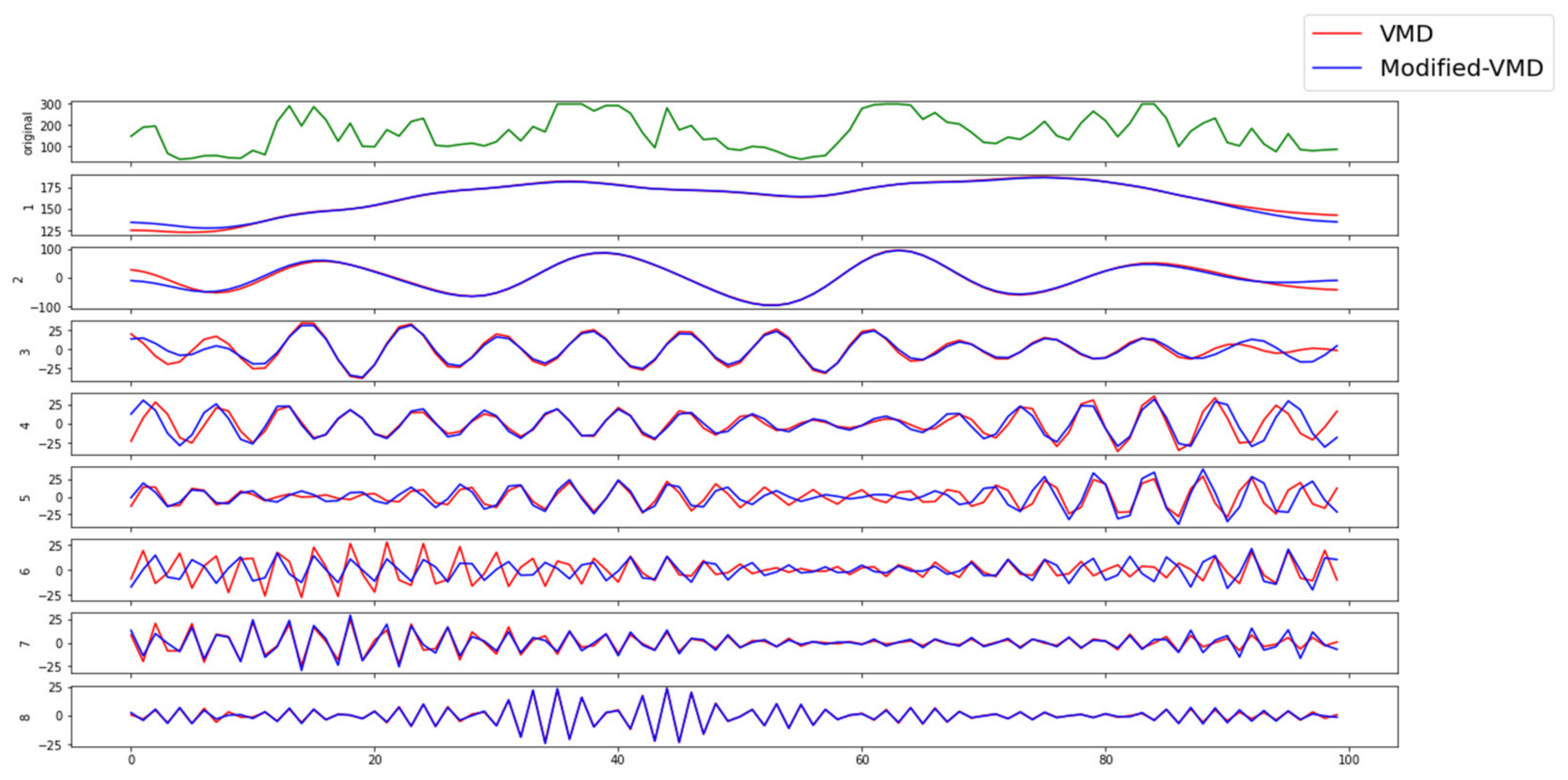
The generic VMD algorithm is effective for discrete, finite time signals; however, the boundaries of the signal are a key technical challenge due to the vanishing derivatives in the time domain boundary [41]. To address this challenge, VMD introduces a mirror extension of the signal by half its length on each side. However, this means the prediction is based on using previously seen values as future point forecasts. This is because decomposed sub-signals assume that the original signal will continue in the form of a mirror extension. Therefore, generic VMD cannot be used directly in a real-world time series forecasting setting. In RIPPR, we modified the VMD algorithm by removing this mirror extension.
In Figure 2, we compared the generic VMD algorithm and the modified version (that has the mirror extension removed) on a benchmark dataset. The results indicate that the two versions obviously differ, which will lead to different forecasting performances. However, the effectiveness of the modified-VMD algorithm is necessary for practical use.
Returning to the core capability of the VMD method, the decomposition of a signal depends on the settings of its input parameters. The VMD method consists of five parameters, namely, mode number (K-the number of modes to be recovered), balancing parameter (α-the bandwidth of extracted modes (low value of α yields higher bandwidth)), time-step of dual ascent (τ), initial omega (ω) and tolerance (ε). As experimentally proven by Dragomiretskiy and Zosso [41], ε, τ and ω has standard values across any given signal distribution. The standard values are; ε = 1 × 10⁻⁶, ω = 0, τ = 0. However, k and α depends on the signal, and this means for each new signal distribution, these two parameters needed to be adjusted. We address this in the next module using particle swarm optimization (PSO).

2.2.3. Optimization Module

The number of modes to be recovered (K) and the balancing parameter (α) determine the accuracy of the VMD decomposition. In this module, we utilize particle swarm optimization [44] (PSO) to select the most suitable values for these two values K, α, for a given forecasting horizon. We consider the prediction time for a given time-step as the objective function of the optimization technique.
PSO is a metaheuristic parallel search technique used for the optimization of continuous non-linear problems, inspired by the social behavior of bird flocking and fish schooling [45]. PSO is a global optimization algorithm for addressing optimization problems on which a point or surface in an n-dimensional space represents the best solution. In this algorithm, several cooperative agents are used, and each agent exchanges information obtained in its respective search process. Each agent, referred to as a particle, follows two rules, (1) follow the best performing particle and (2) move toward the best conditions found by the particle itself. Thereby, each particle ultimately evolves to an optimal or a near-optimal solution. PSO requires only primitive mathematical operators and is computationally inexpensive in terms of both memory requirements and speed when compared with other existing evolutionary algorithms [46].
The standard PSO (Algorithm 1) algorithm can be defined using the following equations,
v i k + 1 = ω v i k + c 1 r 1   . p b e s t , i x i k + c 2 r 2   . g b e s t x i k
Algorithm 1 Standard particle swarm optimization
Input: Objective function to be minimized (or maximized)
Parameters: swarm size, c1,c2,ω, itermax,error
Output: gbest
1: Initialize population (Number of particles = swarm size) with random position and velocity;
2: Evaluate the fitness value of each particle. Fitness evaluation is conducted by supplying the candidate solution to the objective function;
3: Update individual and global best fitness values (pbest,i and gbest). Positions are updated by comparing the newly calculated fitness values against the previous ones and replacing the pbest,i and gbest, as well as their corresponding positions, as necessary;
4: Update velocity and position of each particle in the swarm, using Equations (5) and (6);
5: Evaluate the convergence criterion. If the convergence criterion is met, terminate the process; if the iteration number equals itermax, terminate the process; otherwise, the iteration number will increase by 1 and go to step 2.
x i k + 1 = x i k + v i k + 1 α
where xi is the position of particle i; vi is the velocity of particle i; k denotes the iteration number; ω is the inertia weight; r1 and r2 are random variables uniformly distributed within (0, 1); and c1, c2 are the cognitive and social coefficient, respectively. The variable pbest,i is used to store the best position that the ith particle has found so far, and gbest is used to store the best position of all the particles. The basic PSO is influenced by a number of control parameters, namely the dimension of the problem, number of particles, step size (α), inertia weight (ω), neighborhood size, acceleration coefficients, number of iterations (itermax), and the random values that scale the contribution of the cognitive and social components. Additionally, if velocity clamping or constriction is used, the maximum velocity and constriction coefficient also influence the performance of the PSO.
A novel contribution of this module is that we have extended the basic PSO algorithm to take both continuous space (ℝ+-space) and discrete space (ℤ+-space) for optimization. In the given context, two variables exist for the optimization purpose, namely K and α. The variable α is a continuous variable, while K is a discrete variable. Therefore, we modify the basic PSO to consider both ℝ+ and ℤ+ spaces in optimization.
At the start of the algorithm, we place particles randomly such that particle position for each particle with respect to K is discrete. Then, we round off the vi(k+1) α to the nearest integer before adding it to xi (k) (Equation (6)). As such, we change Equation (6) for variable K as follows:
x i k + 1 = x i k + [ v i k + 1 α ]
where ‘[ ]’ operation represents rounding to the nearest integer.
The following section describes the fitness function that is used in the RIPPR approach. This fitness function is selected to cover both prediction accuracy as well as time taken to the prediction. The more obvious fitness function will be to use the testRMSE directly so that PSO will find an optimal (K, α) combination so that the forecasting accuracy will be higher. However, our experiments show that by doing so, it will result in a higher K value which is not desirable when considering the time taken for the prediction (K separate models will be created for each sub-series).
To overcome the aforementioned issue, we have included a penalty term to penalize having a higher K value while having good accuracy. The final fitness function is as follows:
Fitness   function   = min t e s t r m s e + β × K
where β is constant, we can control the penalizing term by adjusting the β value. From our experiments on energy price forecasting, we see that having β = 1 leads to better accuracy as well as manages to penalize having a higher K value precisely. Depending on the application, the value for K should be chosen accordingly. The calculation of the fitness function is given in Algorithm 2.
Algorithm 2 Fitness value calculation for PSO
Input: K, α, Data (X), forecasting horizon
Output: Fitness value
1: Decompose the data (X) using VMD for the given (K, α) combination;
2: Divide each sequence (sub-series) into multiple input/output patterns called samples for the given forecasting horizon;
3: Split the samples set into train and test split at a ratio of 6:4;
4: Train on the train data using the time series forecasting module for each sub-series;
5: Predict for the test data using trained models for each sub-series;
6: Aggregate the predicted values for each sub-series to obtain the final prediction for the test data;
7: Calculate the RMSE value between actual values and predicted values for the test data (testRMSE);
8: Calculate fitness value as follows: fitness   value = t e s t r m s e + β × K .
In Figure 3, we illustrate the learning process of PSO to find the optimal components for VMD. This experiment is conducted using dataset A (Table 1). We used the following parameters in the PSO algorithm, swarm_size = 10, inertia = 0.7, local_weight =2 and global weight = 2. We can see that the learning process follows the discrete–continuous search space as expected. It keeps the variable K in a discrete space while handling the alpha variable in a continuous search space. The best position for each iteration is circled in the plot with the iteration number. The spectrum of colors is used to distinguish between particles of each iteration.
Further visualization of the PSO learning process with respect to the fitness value is shown in Figure 4. On the left is the contour plot for the scattered data and on the right is the surface plot of the contour plot. The convergence of the PSO to a global optimum mainly depends on its parameters. The β × K term in the fitness function prevents looking at higher K values in the search space. Thus above-mentioned parameter configuration manages to find near-optimal components for VMD in 10–15 min of time.

2.2.4. Time Series Forecasting Module

The forecasting module generates predictions for each sub-series of the input time-series data that are decomposed by the VMD algorithm. In the context of predicting sub-series of decomposed input data, each time-step is remodeled; thus, it is not possible to use the previously trained predictive model to predict future values. Therefore, for each new time-step, the predictive model needs to be remodeled, and the re-training process should be efficient and effective to provide an accurate predictive model in a limited amount of time. This duration should ideally be less than the time between two time-steps in the time-series function.
In general, most recent approaches utilize feedforward neural networks; however, such feedforward connectionist networks are comparatively slow in training. This slow learning of feedforward neural networks continues to be a major shortcoming for EPF. The key reasons for this latency are the utilization of slow gradient-based learning algorithms and iterative tuning of all parameters of the network during the learning process. In general, randomly connected neural networks and Random Vector Functional Link (RVFL) [47] in particular are popular alternative methods for overcoming this limitation. These networks are characterized by the simplicity of RVFL’s design and training process. It makes them a very attractive alternative for solving practical machine learning problems in edge computing. Further, our recent result on the efficient FPGA implementation of RVFL [48] makes this type of network particularly suitable for the target real-time prediction scenario. Here we use a variant of RVFL known as Extreme Learning Machines (ELM) [49]. ELM is a single hidden layer feedforward neural network (SLFN) that randomly chooses input weights and analytically determines the output weights. The technical details of the ELM algorithm used for the RIPPR approach are described below.
For N arbitrary distinct input samples (xi, ti), where xi = [xi1, xi2, …, xin]T Rn and ti = [ti1, ti2, …, tim]T Rm standard SLFNs with N hidden nodes and activation function g(x) are mathematically modelled as:
i = 1 N ˜ β i g i x j = i = 1 N ˜ β i g w i . x j + b i = t j
j = 1 , , N
where wi = [wi1, wi2, …, win]T is the weight connecting the ith hidden node and the input nodes, βi = [βi1, βi2, …, βin]T is the weight connecting the ith hidden node and the output nodes, Ñ is the number of hidden layer nodes, and bi is the threshold of the ith hidden nodes. wixi denotes the inner product of wi and xi. The above N equations can be written compactly as:
H β = T ,   w h e r e H w 1 , , w N ˜ , b 1 , , b N ˜ , x 1 , , x N = g w 1 . x 1 + b 1 g w N ˜ . x 1 + b N ˜ g w 1 . x N + b 1 g w N ˜ . x N + b N ˜ N × N ˜   β = β 1 T β N ˜ T N ˜ × m   And   T = t 1 T t N ˜ T N ˜ × m
where H denotes the hidden layer’s output matrix. ELM tends to reach not only the smallest training error but also the smallest norm of output weights. According to Bartlett’s theory for feedforward neural networks reaching smaller training error, the smaller the norms of weights are, the better generalization performance of the network.
In the following formulations, 11–15, we deliberate the workings of the learning and generalization of the ELM model. Firstly, output weight optimization is solved as a minimization problem using the generalized inverse matrix of the hidden layer, followed by fine-tuning of the ELM generalization across two cases for N >> L and N > L.
The output weight can be obtained by solving the following minimization problem:
M i n i m i z e   :   | | H β T | | 2   a n d   | | β | |
where H, β and T are defined in (10). The reason to minimize the norm of the output weights | | β | | is to maximize the distance of the separating margins of the two different classes in the RVLF feature space.
The optimal solution is given by:
β = H T
where H denotes the Moore–Penrose generalized inverse matrix of the hidden layer’s output matrix, which can be calculated by the following mathematical transformation. This eliminates the lengthy training phase where network parameters will be adjusted with some hyperparameters in most learning algorithms:
H = H T H   1 H T
Input weights of the SLFN are randomly chosen, then the output weights (linking the hidden layer to the output layer) of an SLFN are analytically determined by the minimum norm least-squares solutions of a general system of linear equations. The running speed of ELM can be a thousand times faster than traditional iterative implementations of SLFNs. To further extend the generalizability of ELM, regularized extreme learning machine algorithm is introduced [50]. The original algorithm is extended by adding a regularization parameter (C) to control the generalization. This is divided into two cases as follows;
Case 1:
If the number of training data is very large, for example, it is much larger than the dimensionality of the feature space,
N >> L:
β = I C + H T H 1 H T T
Case 2:
N > L:
β = H T I C + H H T 1 T
where I is the identity matrix.

3. Experiments and Results

In this section, we evaluate RIPPR on three experiments conducted on five different datasets of EPF for the state of New South Wales (NSW), Australia. The datasets were chosen to reflect the factors of different seasons in Australia. The following section describes the experiments, their datasets and their characteristics.
The experiments were carried out on a multi-core CPU at 2.8 GHz with 16 GB memory and GPU of NVIDIA GeForce GTX 1060.

3.1. Experimental Process

First, we will consider the real-world scenario and then modify it to the experimental study (past data). Here the forecasting horizon is h (i.e., forecasts are generated for h step ahead). The full process is outlined in Algorithm 3.
Algorithm 3 Experiment procedure
Input: Data (X),h,(K,α) pair for the given h (taken from the optimization module)
Output: h step ahead forecasted value
1: Obtain the most recent 1440 data points from X(1 month period if the data rate is 30 min−1);
2: Decompose the data into K sub-series by using the data decomposition module;
3: Divide each sequence (sub-series) into multiple input/output patterns for the given forecasting horizon. Here, we will have (1440-h-input size) samples that have target values (outputs). For the experiment, the input size is kept as 24. We have (1416-h) samples. Call this train set. Last (h) samples will not have a target value. Call this test set;
4: Train on the train data using the time series forecasting module for each sub-series;
5: Predict for the test data using trained models for each sub-series;
6: Aggregate the predicted values for each sub-series to obtain the final prediction for the test data (from the h number of predicted values, the last value will give the final h-step ahead prediction for the given time frame);
7: At the arrival of a new data point, add it to the data set and remove the least recent data point from the data set and go to step (2).
For the experimental study, we start the above procedure starting from the train set and continue till the whole test set values are predicted.

3.2. Results

We report the empirical evaluation of RIPPR in terms of the following performance metrics, mean absolute error (MAE), root mean square error (RMSE), mean absolute percentage error (MAPE) and mean squared error (MSE).

3.2.1. Experiment 1

This experiment was designed as a comparative study of results for dataset A, compared between the modules of RIPPR and the available literature [29,30]. The RIPPR modules consist of ELM, VMD-ELM with a fixed K = 8 and α = 1500, VMD-PSO-ELM (Proposed RIPPR approach). The dataset is divided into train and test as follows, as the training dataset first 25 days is used. Therefore, the training dataset consists of 1200 data points. As the test dataset, the last 5 days are used. Thus, it contains 240 data points. The experiment results are shown in Table 2. The experiment compares results in three metrics, namely MAE($/MWh), RMSE($/MWh) and MAPE(%). In the experiment results, in three instances MAE and MAPE are superior to results reported in [28].
Across all instances of this experiment, RIPPR reports a better RMSE value than the literature. A key challenge in EPF is the inability to forecast outliers. From these three metrics, RMSE is the most sensitive metric to outliers. Therefore, we can confirm that our model has a more effective capability to forecast outliers than those reported in the related literature. Optimal component selection of VMD using PSO gained an advantage over the other models. A single step in this experiment represents 30 min of time.
In this comparison (Figure 5, Figure 6, Figure 7 and Figure 8), we compared five models for dataset A. The models include the Persistence model, LSTM (with two hidden layers), ELM, VMD-ELM (with a constant α-1500 and K = 8) and finally RIPPR, which uses PSO to find the optimal components for the VMD algorithm. In the first scenario (1 step ahead forecasting), it is seen that as expected, VMD-ELM outperforms the Persistence model, LSTM and the traditional ELM model by a considerable margin. The capability of RIPPR over VMD-ELM is clearly visible in the second9 scenario (Six steps ahead forecasting), where we can see that the residuals of the RIPPR are significantly lower than the VMD-ELM’s residuals. These results confirm that RIPPR can significantly outperform the VMD-ELM model. Due to the lower performance of the Persistence model and the LSTM model, we have excluded them from the later experiments.
Furthermore, to verify the significance of the accuracy improvement of the RIPPR model, the forecasting accuracy comparison with the aforementioned models is conducted using Wilcoxon signed-rank test. It is conducted under a significance level of 0.05 in one-tail-tests. The test results are presented in Table 3. It is clearly seen that there is a statistical significance (under a significance level of 0.05) for the proposed RIPPR among the compared models, including the Persistence model, LSTM model, ELM model and VMD-ELM model.

3.2.2. Experiment 2

This experiment was also designed as a comparative study for datasets B, C and D between RIPPR modules as experiment 1 and the available literature [51]. Note that here we consider the electricity load demand for the given time period. The first 3 weeks of each dataset are used to train the model, and the remaining week is used as the test set. Therefore, the training set consists of 1008 data points, and the test set consists of 336 data points. The experiment results are shown in Table 4. The experiment compares results for two metrics, namely RMSE (MW) and MAPE (%). The results clearly indicate that the RIPPR model has outperformed the available literature for all datasets. We can confirm the superiority of VMD over EMD in an EPF scenario as presented in this experiment.

3.2.3. Experiment 3

We follow the same configuration as the two previous experiments for dataset E; RIPPR vs. the available literature [52,53]. All the data were converted into hourly data similar to the literature. Thus, 1 day has 24 data points. In total, 744 data points were obtained, and 24 data points were set as test data for one step (one hour) ahead forecasting scenario. For one day (25 steps) ahead forecasting scenario, 168 data points were considered as the test data. The experimental results are shown in Table 5. The experiment compares results in 2 metrics, namely MAE($/MWh) and MSE($/MWh). In the results, the RIPPR model outperforms the compared literature by a considerable margin across all instances. The superiority of a decomposition-based hybrid model over a traditional model is also confirmed by these results. Hour-ahead forecasting is illustrated in Figure 9, and the 24-h ahead forecasting scenario is presented in Figure 10. For the 24-h ahead scenario in Figure 10, the RIPPR model has managed to capture a number of outliers in the dataset. Further, it is supported by the low MSE values across the two horizons. A single step in this experiment represents one hour of time.

4. Discussion and Conclusions

In this paper, we propose a novel Artificial Intelligence (AI) based approach for electricity price forecasting that addresses the challenges of accuracy, robustness and real-time multi-step prediction. RIPPR utilizes Variational Mode Decomposition (VMD) to transform the spot price data stream into sub-series that are optimized for robustness using particle swarm optimization (PSO). These sub-series are input to an Extreme Learning Machine (ELM) algorithm for real-time multi-step prediction. RIPPR was evaluated with six electricity price/load demand datasets from the Australian energy market. Five benchmark methods were compared with the proposed model to verify its effectiveness. Based on this robust empirical evaluation across three data streams from different market types, we can conclude that VMD based hybrid models outperform traditional single structure models in EPF, the performance of VMD depends on the mode number (k) and balancing parameter (α), and PSO optimization to find the optimal (k, α) combination improves the results significantly rather than using a static (k, α) combination. As future work, we intend to extend the proposed model to incorporate additional features such as weather, global market variables and related external events that will improve the forecast accuracy and contribute towards the AI capability for real-time monitoring of future smart grids.

Author Contributions

Conceptualization, S.K., D.D.S., S.S., R.N., A.J. and V.V.; formal analysis, D.A. and V.V.; investigation, S.K. and A.J.; methodology, S.K., D.D.S., S.S., R.N., E.O. and A.J.; resources, D.A.; software, V.V.; validation, D.D.S., S.S., R.N. and E.O.; writing—original draft, S.K., D.D.S. and S.S.; writing—review and editing, D.A., E.O., A.J. and V.V. All authors have read and agreed to the published version of the manuscript.

Funding

This research received no external funding.

Institutional Review Board Statement

Not applicable.

Informed Consent Statement

Not applicable.

Data Availability Statement

All data is publicly available from the Australian Energy Market Operator (AEMO) at https://aemo.com.au/ accessed on 4 May 2021.

Conflicts of Interest

The authors declare no conflict of interest.

Nomenclature

NomenclatureRefferd to
VMDVariational Mode Decomposition
PSOparticle swarm optimization
RVFLRandom Vector Functional Link neural network
ELMExtreme Learning Machine
EPFElectircity Price Forecasting
ARMAAuto regressive moving average
ARIMAAuto-regressive integrated moving average
VARVector auto-regression
GARCHGeneralized autoregressive conditional heteroskedasticity
ANNArtificial neural networks
SVMSupport vector machine
FNNFuzzy neural networks
RNNRecurrent neural networks
ERCOTElectric Reliability Council of Texas
LSTMLong short-term memory
WPTWavelet packet transform
PSOSAParticle swarm optimization based on simulated annealing
LSSVMLeast Square Support Vector Machine
FEEMDFast ensemble empirical mode decomposition
BPBack propagation
IMOSCAImproved multi-objective sine cosine algorithm
RELMRegularized extreme learning machine
EMDEmpirical Mode decomposition
EWMAExponential Weighted Moving Average
EWTEmpirical Wavelet Transform
SLFNSingle hidden layer feedforward neural network
NSWNew South Wales
MAEMean absolute error
RMSERoot mean square error
MAPEMean absolute percentage error

References

  1. Li, Z.; Qiu, F.; Wang, J. Data-driven real-time power dispatch for maximizing variable renewable generation. Appl. Energy 2016, 170, 304–313. [Google Scholar] [CrossRef] [Green Version]
  2. Petrollese, M.; Valverde-Isorna, L.; Cocco, D.; Cau, G.; Guerra, J. Real-time integration of optimal generation scheduling with MPC for the energy management of a renewable hydrogen-based microgrid. Appl. Energy 2016, 166, 96–106. [Google Scholar] [CrossRef]
  3. Li, Y.; Wang, C.; Li, G.; Chen, C. Optimal scheduling of integrated demand response-enabled integrated energy systems with uncertain renewable generations: A Stackelberg game approach. Energy Convers. Manag. 2021, 235, 113996. [Google Scholar] [CrossRef]
  4. Kühnlenz, F.; Nardelli, P.H.; Karhinen, S.; Svento, R. Implementing flexible demand: Real-time price vs. market integration. Energy 2018, 149, 550–565. [Google Scholar] [CrossRef] [Green Version]
  5. Lujano-Rojas, J.M.; Zubi, G.; Dufo-López, R.; Bernal-Agustín, J.L.; Catalão, J.P. Novel probabilistic optimization model for lead-acid and vanadium redox flow batteries under real-time pricing programs. Int. J. Electr. Power Energy Syst. 2018, 97, 72–84. [Google Scholar] [CrossRef]
  6. Barhagh, S.S.; Abapour, M.; Mohammadi-Ivatloo, B. Optimal scheduling of electric vehicles and photovoltaic systems in residential complexes under real-time pricing mechanism. J. Clean. Prod. 2020, 246, 119041. [Google Scholar] [CrossRef]
  7. Jiang, J.; Kou, Y.; Bie, Z.; Li, G. Optimal Real-Time Pricing of Electricity Based on Demand Response. Energy Procedia 2019, 159, 304–308. [Google Scholar] [CrossRef]
  8. Wang, F.; Ge, X.; Yang, P.; Li, K.; Mi, Z.; Siano, P.; Duić, N. Day-ahead optimal bidding and scheduling strategies for DER aggregator considering responsive uncertainty under real-time pricing. Energy 2020, 213, 118765. [Google Scholar] [CrossRef]
  9. Anees, A.; Dillon, T.; Wallis, S.; Chen, Y.-P.P. Optimization of day-ahead and real-time prices for smart home community. Int. J. Electr. Power Energy Syst. 2021, 124, 106403. [Google Scholar] [CrossRef]
  10. Anand, H.; Ramasubbu, R. A real time pricing strategy for remote micro-grid with economic emission dispatch and stochastic renewable energy sources. Renew. Energy 2018, 127, 779–789. [Google Scholar] [CrossRef]
  11. Xu, B.; Wang, J.; Guo, M.; Lu, J.; Li, G.; Han, L. A hybrid demand response mechanism based on real-time incentive and real-time pricing. Energy 2021, 231, 120940. [Google Scholar] [CrossRef]
  12. Botelho, D.; Dias, B.; de Oliveira, L.; Soares, T.; Rezende, I.; Sousa, T. Innovative business models as drivers for prosumers integration-Enablers and barriers. Renew. Sustain. Energy Rev. 2021, 144, 111057. [Google Scholar] [CrossRef]
  13. Elma, O.; Taşcıkaraoğlu, A.; Ince, A.T.; Selamogullari, U.S. Implementation of a dynamic energy management system using real time pricing and local renewable energy generation forecasts. Energy 2017, 134, 206–220. [Google Scholar] [CrossRef]
  14. Mbungu, N.T.; Bansal, R.C.; Naidoo, R.; Miranda, V.; Bipath, M. An optimal energy management system for a commercial building with renewable energy generation under real-time electricity prices. Sustain. Cities Soc. 2018, 41, 392–404. [Google Scholar] [CrossRef] [Green Version]
  15. Mirakhorli, A.; Dong, B. Market and behavior driven predictive energy management for residential buildings. Sustain. Cities Soc. 2018, 38, 723–735. [Google Scholar] [CrossRef]
  16. Finck, C.; Li, R.; Zeiler, W. Optimal control of demand flexibility under real-time pricing for heating systems in buildings: A real-life demonstration. Appl. Energy 2020, 263, 114671. [Google Scholar] [CrossRef]
  17. Forrest, S.; MacGill, I. Assessing the impact of wind generation on wholesale prices and generator dispatch in the Australian National Electricity Market. Energy Policy 2013, 59, 120–132. [Google Scholar] [CrossRef]
  18. Alahyari, A.; Pozo, D. Electric end-user consumer profit maximization: An online approach. Int. J. Electr. Power Energy Syst. 2021, 125, 106502. [Google Scholar] [CrossRef]
  19. Thilker, C.A.; Madsen, H.; Jørgensen, J.B. Advanced forecasting and disturbance modelling for model predictive control of smart energy systems. Appl. Energy 2021, 292, 116889. [Google Scholar] [CrossRef]
  20. Chatfield, C.; Routledge, B. Time-Series Forecasting, 1st ed.; CRC Press: Boca Raton, FL, USA, 2000; Available online: https://www.routledge.com/Time-Series-Forecasting/Chatfield/p/book/9781584880639 (accessed on 14 February 2021).
  21. Chujai, P.; Kerdprasop, N.; Kerdprasop, K. Time series analysis of household electric consumption with ARIMA and ARMA models. Lect. Notes Eng. Comput. Sci. 2013, 2202, 295–300. [Google Scholar]
  22. García-Ascanio, C.; Maté, C. Electric power demand forecasting using interval time series: A comparison between VAR and iMLP. Energy Policy 2010, 38, 715–725. [Google Scholar] [CrossRef]
  23. Girish, G. Spot electricity price forecasting in Indian electricity market using autoregressive-GARCH models. Energy Strat. Rev. 2016, 11–12, 52–57. [Google Scholar] [CrossRef]
  24. Ma, Z.; Zhong, H.; Xie, L.; Xia, Q.; Kang, C. Month ahead average daily electricity price profile forecasting based on a hybrid nonlinear regression and SVM model: An ERCOT case study. J. Mod. Power Syst. Clean Energy 2018, 6, 281–291. [Google Scholar] [CrossRef]
  25. Anand, A.; Suganthi, L. Forecasting of Electricity Demand by Hybrid ANN-PSO Models. In Deep Learning and Neural Networks; IGI Global: Hershey, PA, USA, 2020; pp. 865–882. Available online: https://www.igi-global.com/gateway/chapter/237910 (accessed on 3 March 2021).
  26. Yunpeng, L.; Di, H.; Junpeng, B.; Yong, Q. Multi-step Ahead Time Series Forecasting for Different Data Patterns Based on LSTM Recurrent Neural Network. In Proceedings of the 2017 14th Web Information Systems and Applications Conference (WISA), Liuzhou, China, 11–12 November 2017; pp. 305–310. [Google Scholar]
  27. Hassan, S.; Khosravi, A.; Jaafar, J.; Khanesar, M.A. A systematic design of interval type-2 fuzzy logic system using extreme learning machine for electricity load demand forecasting. Int. J. Electr. Power Energy Syst. 2016, 82, 1–10. [Google Scholar] [CrossRef]
  28. Wang, J.-Z.; Wang, Y.; Jiang, P. The study and application of a novel hybrid forecasting model–A case study of wind speed forecasting in China. Appl. Energy 2015, 143, 472–488. [Google Scholar] [CrossRef]
  29. Wang, D.; Luo, H.; Grunder, O.; Lin, Y.; Guo, H. Multi-step ahead electricity price forecasting using a hybrid model based on two-layer decomposition technique and BP neural network optimized by firefly algorithm. Appl. Energy 2017, 190, 390–407. [Google Scholar] [CrossRef]
  30. Yang, W.; Wang, J.; Niu, T.; Du, P. A novel system for multi-step electricity price forecasting for electricity market management. Appl. Soft Comput. 2020, 88, 106029. [Google Scholar] [CrossRef]
  31. He, K.; Wang, H.; Du, J.; Zou, Y. Forecasting Electricity Market Risk Using Empirical Mode Decomposition (EMD)—Based Multiscale Methodology. Energies 2016, 9, 931. [Google Scholar] [CrossRef] [Green Version]
  32. Liu, Z.; Jiang, P.; Zhang, L.; Niu, X. A combined forecasting model for time series: Application to short-term wind speed forecasting. Appl. Energy 2020, 259, 114137. [Google Scholar] [CrossRef]
  33. Abdollahi, H. A novel hybrid model for forecasting crude oil price based on time series decomposition. Appl. Energy 2020, 267, 115035. [Google Scholar] [CrossRef]
  34. Chitalia, G.; Pipattanasomporn, M.; Garg, V.; Rahman, S. Robust short-term electrical load forecasting framework for commercial buildings using deep recurrent neural networks. Appl. Energy 2020, 278, 115410. [Google Scholar] [CrossRef]
  35. Somu, N.; MR, G.R.; Ramamritham, K. A hybrid model for building energy consumption forecasting using long short term memory networks. Appl. Energy 2020, 261, 114131. [Google Scholar] [CrossRef]
  36. Jallal, M.A.; González-Vidal, A.; Skarmeta, A.F.; Chabaa, S.; Zeroual, A. A hybrid neuro-fuzzy inference system-based algorithm for time series forecasting applied to energy consumption prediction. Appl. Energy 2020, 268, 114977. [Google Scholar] [CrossRef]
  37. Huang, N.E.; Shen, Z.; Long, S.R.; Wu, M.C.; Shih, H.H.; Zheng, Q.; Yen, N.-C.; Tung, C.C.; Liu, H.H. The empirical mode decomposition and the Hilbert spectrum for nonlinear and non-stationary time series analysis. Proc. R. Soc. A Math. Phys. Eng. Sci. 1998, 454, 903–995. [Google Scholar] [CrossRef]
  38. Wu, Z.H.; Huang, N.E. Ensemble empirical mode decomposition: A noise-assistant data analysis method. Adv. Adapt. Data Anal. 2009, 1, 1–41. [Google Scholar] [CrossRef]
  39. Torres, M.E.; Colominas, M.A.; Schlotthauer, G.; Flandrin, P. A complete ensemble empirical mode decomposition with adaptive noise. In Proceedings of the 2011 IEEE International Conference on Acoustics, Speech and Signal Processing (ICASSP), Prague, Czech Republic, 22–27 May 2011; pp. 4144–4147. [Google Scholar] [CrossRef]
  40. Gilles, J. Empirical Wavelet Transform. IEEE Trans. Signal. Process. 2013, 61, 3999–4010. [Google Scholar] [CrossRef]
  41. Dragomiretskiy, K.; Zosso, D. Variational Mode Decomposition. IEEE Trans. Signal. Process. 2014, 62, 531–544. [Google Scholar] [CrossRef]
  42. Wang, Y.; Markert, R.; Xiang, J.; Zheng, W. Research on variational mode decomposition and its application in detecting rub-impact fault of the rotor system. Mech. Syst. Signal. Process. 2015, 60–61, 243–251. [Google Scholar] [CrossRef]
  43. Aneesh, C.; Kumar, S.; Hisham, P.; Soman, K. Performance Comparison of Variational Mode Decomposition over Empirical Wavelet Transform for the Classification of Power Quality Disturbances Using Support Vector Machine. Procedia Comput. Sci. 2015, 46, 372–380. [Google Scholar] [CrossRef] [Green Version]
  44. Hossain, M.A.; Chakrabortty, R.K.; Ryan, M.; Pota, H.R. Energy Management of Community Microgrids Considering Uncertainty using Particle Swarm Optimisation. Preprints 2020. [Google Scholar] [CrossRef]
  45. Kennedy, J.; Eberhart, R. Particle swarm optimization. In Proceedings of the ICNN’95 International Conference on Neural Networks, Perth, Australia, 27 November–1 December 1995; Volume 4, pp. 1942–1948. [Google Scholar]
  46. Prakash, K.N.; Sydulu, M. Particle Swarm Optimization Based Capacitor Placement on Radial Distribution Systems. In Proceedings of the 2007 IEEE Power Engineering Society General Meeting, Tampa, FL, USA, 24–28 June 2007; pp. 1–5. [Google Scholar]
  47. Igelnik, B.; Pao, Y.-H. Stochastic choice of basis functions in adaptive function approximation and the functional-link net. IEEE Trans. Neural Netw. 1995, 6, 1320–1329. [Google Scholar] [CrossRef] [Green Version]
  48. Kleyko, D.; Kheffache, M.; Frady, E.P.; Wiklund, U.; Osipov, E. Density Encoding Enables Resource-Efficient Randomly Connected Neural Networks. IEEE Trans. Neural Networks Learn. Syst. 2020, 1–7. [Google Scholar] [CrossRef]
  49. Huang, G.B.; Zhu, Q.Y.; Siew, C.K. Extreme Learning Machine: A New Learning Scheme of Feedforward Neural Networks. In Proceedings of the 2004 IEEE International Joint Conference on Neural Networks—Proceedings, Budapest, Hungary, 25–29 July 2004. [Google Scholar]
  50. Huang, G.-B.; Zhou, H.; Ding, X.; Zhang, R. Extreme Learning Machine for Regression and Multiclass Classification. IEEE Trans. Syst. Man Cybern. Part B 2012, 42, 513–529. [Google Scholar] [CrossRef] [PubMed] [Green Version]
  51. Qiu, X.; Ren, Y.; Suganthan, P.; Amaratunga, G.A. Empirical Mode Decomposition based ensemble deep learning for load demand time series forecasting. Appl. Soft Comput. 2017, 54, 246–255. [Google Scholar] [CrossRef]
  52. Peng, L.; Liu, S.; Liu, R.; Wang, L. Effective long short-term memory with differential evolution algorithm for electricity price prediction. Energy 2018, 162, 1301–1314. [Google Scholar] [CrossRef]
  53. Babu, C.N.; Reddy, B.E. A moving-average filter based hybrid ARIMA–ANN model for forecasting time series data. Appl. Soft Comput. 2014, 23, 27–38. [Google Scholar] [CrossRef]
Figure 1. The Proposed Method-Robust Intelligent Price Prediction in Real-time (RIPPR).
Energies 14 04378 g001
Figure 2. Data decomposition comparison between VMD and modified-VMD.
Energies 14 04378 g002
Figure 3. Convergence of discrete–continuous PSO algorithm.
Energies 14 04378 g003
Figure 4. D visualization of the PSO learning process.
Energies 14 04378 g004
Figure 5. One step ahead forecasting for dataset A.
Energies 14 04378 g005
Figure 6. Six steps ahead forecasting for dataset A.
Energies 14 04378 g006
Figure 7. Forecasting error-one step ahead forecasting for dataset A.
Energies 14 04378 g007
Figure 8. Forecasting error-six steps ahead forecasting for dataset A.
Energies 14 04378 g008
Figure 9. Forecasting performance of RIPPR for one hour ahead.
Energies 14 04378 g009
Figure 10. Forecasting performance of RIPPR for 24 h ahead.
Energies 14 04378 g010
Table 1. Experiment setup.
ExperimentDatasetDescriptionReferred Literature
1ASpot price, June 2016, NSWWang et al. (2017), Yang et al. (2020)
2BLoad demand, January 2013, NSWQiu et al. (2017)
CLoad demand, April 2013, NSW
DLoad demand, July 2013, NSW
3ESpot price, May 2013, NSWPeng et al. (2018), Babu et al. (2014)
Table 2. Results comparison for dataset A.
Horizon (h)MetricPersistenceLSTMELMVMD-ELMRIPPRWang et al. [29]Yang et al. [30]
0.5MAE35.7527.0838.627.924.677.175.05
RMSE56.3839.7655.329.265.639.776.61
MAPE31.4323.9530.458.644.897.886.22
1MAE48.4843.4045.1111.945.4510.545.04
RMSE71.3860.6962.7214.786.9114.507.11
MAPE46.8538.4943.0112.756.0212.175.95
2MAE66.8463.4556.2313.909.8715.4310.98
RMSE94.0085.7778.4517.6612.3520.2514.25
MAPE78.4176.4551.2614.0510.2117.6412.94
3MAE83.7980.4462.9818.3718.3921.1018.02
RMSE110.87100.9984.6423.6920.0126.6122.52
MAPE108.1781.4563.4818.3418.7524.8921.47
Table 3. Wilcoxon signed-rank test.
Compared ModelsWilcoxon Signed-Rank Test
OneStep Ahead (α = 0.05; W = 1611)SixStep Ahead (α = 0.05; W = 9882)
RIPPR vs. Persistence1120608
RIPPR vs. LSTM869499
RIPPR vs. ELM316734
RIPPR vs. VMD-ELM15486782
Table 4. Results comparison for datasets B, C and D.
Horizon
(h)
MetricELMVMD-ELMRIPPRQiu et al.
B0.5RMSE94.0937.8228.2149.86
MAPE0.860.350.270.53
24RMSE754.18483.12420.19541.53
MAPE6.944.324.014.62
C0.5RMSE115.6146.3337.5669.55
MAPE1.090.460.350.65
24RMSE567.33400.16352.23377.63
MAPE5.673.782.893.22
D0.5RMSE142.6137.4730.9675.09
MAPE1.210.310.250.70
24RMSE583.75375.59318.15322.04
MAPE4.512.662.393.08
Table 5. Results comparison for dataset E.
Horizon (h)MetricELMVMD-ELMRIPPRPeng et al. [52]Babu et al. [53]
1MAE2.952.912.523.193.23
MSE13.5313.0210.2215.4418.27
24MAE7.857.484.635.015.32
MSE119.01112.0950.0852.5953.00
Publisher’s Note: MDPI stays neutral with regard to jurisdictional claims in published maps and institutional affiliations.

