Abstract
Electricity consumption forecasting plays an important role in investment planning of electricity infrastructure, and in electricity production/generation and distribution. Accurate electricity consumption prediction over the mid/long term is of great interest to both practitioners and academics. Considering that monthly electricity consumption series usually show an obvious seasonal variation due to their inherent nature subject to temperature during the year, in this paper, seasonal exponential smoothing (SES) models were employed as the modeling technique, and the particle swarm optimization (PSO) algorithm was applied to find a set of near-optimal smoothing parameters. Quantitative and comprehensive assessments were performed with two real-world electricity consumption datasets on the basis of prediction accuracy and computational cost. The experimental results indicated that (1) whether the accuracy measure or the elapsed time was considered, the PSO performed better than grid search (GS) or genetic algorithm (GA); (2) the proposed PSO-based SES model with a non-trend component and additive seasonality term significantly outperformed other competitors for the majority of prediction horizons, which indicates that the model could be a promising alternative for electricity consumption forecasting.
1. Introduction
Ensuring an adequate supply of energy is one of the national priorities for every nation in the world, because all the economic activities of a nation rely on energy in general, electricity in particular. Electricity is also an essential part of people’s daily activities [1]. In addition, electricity consumption affects public/private investment planning of electricity infrastructure, and electricity production/generation and distribution [2]. Given these facts, it is crucial to have an accurate and reliable forecasting model for electricity consumption.
In recent decades, numerous approaches have been proposed, and the most commonly used methods for electricity consumption forecasting mainly consist of grey models [3,4], multiple regression models [5,6], artificial neural network (ANN) models [7,8] and support vector machine (SVM) models [9], exponential smoothing models [10,11], and auto-regressive integral moving average (ARIMA) models [12]. These models can be generally classified into three categories: artificial intelligence models, uncertainty models, and time series models. A trend has emerged in that more and more complex models using artificial intelligence techniques, such as ANN and SVM [13,14], have been proposed to discover the potentially predictive relationships between electricity consumption and input variables. However, there are many factors that affect electricity consumption, such as temperature [15], population [12], economic growth [1], and power facilities [16], and the major disadvantage of SVR and ANN is that they cannot select important input features within a dataset. Furthermore, artificial intelligence models are difficult to implement, which discourages practitioners with poor skills in data analytics. The uncertainty models like grey models can describe the characteristics of an uncertain system; however, the limitation of this type of model is that it is not suitable for forecasting seasonal time series [17]. In this regard, a simple but sufficiently accurate forecasting model is appreciated, especially if the model addresses the specific nature of monthly electricity consumption patterns such as seasonality.
Time series models assume that the historical data have discounted all relevant factors in an internal structure, thus avoiding the need for selection of input variables [18]. Seasonal exponential smoothing (SES) models, as one of the most popular groups of time series models, have motivated a variety of studies in the area of electrical energy, owing to their intuitive function forms, simple implementation, and ability to capture seasonality. In Reference [19], multiplicative Holt–Winters exponential smoothing was used to forecast medium-term electricity consumption, the fruit fly optimization algorithm was applied to smooth parameter selection, and the results indicate that the model allowed the authors to accurately forecast periodic series with relatively few training samples. In Reference [20], the Holt–Winter exponential smoothing method was used to forecast electricity demand, and the experiment results concluded that it outperformed well-fitted ARIMA models. Reference [11] presents the application of a Holt–Winters method to predict the nonresidential consumption of Romania, and the average prediction deviation was less than 5%. Tratar and Strmcnik applied Holt–Winters methods for heat load forecasting, which were compared to a multiple regression method [21]. Due to these successful applications of methods for forecasting electric energy, in this study, SES models including the popular Holt–Winter additive model were employed to forecast medium-term electricity consumption where the horizon ranged from a month to a year.
The SES methods are simple and accurate forecasting models, but their performance depends to a great extent on the values of smoothing parameters. Some studies have attempted to find the values of smoothing parameters, such as maximum likelihood estimates [22,23,24], trial-and-error procedures [25], and grid search [26]. However, these parameter optimization methods have certain limitations; for maximum likelihood estimation, its application premise is that each sample in the sample set is an independent and identically distributed random variable, which is usually difficult to achieve in the real world. The disadvantage of the trial-and-error method is that it cannot ensure that the optimal or near-optimal parameters will be found. Although the grid search approach, as a simple and effective parameter optimization method, is widely used, it should be noted that its computational complexity increases exponentially with the number of parameters and the width of the grid. Therefore, an effective and efficient smoothing parameter optimization approach that is able to find the global optimal or near-optimal solution with the fastest speed is very much needed. Motivated by the fact that the PSO algorithm has been widely used for parameter tuning of artificial intelligence techniques in energy forecasting [27,28,29,30], and the advantages of its simple concept, easy implementation, and quick convergence [31,32], this present study proposes a model integrating the PSO algorithm with SES models for accurate medium-term electricity consumption forecasting.
The contributions of this study include the following three points. Firstly, we propose three PSO-based SES models for electricity consumption forecasting. While there are numerous studies on PSO algorithms and SES models individually, limited work, if any, has investigated the hybridization of both methods in the literature of electricity consumption forecasting. Secondly, to confirm the benefit of PSO algorithm for parameter optimization in SES models, genetic algorithm (GA) and grid search (GS) were used to compare with PSO based on the prediction accuracy and computational cost; the experimental results indicated that whether the accuracy measure or the elapsed time was considered, the PSO performed better than GS and GA. Thirdly, compared with other well-established counterparts, the benefits of the proposed PSO-based SES model with its non-trend component and additive seasonality were verified using two real-world electricity consumption datasets on the basis of prediction accuracy.
This paper is organized as follows. In Section 2, brief introductions to SES models and the PSO algorithm are provided in Section 2.1 and Section 2.2. In Section 3, details of the proposed PSO-based SES approach are presented. Section 4 shows the details of the experimental setup. Following that, the results and a discussion are reported in Section 5. Section 6 finally concludes this work.
2. Methodologies
In this section, SES models and PSO algorithm are briefly introduced in Section 2.1 and Section 2.2 respectively.
2.1. Seasonal Exponential Smoothing Models
The SES models are classified as additive or multiplicative seasonal models. In this section, we introduce the additive SES models, which can be sorted into three major categories according to trend component: non-trend, additive trend, and multiplicative trend, while detailed information about multiplicative seasonal models can be found in [33].
(i) The SES model without a trend term but with the additive seasonal term, which is abbreviated as NA for convenience of description, is presented using the following expressions.
(ii) The SES model with an additive trend term and additive seasonal term, which is abbreviated as AA for convenience of description, is presented using the following expressions.
(iii) The SES model with a multiplicative trend term and additive seasonal term, which is abbreviated as MA for convenience of description, is given using the following expressions.
where are hyperparameters; represent the level term, trend term, and seasonality term at period , respectively; is the forecast value for steps ahead based on all of the data up to time ; and , is the length of a cycle.
In this paper, the initial smooth values for the level and trend components were estimated by averaging the first two full cycles of electricity consumption data, and the specific expressions were and . The initial seasonal factors were determined using the expressions .
In the following Section 2.2, the PSO algorithm is described, in order to enable understanding of the PSO-based SES strategy proposed in Section 3.
2.2. PSO Algorithm
In PSO, and denote the position vector and the velocity vector of the i-th particle, where is number of parameter in the SES model. The best positions visited by the i-th particle and the entire particle swarm are denoted as and , respectively. Specially, the velocity and position of the d-th dimension of the i-th particle are updated according to Formulas (4) and (5), respectively:
where and are the acceleration constants; and are two real random numbers uniformly distributed between 0 and 1; is an inertia weight, and are initial and final weight coefficients, respectively; is the maximum number of iterations; and is the current iteration number. Considering that a larger inertia weight is good for global exploration while a smaller inertia weight is conducive to fine-tuning in the current search area, PSO can thus make a good balance between global and local searching in the entire search process by adjusting along with the iteration step [34].
Additionally, the velocities and positions of all the particles are constrained to the interval and by the relationships and . The flowchart of the PSO algorithm is given in Figure 1.
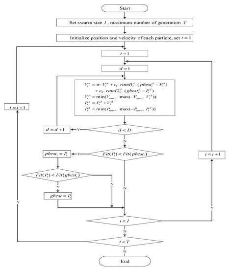
Figure 1.
Flowchart of the PSO algorithm.
3. Proposed PSO-Based SES Modeling Strategy
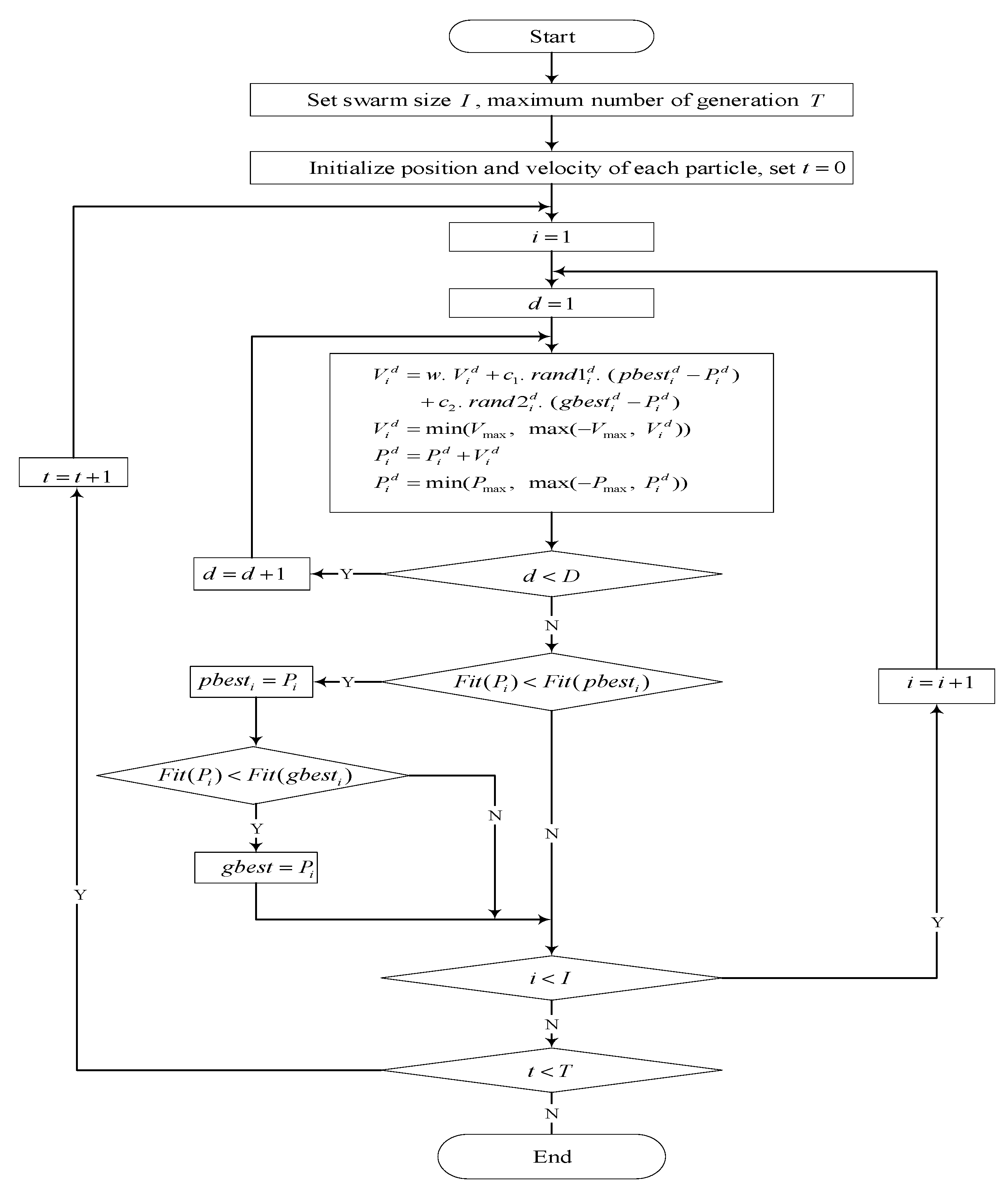
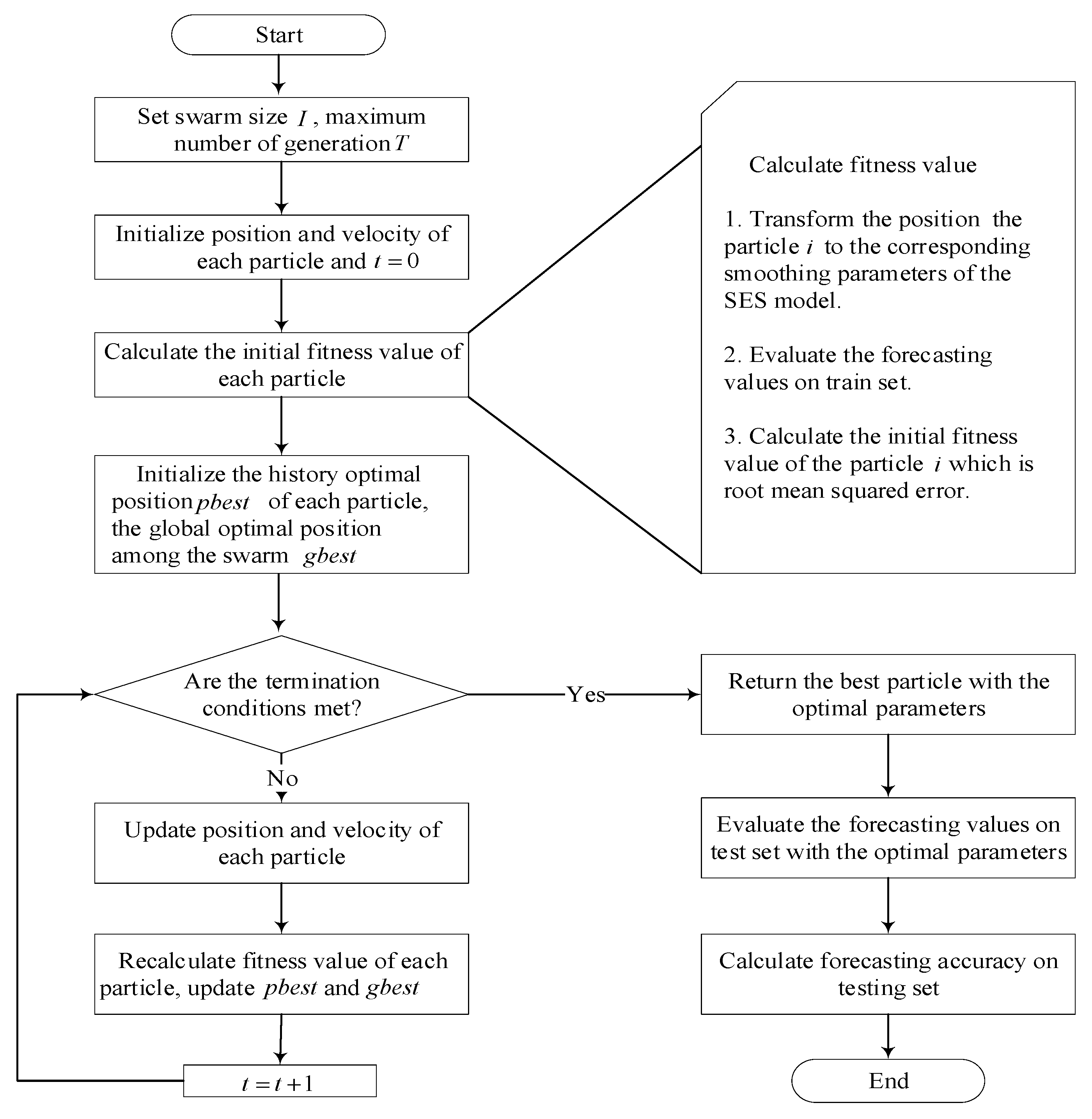
In this section, the proposed PSO-based SES modeling framework is formulated and corresponding steps involved are presented in detail, and the specific flowchart is shown in Figure 2.

Figure 2.
Flowchart of the PSO-based SES modeling strategy.
As shown in Figure 2, the detailed PSO-based SES modeling strategy includes four major operations: initialization, evaluation, update, and prediction. The overall learning process in Figure 2 is elaborated step by step below.
- Initialization
In PSO, the initial positions of all the particles are randomly distributed across a designed D-dimensional space and each dimension corresponds to a specified smoothing parameter. The initial velocity of each particle in the swarm is randomly assigned a real value which is equal to the product of a real random number uniformly distributed between 0 and 1 and the maximum velocity ; here, was usually set at 10–20% of the dynamic range of the variable in each dimension [35].
As mentioned in Section 2.1, the estimation of the trend component at initial time involves the first two full cycles of electricity consumption data; we let , then all of the data up to time were used to calculate the initial level component , the initial trend component , and the initial season factors .
- 2.
- Evaluation
In order to elaborate the computational process of the initial fitness value of each particle, we take the i-th particle and steps ahead forecast as an example, and assume that the data on the training set range from to . Firstly, the position of the i-th particle is transformed to the corresponding smoothing parameter of the SES models. Secondly, the corresponding and the prediction value at each period are calculated using the equations of the SES models and the corresponding forecasting formula, respectively. Thirdly, the fitness value is evaluated as defined in Equation (8). Finally, the current positions of all the particles are used to initialize their , and the best position visited by the entire swarm is used to initialize the .
- 3.
- Update
The position and velocity of each particle are updated using Equations (4) and (5), respectively, and their fitness values are recalculated as per Step 2. Once the fitness values of all the particles are obtained, and are updated. A judgement is made as to whether the termination condition is satisfied and, if so, the best particle with the near-optimal smoothing parameters is returned; otherwise, the previous step is repeated.
- 4.
- Prediction
The forecasting values on the test set are evaluated with the near-optimal smoothing parameters. Assuming that the data in the test set range from to , then the length of the test set is . Consistent with the prediction operation of the training set, the test set still takes periods ahead to forecast. The corresponding and the prediction value at each period are then calculated using the equations of the SES models and the corresponding forecasting formula, respectively.
4. Experimental Setup
4.1. Data Description
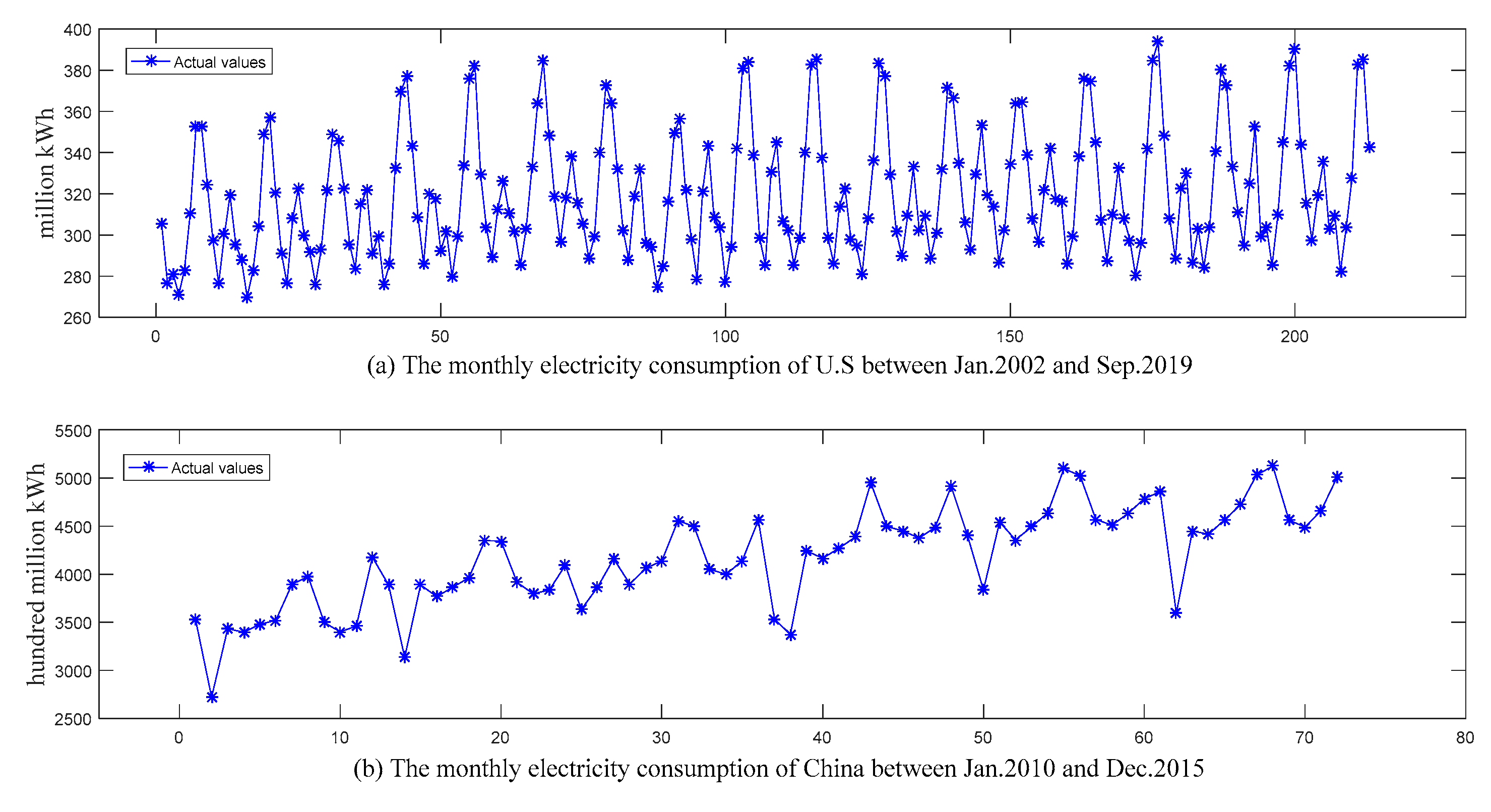
To examine the performances of the proposed PSO-based SES methods in terms of their forecast accuracy, two real-world datasets, i.e., monthly electricity consumption data from United States and China, were used in the present study. The period of the first dataset ranged from January 2002 to September 2019 and that of the second dataset was from January 2010 to December 2015.
As there are 12 months in a full period, the estimation of the trend component at initial time involved the first two full cycles of historical electricity consumption data. Therefore, the first dataset was divided into the calculation set (the first two years) used to evaluate the initialized relevant parameters in the SES models, the training set (January 2004 to December 2015), and the testing set (the last 45 months). Analogously, the second dataset was divided into the calculation set (January 2010 to December 2011), the training set (January 2012 to December 2014), and the testing set (the last 12 months in 2015). Here, the testing sets were completely independent of the training sets and were not involved in the learning procedure. Figure 3 depicts the two datasets.

Figure 3.
The monthly electricity consumption of the U.S and China.
4.2. Experimental Design
There were two goals in the experimental study. The first goal was to verify the benefits of the PSO algorithm for parameter optimization in SES models. To achieve the goal, the Holt–Winters additive model, as a popular seasonal exponential smoothing model, was employed to forecast the electricity consumption in the above two datasets, and the commonly used GS and GA were also used to optimize the parameters of the Holt–Winters additive model for comparison with PSO. The second goal was to examine the performance of the proposed PSO-based SES models and to determine which of the three different additive SES models was the most effective in terms of accuracy. In this regard, seasonal ARIMA (SARIMA) from time series forecasting models as well as SVR and a back propagation neural network model (BPNN) based on machine learning techniques were used for comparative analysis with the PSO-based SES models.
4.3. Performance Measure
To assess the forecasting performance of a model, three alternative forecasting accuracy measures were employed in this study, namely the mean absolute percentage error (MAPE) [19], the root mean square error (RMSE) [36], and the normalized root mean square error (NRMSE) [37]. Definitions of these measures are presented in the following expressions (7)–(9).
where is the sample number in the test set, is the actual value at period , and is the prediction value at period . The smaller the three measure values are, the better the prediction performance of the model.
5. Results and Discussion
5.1. Study 1: Examination of the PSO Algorithm for Parameter Optimization in SES Models
To confirm the benefit of the PSO algorithm for parameter selection in SES models, in this paper, the GS method from the classical domain and the genetic algorithm (GA) from the class of evolutionary computation were used for comparative analysis, and the quantitative and comprehensive assessments were performed with two real-world electricity consumption datasets on the basis of the prediction accuracy and computational cost for GS, GA, and PSO. The experiments were implemented in MATLAB 2016a using in-house software executed on a computer with Intel Core i5–3230M, 2.60 GHz CPU, 4 GB RAM. In general, the experimental facility did not require high computer configuration; was easy to operate, simple, and efficient; and produced repeatable experiments.
In these experiments, the MATLAB codes for GS and PSO were written in source code, while the implementation of GA used the GA toolbox that comes with MATLAB 2016a. It should be noted that the selection of parameters in the PSO algorithm (i.e., inertial weight, coefficients, swarm size, and number of iterations) is yet another challenging model selection task. The final parameters, chosen according to relative empirical and theoretical studies [32,38] and a trial-and-error approach based on the prediction performance and computational time, are summarized in Table 1. Aimed at the random of PSO algorithm, the modeling process for each prediction horizon was repeated 10 times and performance of the PSO-based additive Holt–Winters model was judged by the mean of each accuracy measure.

Table 1.
Parameter selection in PSO.
Table 2 shows the prediction performance of the additive Holt–Winters model with GS, PSO, and GA in terms of three accuracy measures (i.e., MAPE, RMSE, NRMSE) for the U.S. and China datasets. The columns labeled “Average 1—h” show the accuracy measures over the prediction horizon 1 to h. The last column shows the average ranking for each method over all forecast horizons of the out-of-sample prediction performance.
Table 2.
Prediction accuracy measures and elapsed time of GS, PSO, and GA for the U.S. and China datasets.
As per the results presented in Table 2, it was not difficult to make the following observation: when considering the U.S. dataset, GA performed the worst across three measures and the computation time was the longest. GS(0.05) and PSO had the same ranking in the terms of RMSE, and the average RMSE measures of GS(0.05) and PSO over all forecast horizons were 8.333 and 8.339, respectively. The ranking with respect to MAPE was GS(0.05) then PSO, while the ranking with respect to NRMSE was PSO then GS(0.05). Additionally, the elapsed time of GS(0.05) for a single replicate was more than twice that of PSO. When considering the China dataset, GS(0.05) performed the worst and GA performed the second worst across three measures according to the average rank. The ranking with respect to MAPE was GS(0.01) then PSO, while the ranking with respect to RMSE and NRMSE was PSO then GS(0.01). In terms of the elapsed time, the GA was computationally much more expensive than the other methods. The GS(0.05) was tens of times faster than GS(0.01), and PSO is hundreds of times faster than GS(0.01).
In conclusion, the PSO was significantly superior to GA, GS(0.01), and GS(0.05) in terms of the elapsed time. PSO outperformed GA across three measures for the majority of prediction horizons in the U.S. and China datasets. PSO was consistently better than GS(0.05) across three measures at all forecast horizons for the China dataset. Moreover, there was no significant difference between PSO and GS(0.01) for the China dataset. Thus, it is conceivable that PSO algorithm is suitable for parameter optimization in SES models.
5.2. Study 2: Comparison with Well-Known Forecasting Models
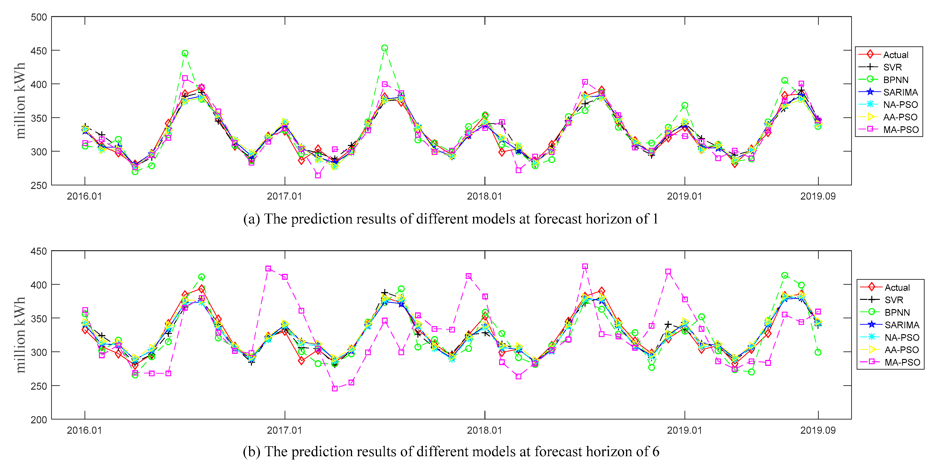
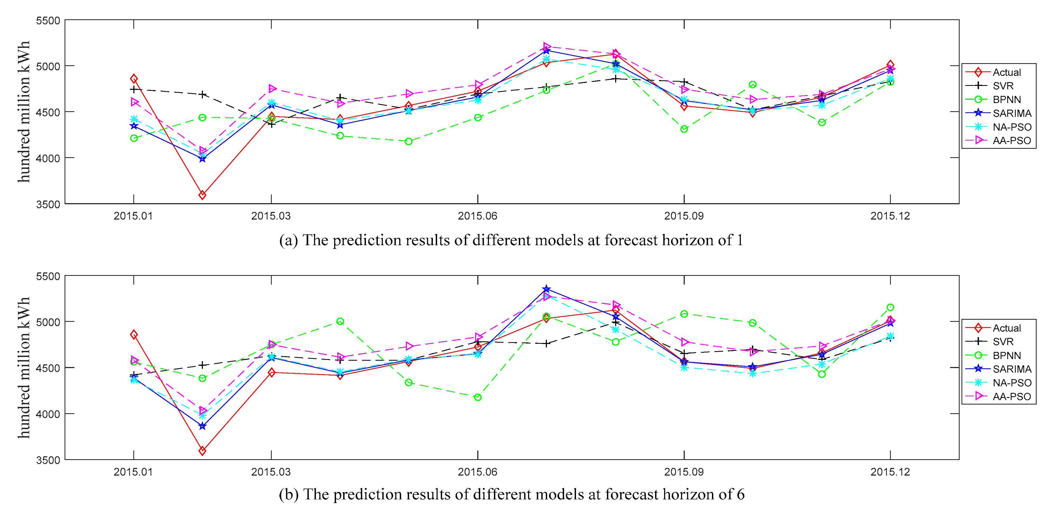
Figure 4 and Figure 5, respectively, show the comparison of actual values and predicted values for all the examined models (i.e., NA-PSO, AA-PSO, MA-PSO, SARIMA, SVR, and BPNN) in the U.S. and China datasets. And the subgraphs (a) and (b) in these two figures show the predicted values of all the examined models at the forecast horizons of 1 and 6, respectively. The prediction performances of the above models in terms of two accuracy measures (i.e., MAPE and NRMSE) are shown in Table 3. Here, “NA” denotes the SES model without a trend term but with an additive seasonal term, “AA” denotes the SES model with an additive trend term and additive seasonal term, and “MA” denotes the SES model with a multiplicative trend term and an additive seasonal term, and PSO was used to optimize the smoothing parameters of these SES models.
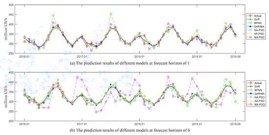
Figure 4.
The forecasted values of all the examined models at forecast horizons of 1 and 6 in the U.S. dataset.
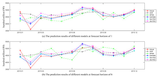
Figure 5.
The forecasted values of all the examined models at forecast horizons of 1 and 6 in the China dataset.
Table 3.
Prediction accuracy measures for the U.S. and China datasets.
The experiments of the SARIMA model were implemented in Eviews 8. The specific process was as follows:
- Stationarity test: a seasonal difference and a nonseasonal difference were performed for the original series. The augmented Dickey–Fuller test result showed that the difference series was stationary, so and ;
- model identification: the correlation coefficient graph of the difference sequence was analyzed and then the value range of ,,, and was determined;
- model selection: the trial-and-error method based on BIC was used to determine the order of the model. In this paper, the models established for the two electricity consumption datasets in U.S. and China were and , respectively, and all the estimated parameters in these two models passed the significance test;
- Residual error test: the series correlation LM test was performed on the fitted residual sequences of the above two models. The results showed that the two residual sequences were not correlated, which indicates that the models we established were credible;
- Prediction: Eviews 8 provided a dynamic forecast function for SARIMA’s multi-step-ahead prediction. Here, we obtained the predicted values of each sample in the test set from one step ahead to twelve steps ahead by changing the range of prediction sample, and then rearranged these prediction values according to the forecast horizon and further calculated the prediction accuracy of SARIMA at each forecast horizon.
The experiments of SVR and BPNN models were implemented using LibSVM toolbox (version 2.86) and BPNN toolbox in MATLAB 2016a. The parameters of SVR took default values and the embedding dimensions of SVR and BPNN were determined to be 6 and 12 by trial and error.
According to the results presented in Figure 4 and Table 3, we can make several observations about the U.S. dataset:
- Among all the examined models, the two models with the worst prediction results were MA-PSO and BPNN, which is obvious in Figure 4b.
- According to the average rank in terms of MAPE measure, the top three models turned out to be NA-PSO, then AA-PSO, and then SARIMA. The rankings with respect to NRMSE measure were SARIMA, then NA-PSO, and then AA-PSO. However, the average NRMSE measure of NA-PSO over all forecast horizons was less than that of SARIMA, which indicates that NA-PSO outperformed SARIMA to a certain extent.
- The proposed NA-PSO and AA-PSO consistently achieved more accurate forecasts than the MA-PSO regardless of the accuracy measures and forecast horizon considered. A possible reason is that multiplication form was not suitable for fitting the trend term of current electricity consumption data.
- As far as the comparison between the NA-PSO, AA-PSO, and SARIMA, we can see that the results were mixed among the horizons examined; there was an interesting phenomenon observed that whatever the accuracy measures considered, SARIMA won for one-step-ahead and two-step-ahead predictions. The main reason could be that the principle of SARIMA for multi-step-ahead prediction is recursive forecasting, which will cause errors to accumulate as the forecast horizon increases.
- Among all the examined models, the two models with the worst prediction results were SVR and BPNN, which is obvious in Figure 5a,b. The possible reason is that the methods based on machine learning were suitable for sufficient training samples, while there were only 72 samples in China dataset.
- According to the MAPE, the top three models turned out to be SARIMA, then NA-PSO, and then AA-PSO. The rankings with respect to the NRMSE measure were NA-PSO, and then AA-PSO and SARIMA tied for second. It should be noted that the reason why MA-PSO is not presented in Table 3 and Figure 5 for the China dataset is the MA-PSO performed the worst regardless of the accuracy measures and forecast horizon considered.
- As far as the comparison between the NA-PSO, AA-PSO, and SARIMA, we saw that the results were mixed among the horizons examined, but SARIMA won for one-step-ahead prediction regardless of the accuracy measures considered, which indicates that SARIMA is suitable for short-term forecasting.
- Overall, it is clear that the proposed NA-PSO held one of the top positions. The main reason could be that the electricity consumption associated with people’s daily activities and various economic activities has basically reached a saturated level, which is more intuitively reflected in Figure 3. It is not difficult to see that growth trends of electricity consumption in the U.S. and China were no longer obvious after 2005 and 2012, respectively.
In order to determine whether there existed a statistically significant difference among the five models in the hold-out sample, ANOVA procedures are performed for each performance measure, prediction horizon, and dataset. All ANOVA results were significant at the 0.05 level, which suggests that there were significant differences among the five models. The results are omitted here to save space. Tukey’s HSD test was used to further identify the significant difference between any two models. The results of these multiple comparison tests for the U.S. and China datasets are shown in Table 4. For each accuracy measure, prediction horizon, and dataset, we have ranked the models in order from 1 (the best) to 5 (the worst).
Table 4.
Multiple comparison results with ranked models for hold-out sample on U.S. and China datasets.
As per the results shown in Table 4, it is not difficult to see that the three models (i.e., NA-PSO, AA-PSO, and SARIMA) significantly outperformed SVR and BPNN in most cases, and SVR significantly outperformed BPNN in almost all cases.
When considering the U.S. dataset, the SARIMA significantly outperformed AA-PSO and NA-PSO in the cases of one-step-ahead prediction across two measures and horizon 2 for the NRMSE measure. The NA-PSO outperformed SARIMA for the overwhelming majority of prediction horizons. As far as the comparison of NA-PSO vs. AA-PSO, the NA-PSO performed significantly better than AA-PSO in most cases.
When considering the China dataset, the SARIMA significantly outperformed AA-PSO and NA-PSO in the cases of one-step-ahead prediction for MAPE measures and nine-step-ahead prediction across two measures. The AA-PSO significantly outperformed SARIMA and NA-PSO in the cases of twelve-step-ahead prediction across two measures. In addition, the NA-PSO significantly outperformed SARIMA and AA-PSO for the majority of prediction horizons.
6. Conclusions
Electricity consumption forecasting is an important issue in investment planning of electricity infrastructure, and in electricity production/generation and distribution. The purpose of this study was to perform accurate monthly electricity consumption forecasting using the proposed PSO-based SES models. The results show that PSO was significantly superior to GA and GS in terms of the elapsed time, PSO outperformed GA for the majority of predictions, and PSO and GA are almost evenly matched across three accuracy measures. Justified with the real-world electricity consumption datasets, the proposed NA-PSO and AA-PSO consistently achieved more accurate forecasts than the MA-PSO regardless of the accuracy measures and forecast horizon considered, and the three models (i.e., NA-PSO, AA-PSO, and SARIMA) significantly outperformed SVR and BPNN in most cases, and the proposed NA-PSO performed best among the three models (i.e., NA-PSO, AA-PSO, and SARIMA), which indicates that the NA-PSO could be a promised alternative for electricity consumption forecasting.
Author Contributions
Conceptualization, Y.B.; methodology, X.Z.; software, C.D. and Y.H.; validation, X.Z. and Y.H.; formal analysis, C.D.; investigation, X.Z. and C.D.; resources, Y.B.; data curation, Y.H.; writing—original draft preparation, Y.B. and X.Z.; writing—review and editing, Y.B. and Y.H.; supervision, Y.B.; funding acquisition, Y.B. All authors have read and agreed to the published version of the manuscript.
Funding
This work was funded by Humanities and Social Sciences Projects of Jiangxi under project no.GL19115, Science and Technology Research Projects of Jiangxi under project no. GJJ191188, Key R&D Projects of Jiangxi under project no.20192BBHL80015, Jiangxi Principal Academic and Technical Leaders Program under project no.20194BCJ22015, Science and Technology Research Projects of Jiangxi under project no. GJJ202905 and Natural Science Foundation of China under Project Nos. 71571080 and 71871101.
Data Availability Statement
The first data can be obtained from the website of the United States Energy Administration (https://www.eia.gov/outlooks/steo/report/electricity.php), the accessed date is October 2019 and the second data is from the literature [9].
Conflicts of Interest
The authors declare no conflict of interest.
References
- Lin, B.; Liu, C. Why is electricity consumption inconsistent with economic growth in China? Energy Policy 2016, 88, 310–316. [Google Scholar] [CrossRef]
- Kaytez, F.; Taplamacioglu, M.C.; Cam, E.; Hardalac, F. Forecasting electricity consumption: A comparison of regression analysis, neural networks and least squares support vector machines. Int. J. Electr. Power Energy Syst. 2015, 67, 431–438. [Google Scholar] [CrossRef]
- Wu, L.; Gao, X.; Xiao, Y.; Yang, Y.; Chen, X. Using a novel multi-variable grey model to forecast the electricity consumption of Shandong Province in China. Energy 2018, 157, 327–335. [Google Scholar] [CrossRef]
- Xie, W.; Wu, W.-Z.; Liu, C.; Zhao, J. Forecasting annual electricity consumption in China by employing a conformable fractional grey model in opposite direction. Energy 2020, 202, 117682. [Google Scholar] [CrossRef]
- Bianco, V.; Manca, O.; Nardini, S. Electricity consumption forecasting in Italy using linear regression models. Energy 2009, 34, 1413–1421. [Google Scholar] [CrossRef]
- Vu, D.H.; Muttaqi, K.M.; Agalgaonkar, A. A variance inflation factor and backward elimination based robust regression model for forecasting monthly electricity demand using climatic variables. Appl. Energy 2015, 140, 385–394. [Google Scholar] [CrossRef] [Green Version]
- Yuan, J.; Farnham, C.; Azuma, C.; Emura, K. Predictive artificial neural network models to forecast the seasonal hourly electricity consumption for a University Campus. Sustain. Cities Soc. 2018, 42, 82–92. [Google Scholar] [CrossRef]
- Azadeh, A.; Ghaderi, S.; Sohrabkhani, S. A simulated-based neural network algorithm for forecasting electrical energy consumption in Iran. Energy Policy 2008, 36, 2637–2644. [Google Scholar] [CrossRef]
- Cao, G.; Wu, L. Support vector regression with fruit fly optimization algorithm for seasonal electricity consumption forecasting. Energy 2016, 115, 734–745. [Google Scholar] [CrossRef]
- Taylor, J.W. Short-term electricity demand forecasting using double seasonal exponential smoothing. J. Oper. Res. Soc. 2003, 54, 799–805. [Google Scholar] [CrossRef]
- Bianco, V.; Manca, O.; Nardini, S.; Minea, A.A. Analysis and forecasting of nonresidential electricity consumption in Romania. Appl. Energy 2010, 87, 3584–3590. [Google Scholar]
- Hussain, A.; Rahman, M.; Memon, J.A. Forecasting electricity consumption in Pakistan: The way forward. Energy Policy 2016, 90, 73–80. [Google Scholar] [CrossRef]
- Kialashaki, A.; Reisel, J.R. Development and validation of artificial neural network models of the energy demand in the industrial sector of the United States. Energy 2014, 76, 749–760. [Google Scholar] [CrossRef]
- Shen, M.; Sun, H.; Lu, Y. Household Electricity Consumption Prediction Under Multiple Behavioural Intervention Strategies Using Support Vector Regression. Energy Procedia 2017, 142, 2734–2739. [Google Scholar] [CrossRef]
- Hernández, L.; Baladrón, C.; Aguiar, J.M.; Calavia, L.; Lloret, J. Experimental Analysis of the Input Variables’ Relevance to Forecast Next Day’s Aggregated Electric Demand Using Neural Networks. Energies 2013, 6, 2927–2948. [Google Scholar] [CrossRef]
- Khosravi, A.; Nahavandi, S.; Creighton, D.; Srinivasan, D. Interval Type-2 Fuzzy Logic Systems for Load Forecasting: A Comparative Study. IEEE Trans. Power Syst. 2012, 27, 1274–1282. [Google Scholar] [CrossRef]
- Xiao, X.; Yang, J.; Mao, S.; Wen, J. An improved seasonal rolling grey forecasting model using a cycle truncation accumulated generating operation for traffic flow. Appl. Math. Model. 2017, 51, 386–404. [Google Scholar] [CrossRef]
- Khuntia, S.R.; Rueda, J.L.; van Der Meijden, M.A. Forecasting the load of electrical power systems in mid- and long-term horizons: A review. IET Gener. Transm. Distrib. 2016, 10, 3971–3977. [Google Scholar] [CrossRef] [Green Version]
- Jiang, W.; Wu, X.; Gong, Y.; Yu, W.; Zhong, X. Holt–Winters smoothing enhanced by fruit fly optimization algorithm to forecast monthly electricity consumption. Energy 2020, 193, 116779. [Google Scholar] [CrossRef]
- Taylor, J.W. An evaluation of methods for very short-term load forecasting using minute-by-minute British data. Int. J. Forecast. 2008, 24, 645–658. [Google Scholar] [CrossRef]
- Tratar, L.F.; Strmcnik, E. The comparison of Holt–Winters method and Multiple regression method: A case study. Energy 2016, 109, 266–276. [Google Scholar] [CrossRef]
- Tiao, G.C.; Xu, D. Robustness of maximum likelihood estimates for multi-step predictions: The exponential smoothing case. Biometrika 1993, 80, 623–641. [Google Scholar] [CrossRef]
- Ord, J.K.; Koehler, A.B.; Snyder, R.D. Estimation and prediction for a class of dynamic nonlinear statistical models. J. Am. Stat. Assoc. 1997, 92, 1621–1629. [Google Scholar] [CrossRef]
- Broze, L.; Melard, G. Exponential smoothing: Estimation by maximum likelihood. J. Forecast. 1990, 9, 445–455. [Google Scholar] [CrossRef]
- Hyndman, R.J.; Koehler, A.B.; Ord, J.K.; Snyder, R.D. Prediction intervals for exponential smoothing using two new classes of state space models. J. Forecast. 2005, 24, 17–37. [Google Scholar] [CrossRef]
- Zhang, X.-L.; Zhao, J.-H.; Cai, B. Prediction model with dynamic adjustment for single time series of PM2.5. Acta Autom. Sin. 2018, 44, 1790–1798. [Google Scholar]
- Hong, W.-C. Chaotic particle swarm optimization algorithm in a support vector regression electric load forecasting model. Energy Convers. Manag. 2009, 50, 105–117. [Google Scholar] [CrossRef]
- AlRashidi, M.; El-Naggar, K. Long term electric load forecasting based on particle swarm optimization. Appl. Energy 2010, 87, 320–326. [Google Scholar] [CrossRef]
- Hu, Z.; Bao, Y.; Xiong, T. Comprehensive learning particle swarm optimization based memetic algorithm for model selection in short-term load forecasting using support vector regression. Appl. Soft Comput. 2014, 25, 15–25. [Google Scholar] [CrossRef]
- Yang, Y.; Shang, Z.; Chen, Y.; Chen, Y. Multi-Objective Particle Swarm Optimization Algorithm for Multi-Step Electric Load Forecasting. Energies 2020, 13, 532. [Google Scholar] [CrossRef] [Green Version]
- Kennedy, J.; Eberhart, R. Particle Swarm Optimization. In Proceedings of the ICNN’95—International Conference on Neural Networks, Perth, WA, Australia, 27 November–1 December 1995. [Google Scholar]
- Trelea, I.C. The particle swarm optimization algorithm: Convergence analysis and parameter selection. Inf. Process. Lett. 2003, 85, 317–325. [Google Scholar] [CrossRef]
- Hyndman, R.J.; Koehler, A.B.; Snyder, R.D.; Grose, S. A state space framework for automatic forecasting using exponential smoothing methods. Int. J. Forecast. 2002, 18, 439–454. [Google Scholar] [CrossRef] [Green Version]
- Han, F.; Ling, Q.H. A new approach for function approximation incorporating adaptive particle swarm optimization and a priori information. Appl. Math. Comput. 2008, 205, 792–798. [Google Scholar] [CrossRef]
- Shi, Y. Particle Swarm Optimization: Developments, Applications and Resources. In Proceedings of the 2001 Congress on Evolutionary Computation (IEEE Cat. No. 01TH8546), Seoul, Korea, 27–30 May 2001; pp. 81–86. [Google Scholar]
- Willmott, C.J.; Matsuura, K. Advantages of the mean absolute error (MAE) over the root mean square error (RMSE) in assessing average model performance. Clim. Res. 2005, 30, 79–82. [Google Scholar] [CrossRef]
- Lawal, A.S.; Servadio, J.L.; Davis, T.; Ramaswami, A.; Botchwey, N.; Russell, A.G. Orthogonalization and machine learning methods for residential energy estimation with social and economic indicators. Appl. Energy 2021, 283, 116114. [Google Scholar] [CrossRef]
- Chen, Y.P.; Peng, W.C. Particle Swarm Optimization With Recombination and Dynamic Linkage Discovery. IEEE Trans. Syst Man Cybern. B Cybern. 2007, 37, 1460–1470. [Google Scholar] [CrossRef]
Publisher’s Note: MDPI stays neutral with regard to jurisdictional claims in published maps and institutional affiliations. |
© 2021 by the authors. Licensee MDPI, Basel, Switzerland. This article is an open access article distributed under the terms and conditions of the Creative Commons Attribution (CC BY) license (https://creativecommons.org/licenses/by/4.0/).