Numerical Modelling on CO2 Storage Capacity in Depleted Gas Reservoirs

Akai, Takashi; Saito, Naoki; Hiyama, Michiharu; Okabe, Hiroshi

doi:10.3390/en14133978

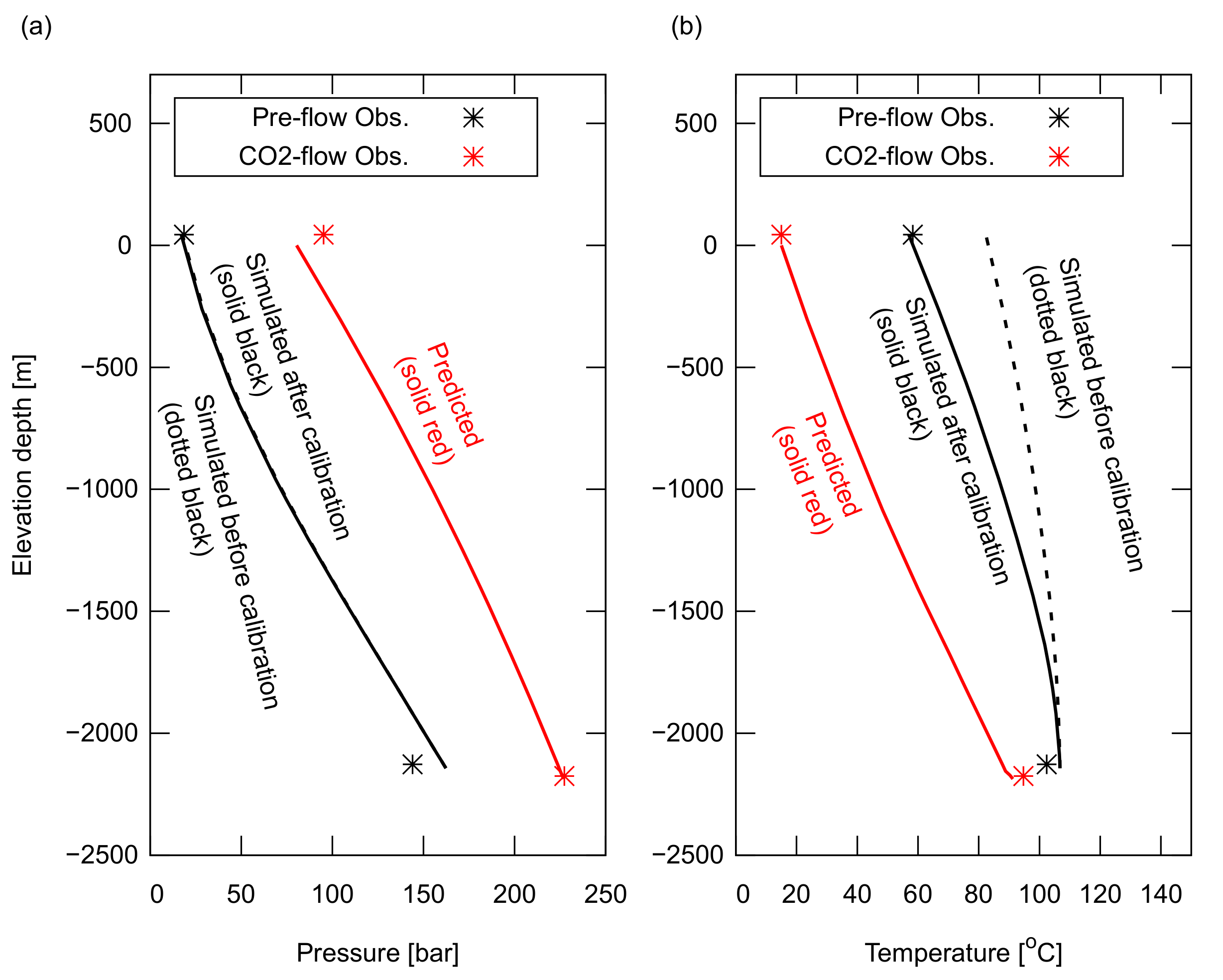
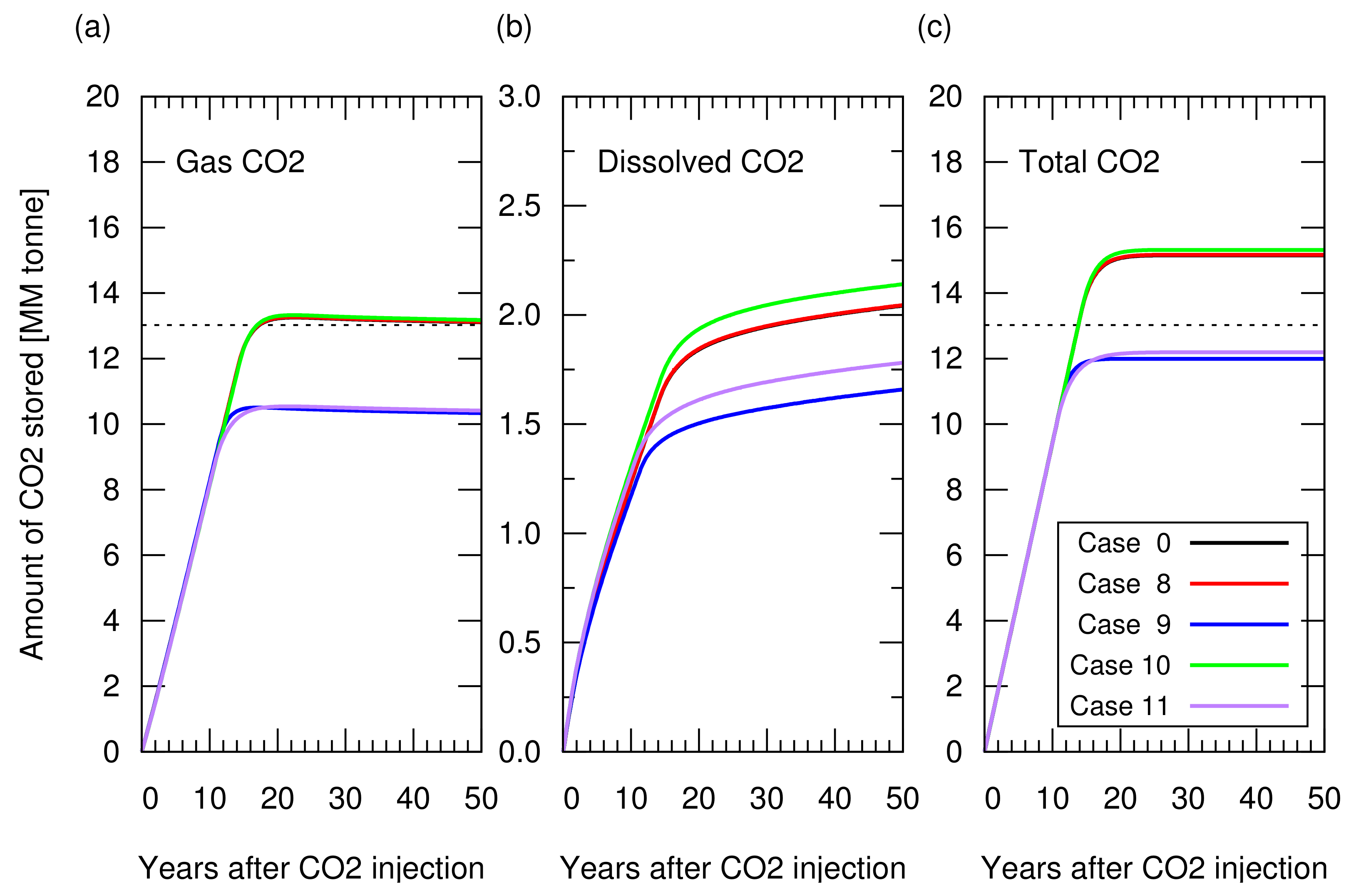
Open AccessArticle

Numerical Modelling on CO₂ Storage Capacity in Depleted Gas Reservoirs

Japan Oil, Gas and Metals National Corporation (JOGMEC), Tokyo 105-0001, Japan

^*

Author to whom correspondence should be addressed.

Energies 2021, 14(13), 3978; https://doi.org/10.3390/en14133978

Submission received: 2 June 2021 / Revised: 18 June 2021 / Accepted: 25 June 2021 / Published: 2 July 2021

Download

Browse Figures

Versions Notes

Abstract

:

Making an accurate estimate of the CO

_{2}

storage capacity before the commencement of a carbon capture and storage (CCS) project is crucial to the project design and feasibility investigation. We present herein a numerical modelling study on the CO

_{2}

storage capacity in depleted gas reservoirs. First, we show a simple volumetric equation that gives the CO

_{2}

storage capacity in a depleted gas reservoir, which considers the same volume of CH

_{4}

at reservoir pressure and temperature conditions produced from the reservoir. Next, the validity and the limitations of this equation are investigated using a numerical reservoir simulation with the various reservoir characteristics of reservoir heterogeneity, aquifer water encroachment, and rock compaction and its reversibility. Regardless of the reservoir heterogeneity, if a reservoir is subjected to a weak or moderate aquifer support, the volumetric equation provides an estimate of the CO

_{2}

storage capacity as structurally trapped gas within 1% of that estimated from numerical simulations. The most significant factor influencing the CO

_{2}

storage capacity is the reversibility of rock compaction, rather than the degree of rock compaction. If reservoir rocks have a strong hysteresis in their compaction and expansion behaviour, the material balance equation will overestimate the amount of structural CO

_{2}

trapping. All the simulation results show a fairly consistent amount of trapped CO

_{2}

as a dissolved component in water, which is 15∼17% of the structurally trapped CO

_{2}

. Overall, our study presents the validity and the limitation of the simple material balance equation for estimating the CO

_{2}

storage capacity, which helps with designing a CCS project at the early stage.

Keywords:

carbon capture and storage (CCS); CO2 injection in depleted gas reservoirs; reservoir hysteresis; compositional simulation

Graphical Abstract

1. Introduction

The development of natural resources has recently seen an increasing demand for decarbonization, which reduces or eliminates carbon dioxide (CO

_{2}

) from energy sources. Having a good affinity for the development of natural resources, CO

_{2}

capture and storage (CCS) in underground geological formations is one of the most promising ways to decarbonaize because, it uses technologies developed for and applied by the natural resources industry.

Three types of geological formation are suitable for CCS: deep saline formations, depleted oil and gas reservoirs, and unminable coal beds [1]. The CO

_{2}

injected into these geological formations is securely trapped via the following four major mechanisms: structural (hydrostratigraphic), residual (capillary), solubility, and mineral trapping [2,3]. The first two mechanisms are classified as physical trapping, whereas the latter two are classified as geochemical trapping [3]. The significance of each mechanism depends on the type of geological formation and its changes over time [4]. Generally speaking, physical trapping occurs over a time period of 10∼100 years, while geochemical trapping takes effect over a longer time period of >100 years [1,4].

Among these geological formations, depleted oil and gas reservoirs are often considered the best option [5,6] because: (a) they have sufficient storage potential worldwide [1]; (b) the information on subsurface reservoirs collected during the hydrocarbon reservoir development could reduce the uncertainty in a CCS project; and (c) using existing infrastructure for the hydrocarbon development could make a CCS project economically more favorable compared to other options [6].

This study focuses on CO

_{2}

injection into depleted gas reservoirs, specifically dry gas reservoirs, where injected CO

_{2}

mixes with the remaining hydrocarbon gas in depressurized reservoirs and is primarily stored as a structurally trapped gas. In this case, a simple material balance between produced hydrocarbon gas and the CO

_{2}

to be injected should provide a good approximation of the CO

_{2}

storage capacity. If this is the case, this material balance estimation is quite useful at the early stage of CCS project design because this estimation essentially only requires information about initial reservoir pressure and temperature conditions and cumulative gas production during the history of hydrocarbon gas production; this is some of the most accurate information pertaining to the subsurface reservoir of interest. Although many studies have presented the CO

_{2}

storage capacity of particular depleted gas reservoirs based on a numerical simulation [6,7,8], to what extent this material balance produces an acceptable estimation of the CO

_{2}

storage capacity under various reservoir conditions is not well understood.

Hence, this study investigates the validity and the limitations of the simple material balance estimation of the CO

_{2}

storage capacity for several realistic conditions of reservoir heterogeneity, aquifer water encroachment, and rock compaction. We use numerical reservoir simulations to obtain the CO

_{2}

storage capacity under various reservoir conditions. The resultant amount of CO

_{2}

stored in the reservoir is then compared with the CO

_{2}

storage capacity estimated from the simple material balance.

The remainder of this paper is organized as follows: Section 2.1 presents a simple material balance equation originally proposed by Bachu et al. [9], which gives the CO

_{2}

storage capacity in a depleted gas reservoir; Section 3 presents a comparison between the amount of stored CO

_{2}

obtained with the numerical simulations and estimated from the volumetric equation; and Section 4 discusses the implications of our findings for practical CCS projects.

2. Methods

2.1. Volumetric Estimation of CO $_{2}$ Storage Capacity

The gas volume factor of a component X,

B_{g}^{X}

, is given as follows based on the equation of state of real gases:

\begin{matrix} B_{g}^{X} = \frac{V_{R}}{V_{S}} = \frac{P_{S}}{P_{R}} \frac{T_{R}}{T_{S}} \frac{z_{R}^{X}}{z_{S}^{X}}, \end{matrix}

(1)

where V, P, T and z are the volume, pressure, temperature and z-factor (compressibility factor), respectively, and subscripts R and S denote the reservoir and standard conditions (15

^{\circ}

C and 1 Bar), respectively.

We consider the volume of CH

_{4}

at the standard condition,

V_{S}^{{CH}_{4}}

. This can be the amount of CH

_{4}

produced by a reservoir. At the reservoir condition, this CH

_{4}

occupies the following volume:

V_{R}^{{CH}_{4}} = V_{S}^{{CH}_{4}} B_{g}^{{CH}_{4}} .

(2)

Hence, the same CO

_{2}

volume that can be stored in the reservoir,

V_{S}^{{CO}_{2}}

, can be calculated as follows:

\begin{matrix} V_{S}^{{CO}_{2}} & = & \frac{V_{R}^{{CO}_{2}}}{B_{g}^{{CO}_{2}}}, \end{matrix}

(3)

\begin{matrix} = & \frac{V_{R}^{{CH}_{4}}}{B_{g}^{{CO}_{2}}}, \end{matrix}

(4)

\begin{matrix} = & \frac{B_{g}^{{CH}_{4}}}{B_{g}^{{CO}_{2}}} V_{S}^{{CH}_{4}} . \end{matrix}

(5)

Here, we used

V_{R}^{{CH}_{4}} = V_{R}^{{CO}_{2}}

. Finally, using Equation (1) and

z_{s}^{X} = 1

, we obtain:

V_{S}^{{CO}_{2}} = \frac{z_{R}^{{CH}_{4}}}{z_{R}^{{CO}_{2}}} V_{S}^{{CH}_{4}} .

(6)

The volume of CO

_{2}

storage capacity estimated with this equation will be compared with the amount of stored CO

_{2}

computed from the numerical simulations in Section 3.

2.2. Numerical Model Descriptions

The ECLIPSE compositional simulator, a commercial reservoir simulator, was used. The mass conservation of each component is given by

\begin{matrix} \frac{d M_{i}}{d t} + \nabla M_{i} + Q_{i} = 0, \end{matrix}

(7)

where the first term denotes net mass accumulation of component i; the second term denotes net mass flux; and the third term denotes source and sink terms. The simulator solves this differential equation based on finite difference methods (FDM). The second term, the net mass flux term, is determined from multiphase Darcy’s law, which is described as:

\begin{matrix} q_{p} = - \frac{k k_{r p}}{μ_{p}} (\nabla P_{p} - ρ_{p} g), \end{matrix}

(8)

where the subscript p denotes phase p; q is the Darcy velocity; k and

k_{r}

are the absolute and relative permeability, respectively;

ρ

and

μ

are the density and viscosity, respectively; P is the hydrodynamic pressure; and

g

is the gravitational acceleration. More details on the numerical schemes of the simulator can be found in [10,11].

In this study, we considered the three components of CH

_{4}

, CO

_{2}

and water (aqueous phase) to model CO

_{2}

injection in depleted dry gas reservoirs. In this numerical model, the phase separation of the components was modelled based on the modified Peng Robinson equation, proposed by Søreide and Whitson [12], to obtain accurate gas solubilities in the aqueous phase [11]. Hence, both CH

_{4}

and CO

_{2}

can be present in the aqueous phase as a dissolved component in water. In addition to mass transport by Darcy’s law, we modelled the diffusive mass transport of components in both the gas and aqueous phases based on Fick’s second law [4]. The diffusion coefficient, D, for the components in the gas and aqueous phases was set to 1.2

\times 10^{- 7}

m

^{2}

/s and 1.2

\times 10^{- 9}

m

^{2}

/s, respectively, based on the typical values for the molecular diffusion coefficient of the components in the gas and water phases [13].

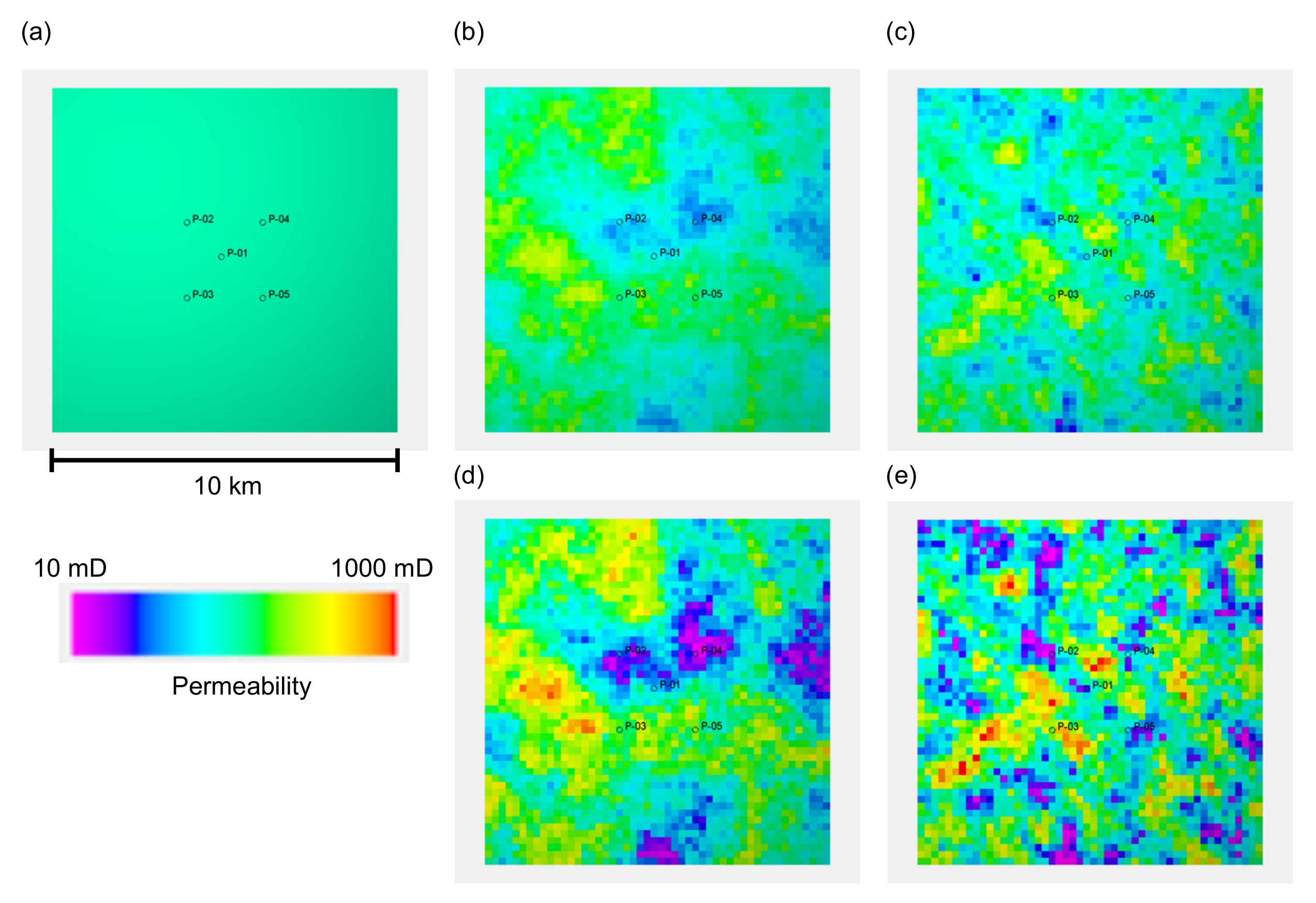
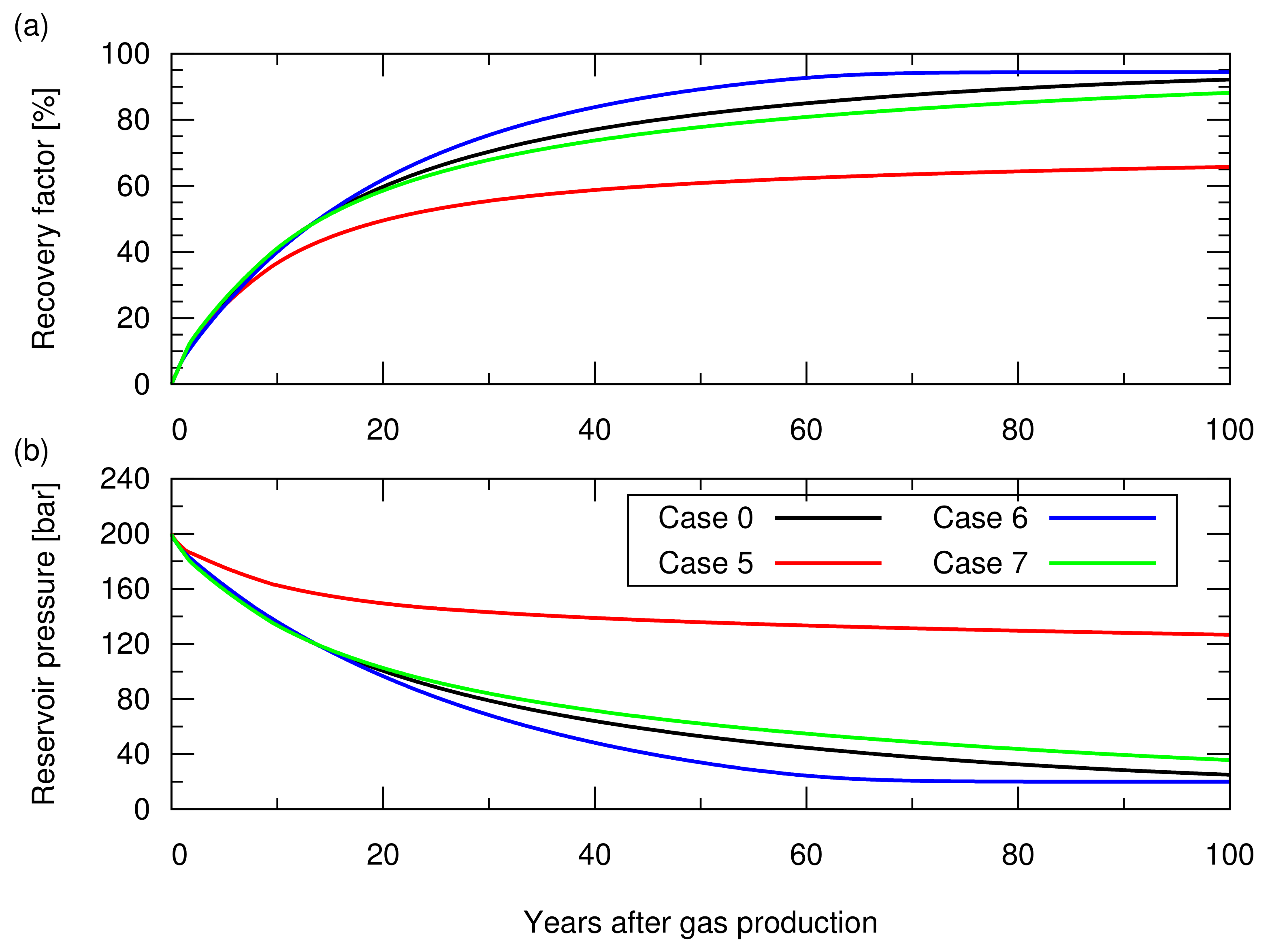
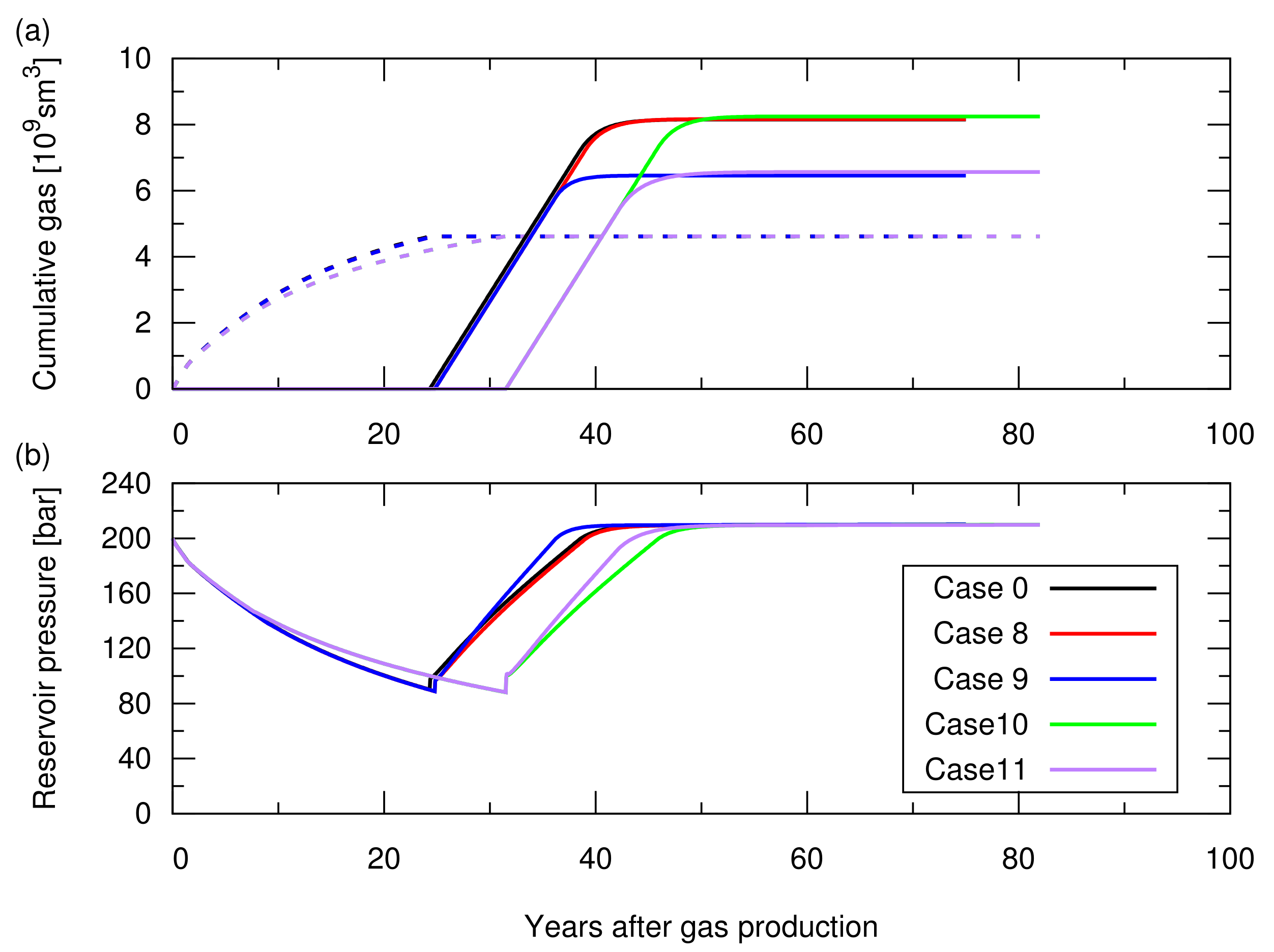
A four-way closure reservoir model, with the spherical shape of a reservoir top surface that had a horizontal extent of 10 km in the x and y directions, was used. A sand body with a uniform thickness of 50 m was considered as a reservoir sand. A cap rock layer with a uniform thickness of 5 m was modelled immediately above the reservoir section. This structure was modelled with a grid block with a size of 200 m × 200 m × 1 m, which resulted in 50 × 50 × 55 grid blocks. The depth of the reservoir top was 2000 m at the centre of the model. The gas–water contact was located at a depth of 2030 m. Hence, this gas reservoir was subjected to pressure support from the bottom aquifer below the gas–water contact. Five wells, composing a five-spot pattern with a 2 km side length, were placed in the model. These wells were completed for 10 m from the top reservoir surface. Figure 1 depicts the reservoir model and the well location.

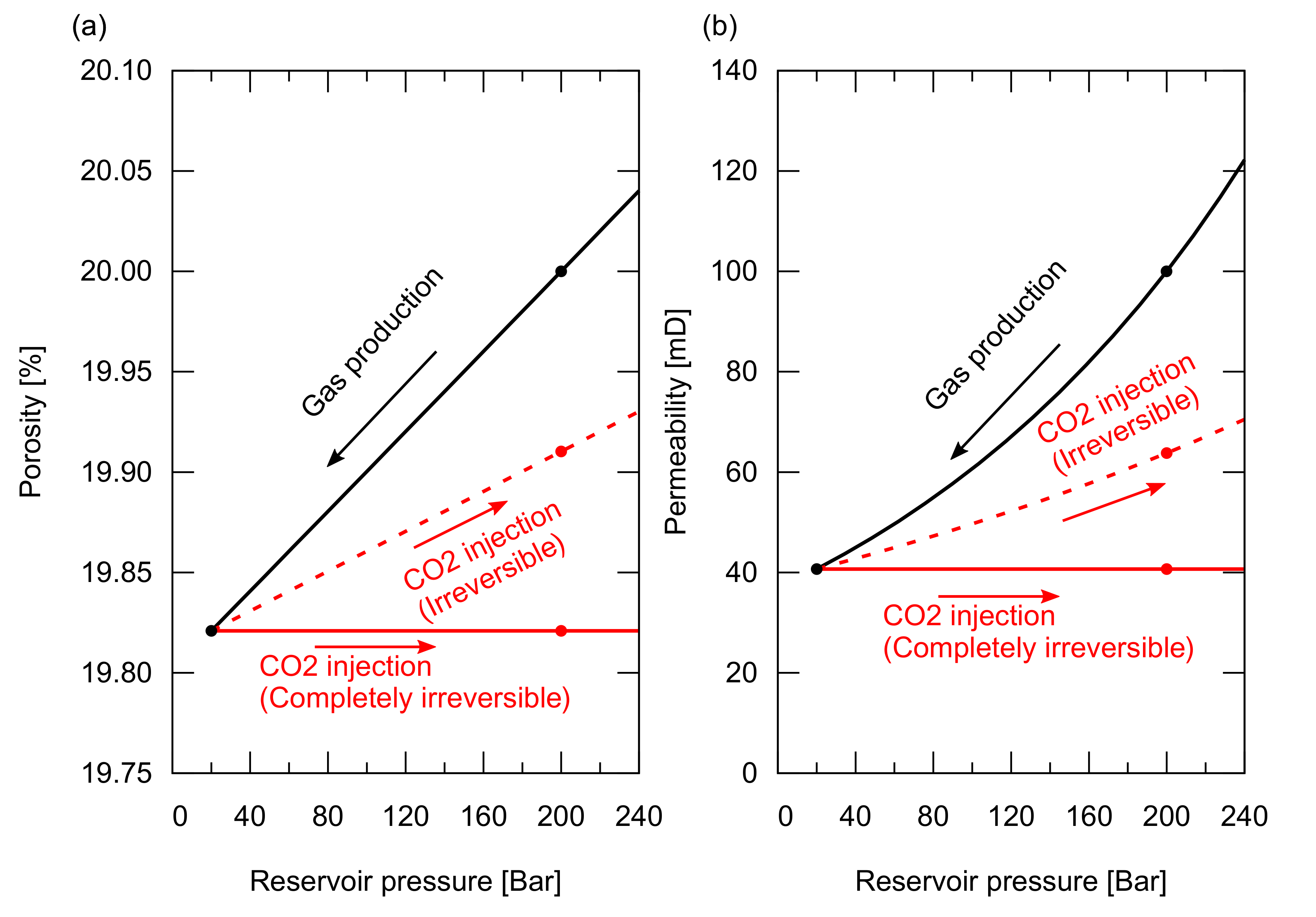
We assumed an isothermal temperature of 100

^{\circ}

C and a hydrostatic pressure of 200 Bar at a datum depth of 2015 m (initial reservoir pressure varied with depth with the water gradient). As a base case (case 0), we considered the homogeneous porosity,

ϕ

, and the permeability, k, of 20% and 100 mD, respectively. We also considered heterogeneous

ϕ

and k distributions, which will be described in Section 3.1.

For the saturation functions of the relative permeability,

k_{r}

, and the capillary pressure,

P_{c}

, of the reservoir sand, the hysteresis in drainage and imbibition was modelled as shown in Figure 2. The relative permeability of the reservoir sand was determined based on the measured data of Krevor et al. [14], preformed for a CO

_{2}

/water system on Berea sandstone samples. These relative permeability curves had a connate water saturation,

S_{w c}

, of 40% and a trapped gas saturation,

S_{g t}

of 36%. The capillary pressure curves for drainage and imbibition were modelled based on the Van Genuchten model [15]. The curve shape was determined based on the experimental data from Bottero et al. [16], while the magnitude of the pressure was adjusted to provide a reasonable capillary pressure for a sandstone with a permeability of 100 mD—the maximum capillary pressure at

S_{w c}

was 0.5 Bar, corresponding to a pore radius, R, of ∼1

μ

m for a CO

_{2}

/water system that has an interfacial tension,

σ

, of 35 mN/m and a contact angle,

θ

, of 30

^{\circ}

based on the Young–Laplace relationship:

P_{c} = 2 σ cos θ / R

. Furthermore, in Section 3.2, we investigated the impact of the hysteresis on the saturation functions by changing the value of

S_{g t}

, which will be described later.

3. Results

We studied the influence of reservoir characteristics on CO

_{2}

storage capacity. Three reservoir characteristics were chosen: reservoir heterogeneity in Section 3.1, encroachment of aquifer water in Section 3.2, and rock compaction and its reversibility in Section 3.3. Twelve reservoir simulation cases were performed with different inputs for these three characteristics. The amount of stored CO

_{2}

computed from the reservoir simulations was then compared with the volumetrically estimated CO

_{2}

storage capacity using Equation ().

3.1. Reservoir Heterogeneity

We designed five reservoir models with different porosity and permeability distributions to represent different degrees of reservoir heterogeneity, that is, one homogeneous porosity and permeability distribution, and four heterogeneous distributions. The homogeneous model had 20% porosity and 100 mD permeability. All four heterogeneous models had statistically similar porosity distributions with a mean value of 20% and a standard deviation of 4%. The spatial distribution of porosity was geostatistically determined using a sequential Gaussian simulation with different correlation lengths in the horizontal direction,

θ_{h}

, that is, 3000 m and 1000 m (the correlation length in the vertical direction of 2 m was assigned for both cases). For both porosity distributions, two types of permeability distributions were generated for each porosity distribution based on the two types of porosity and permeability relationships shown in Figure 3a. Both relationships have a permeability of 100 mD for a mean porosity of 20%. One relationship had 10 mD for 5% porosity, while the other had 30 mD for the same porosity. Figure 3b illustrates the histograms of the resultant permeability values. The permeability distributions of these five models are shown in Figure 4. Based on these models, five simulation cases were designed as summarized in Table 1.

First, we performed 100 years of hydrocarbon gas production with the five producers placed in the models. The producers were controlled by a target gas production rate of

2.83 \times 10^{5}

sm

^{3}

/d/well (∼10 MMscf/d/well) with a minimum bottom hole pressure constrain of 20 Bar, and a maximum water production rate of 15 sm

^{3}

/d/well (∼100 bbl/d/well). Figure 5 shows the simulated cumulative gas production and the reservoir pressure as a function of time. For all cases, first, the producers started production with the target gas production rate, then they showed a decline in the gas production rate when they reached the maximum water production rate constrain after the aquifer water encroachment from the bottom. Subsequently, they further reduced the gas production rate when their bottom hole pressure reached the minimum bottom hole pressure constrain. Depending on the degree of heterogeneity, they showed different gas recoveries.

Next, we performed CO

_{2}

storage simulations. In these simulations, we made a consistent comparison by starting the CO

_{2}

injection when the cumulative gas production reached

4.62 \times 10^{9}

sm

^{3}

, which accounted for 65% of the original gas in place, that is, a 65% recovery factor. CO

_{2}

was injected from the five wells placed for the gas production, while stopping gas production from these wells. These CO

_{2}

injection wells were controlled by a maximum bottom hole pressure constrain of 210 Bar, which was 5% higher than the initial reservoir pressure. With this constrain, the reservoir pressure returned to the initial reservoir at the end of the CO

_{2}

injection. Figure 6 shows the amount of stored CO

_{2}

. Figure A1 in Appendix A depicts the cumulative CH

_{4}

production and CO

_{2}

injection, and reservoir pressure for these cases. Despite the different reservoir heterogeneities, all models resulted in a similar storage amount (less than 2% difference in the total amount of CO

_{2}

storage). The amount of CO

_{2}

structurally trapped as a gas phase was consistent with the value volumetrically estimated from Equation (). A difference in the amount of CO

_{2}

stored as a dissolved component in brine was observed, but this amount was one order of magnitude lower than that of trapped CO

_{2}

as a gas phase, indicating a minor contribution to the total storage amount.

3.2. Aquifer Water Encroachment

The influence of the aquifer water encroachment on both hydrocarbon gas production and CO

_{2}

injection is considered in this section. An additional three cases, shown in Table 2, were designed. In case 5, the aquifer volume below the gas–water contact was increased from its original volume of 20 PVs to 40 PVs by increasing the pore volumes of the x and y boundary grid cells. The influence of the hysteresis of the saturation functions was considered in cases 6 and 7. In case 6, there was no hysteresis in drainage and imbibition with

S_{g t} = 0 %

. In this case, for both drainage and imbibition, the gas relative permeability and the capillary pressure followed the curves for drainage as shown in black in Figure 2. In case 7, we considered a greater hysteresis compared to that in case 0 (base case) with an increase of

S_{g t}

to 45% from its original value of 36%.

Figure 7 shows the gas recovery factor and the reservoir pressure obtained for these cases. In case 5, due to the significant invasion of aquifer water from the bottom of the reservoir, the entire reservoir section was invaded by aquifer water, leaving the residual trapped gas (

S_{g t} = 36 %

) in the entire reservoir section. Meanwhile, the reservoir pressure was maintained at a higher level than that of the other cases because of the pressure support from the aquifer water. Consequently, the recovery factor resulted in a 20% lower value than that of case 0. For cases 6 and 7, as expected, case 6, with a smaller

S_{g t}

, resulted in a higher recovery factor compared to case 0 while case 7, with a greater

S_{g t}

, resulted in a lower recovery factor. These simulations showed that the degree of aquifer water invasion and the amount of gas left in an aquifer invaded zone significantly influenced the gas recovery factor.

As described in Section 3.1, CO

_{2}

injection was started when the cumulative gas production reached

4.62 \times 10^{9}

sm

^{3}

(RF = 65%). Figure 8 shows the amount of stored CO

_{2}

. Figure A2 in Appendix A depicts the cumulative CH

_{4}

production and CO

_{2}

injection, and the reservoir pressure for these cases. Case 5 showed a 10% greater amount of structurally trapped CO

_{2}

as a gas phase, compared to the other cases, because a greater amount of aquifer water was produced in this case due to a long duration of gas production (i.e., case 5 took more than 80 years to reach 65% of RF, while the other cases reached 65% of RF less than 20 years), which provided additional space for CO

_{2}

storage. Cases 6 and 7 resulted in a similar amount of structurally trapped CO

_{2}

as that obtained with case 0, which was consistent with the amount estimated from Equation ().

3.3. Rock Compaction and Its Reversibility

The influence of rock compaction and its reversibility is considered in this section. According to Terzaghi’s principle, the effective stress,

σ^{'}

, is related to the total stress,

σ

, and the pore pressure,

P_{p}

, by the following relationship [17]

\begin{matrix} σ^{'} = σ - P_{p} . \end{matrix}

(9)

During the gas production by natural depletion, rocks undergo a compaction process caused by the decrease in pore pressure (reservoir pressure) with a constant total stress. We considered the influence of rock compaction on both pore volume and permeability based on the following exponential relationships:

\begin{matrix} C_{p} = - \frac{1}{ϕ} \frac{d ϕ}{d σ^{'}} & \Leftrightarrow & ϕ = ϕ^{r e f} exp [C_{p} (P_{p} - P_{p}^{r e f})], \end{matrix}

(10)

\begin{matrix} γ = - \frac{1}{k} \frac{d k}{d σ^{'}} & \Leftrightarrow & k = k^{r e f} exp [γ (P_{p} - P_{p}^{r e f})], \end{matrix}

(11)

where

C_{p}

and

γ

are the porosity and the permeability compressibility coefficient, respectively, and the superscript

r e f

denotes reference values. We used

ϕ^{r e f} = 20

% and

k^{r e f} = 100

mD at a reference pressure of

P_{p} = P_{i} = 200

Bar (

P_{i}

is the initial reservoir pressure). We set

C_{p} = 5 \times 10^{- 5}

bar

^{- 1}

and

γ = 5 \times 10^{- 3}

bar

^{- 1}

based on the reported values in the literature [18].

The pore pressure increases again during the CO

_{2}

injection after the gas production. The expansion trends of the porosity and the permeability do not necessarily follow the compaction trend during a depletion process. Figure 9 shows the modelled rock compaction and expansion trends for the porosity and the permeability. During the gas production, the porosity and the permeability decrease along the black line in the figure. For a reversible process, they increase along the black line during the CO

_{2}

injection, whereas for a completely irreversible process, they retain the values at the lowest reservoir pressure condition during the CO

_{2}

injection, as shown by the red lines (a partially reversible process is shown by the dotted red line).

We designed the four cases summarized in Table 3 to study the influence of rock compaction and its reversibility on gas recovery and CO

_{2}

storage. In cases 8 and 9, only porosity compaction was considered. In case 8, reversible expansion (i.e., the porosity increased following the black line in Figure 9) was considered. In case 9, we considered a completely irreversible expansion (i.e., the porosity retained the same value at the end of gas production as shown by the red line in Figure 9). Similarly, in cases 10 and 11, both porosity and permeability compaction were considered with a reversible expansion for case 10 and a completely irreversible expansion for case 11.

As shown in Figure 10, cases 8 and 9 showed the same gas recovery (i.e., a 1% smaller recovery factor compared to case 0) because no rock expansion occurred during the gas production. Cases 10 and 11, in which permeability compaction was considered, resulted in a recovery factor of 75% after 100 years, which was 7% smaller than that in case 0, because the lowered permeability delayed the gas recovery. In short, permeability compaction influences the gas recovery.

The CO

_{2}

injection was started when the cumulative gas production reached

4.62 \times 10^{9}

sm

^{3}

(RF = 65%). Figure 11 shows the amount of stored CO

_{2}

. Figure A3 in Appendix A depicts the cumulative CH

_{4}

production and CO

_{2}

injection, and the reservoir pressure for these cases. Cases 9 and 11, in which irreversible rock expansion was considered, showed an approximately 20% smaller amount of structurally trapped CO

_{2}

as a gas phase compared to that in case 0. Even though the reduction in porosity, from its original value at the initial reservoir condition to the lowest value at the end of gas production, was approximately 1% of the original porosity (

Δ ϕ \sim 0.2 %

, that is, 20% at 200 Bar decreased to 19.82% at 30 Bar), this reduction also occurred in the aquifer zone, preventing CO

_{2}

from pushing the invaded water below the original level. In other words, after gas production, there was no space in the aquifer zone to accommodate the invaded incompressible water. In contrast, even though rock compaction and expansion occurred, in the case of a reversible process, the amount of CO

_{2}

that can be stored in the reservoir was the same as that observed in case 0, where no rock compaction or expansion occurred. Hence, the reversibility of rock compaction and expansion played an important role in determining the CO

_{2}

storage capacity.

4. Discussions

This section discusses the implication of the results shown in Section 3 for practical CCS projects. The results of all 12 cases used in Section 3 are summarized in Table 4, while the descriptions of these cases are summarized in Table A1 in Appendix A. The recovery factor after 50 years of hydrocarbon gas production significantly differed from 61% to 91%, depending on the reservoir properties considered. In contrast, except for cases 5, 9, and 11, the amount of CO

_{2}

stored as a gas phase was fairly constant at 13 MM tons, which was in good agreement with the amount estimated from Equation () within 1%. This encourages the applicability of this simple material balance equation for the estimation of the amount of structural trapping.

However, we can see the limitations in the application of Equation (). In case 5, when a reservoir was subjected to a strong aquifer support and hydrocarbon gas was produced with a large volume of associated water production, Equation () resulted in underestimation of the amount of structural trapping (by 13% in the cases we considered). In this case, the amount of water produced during gas production made additional space for CO

_{2}

storage. Moreover, in both cases 9 and 11, we showed that, if reservoir rocks had hysteresis in their compaction and expansion behaviour, that is, the reversibility, Equation () resulted in an overestimation of the amount of structural trapping (by 20% in the cases we considered).

We also quantified the amount of CO

_{2}

stored as a dissolved component in water based on the compositional simulations. Among the 12 cases we considered, the amount of CO

_{2}

stored as a dissolved component in water was fairly constant at 15% to 17% of stored gas as a gas phase.

In summary, CO

_{2}

injection in depleted gas reservoirs is a robust scheme as CO

_{2}

storage in geological systems because its CO

_{2}

storage capacity can be estimated prior to the CO

_{2}

injection based on historical production data, which represents some of the most accurate information about the gas reservoirs of interest. Based on our study, the main risk, which may result in an unexpectedly smaller CO

_{2}

storage capacity, is the reversibility of reservoir rock compaction, rather than its degree.

This work focused on to what extent the simple material balance equation gave a similar estimation of CO

_{2}

storage capacity to that obtained from numerical reservoir simulations. In most of the cases we studied, it performed as well as numerical reservoir simulations. Therefore, this equation can be used when making estimations of the CO

_{2}

storage capacity of many candidate sites at the early design stage of CCS projects, instead of performing time consuming reservoir modelling studies for the many candidate sites. Once particular gas reservoirs have been chosen as a site for CO

_{2}

injection, further study must be performed to make use of the storage capacity and to reduce the uncertainty. This could be performed through the history matching of a numerical reservoir simulation model against field observation data during a hydrocarbon gas production period.

In particular, it is important to assess the injectivity of reservoirs, which can be determined from the reservoir permeability and thickness. CO

_{2}

storage capacity and injectivity are the key components determined from the quality of subsurface reservoirs. It is a great technical challenge to design a thermodynamic pathway from a source of CO

_{2}

emissions to subsurface reservoirs as a sink. Although this is beyond the scope of this paper, we briefly describe this in Figure 12, and Appendices Appendix A and Appendix B, to remind our readers of this technical challenge.

5. Conclusions

We have studied the validity and limitations of the simple material balance equation that estimates CO

_{2}

storage capacity under various reservoir characteristics. The estimated CO

_{2}

storage capacity, based on the simple material balance equation, was compared with the amount of stored CO

_{2}

obtained from numerical reservoir simulations in which the various reservoir characteristics were explicitly modelled. The heterogeneity of the reservoir porosity, permeability and hysteresis in saturation functions (

k_{r}

and

P_{c}

) had a negligible influence on the amount of structurally trapped CO

_{2}

, and this amount was estimated by the volumetric equation within 1% to that obtained from the numerical reservoir simulations. Among the studied cases, the most significant factor influencing CO

_{2}

storage capacity was the reversibility of rock compaction, rather than its degree. Even though the shrinkage of the porosity was subtle, it resulted in a 20% smaller CO

_{2}

storage capacity when the compaction was completely irreversible because the shrinkage occurred not only in the gas bearing interval, but also in the aquifer zone below the gas–water contact. All studied cases showed a fairly constant amount of trapped CO

_{2}

as a dissolved component in water, which was 15∼17% of the structurally trapped CO

_{2}

.

The volumetric equation we validated essentially requires only the historical gas production data and the initial reservoir pressure and temperature conditions; hence, this can be useful when estimating CO

_{2}

storage capacity for many depleted gas reservoirs within the target region at the early design stage of CCS projects.

Author Contributions

Conceptualization, T.A., N.S., M.H. and H.O.; methodology, T.A., N.S., M.H.; software, T.A., N.S., M.H.; validation, T.A., N.S., M.H.; formal analysis, T.A., N.S., M.H.; investigation, T.A., N.S., M.H.; data curation, T.A., N.S., M.H.; writing—original draft preparation, T.A.; writing—review and editing, T.A., N.S., M.H. and H.O.; visualization, T.A.; supervision, H.O.; project administration, H.O. All authors have read and agreed to the published version of the manuscript.

Funding

This research received no external funding.

Institutional Review Board Statement

Not applicable.

Informed Consent Statement

Not applicable.

Data Availability Statement

The data that support the findings of this study are available from the corresponding author, upon reasonable request.

Acknowledgments

The authors gratefully thank Japan Oil, Gas and Metals National Corporation (JOGMEC) for their financial support and permission to publish this work.

Conflicts of Interest

The authors declare that they have no known competing financial interests or personal relationships that could have appeared to influence the work reported in this paper.

Appendix A. Supporting Materials

Figure A1. Simulation results of the CO

_{2}

injection following the hydrocarbon gas production for cases 0 to 4; the influence of the reservoir heterogeneity was studied in Section 3.1 of the main text. See Table A1 for the descriptions of these cases. (a) Cumulative amount of produced CH

_{4}

in the dotted lines and cumulative amount of injected CO

_{2}

in the solid lines; (b) Average pressure at the datum depth of 2015 m as a function of time.

Figure A1. Simulation results of the CO

_{2}

injection following the hydrocarbon gas production for cases 0 to 4; the influence of the reservoir heterogeneity was studied in Section 3.1 of the main text. See Table A1 for the descriptions of these cases. (a) Cumulative amount of produced CH

_{4}

in the dotted lines and cumulative amount of injected CO

_{2}

in the solid lines; (b) Average pressure at the datum depth of 2015 m as a function of time.

Figure A2. Simulation results of the CO

_{2}

injection following the hydrocarbon gas production for cases 0 and 5 to 7; the influence of the aquifer water encroachment was studied in Section 3.2 of the main text. See Table A1 for the descriptions of these cases. (a) Cumulative amount of the produced CH

_{4}

in the dotted lines and cumulative amount of the injected CO

_{2}

in the solid lines; (b) Average pressure at the datum depth of 2015 m as a function of time.

Figure A2. Simulation results of the CO

_{2}

injection following the hydrocarbon gas production for cases 0 and 5 to 7; the influence of the aquifer water encroachment was studied in Section 3.2 of the main text. See Table A1 for the descriptions of these cases. (a) Cumulative amount of the produced CH

_{4}

in the dotted lines and cumulative amount of the injected CO

_{2}

in the solid lines; (b) Average pressure at the datum depth of 2015 m as a function of time.

Figure A3. Simulation results of the CO

_{2}

injection following the hydrocarbon gas production for cases 0 and 8 to 11; the influence of rock compaction and its reversibility was studied in Section 3.3 of the main text. See Table A1 for the descriptions of these cases. (a) Cumulative amount of the produced CH

_{4}

in the dotted lines and cumulative amount of the injected CO

_{2}

in the solid lines; (b) Average pressure at the datum depth of 2015 m as a function of time.

Figure A3. Simulation results of the CO

_{2}

injection following the hydrocarbon gas production for cases 0 and 8 to 11; the influence of rock compaction and its reversibility was studied in Section 3.3 of the main text. See Table A1 for the descriptions of these cases. (a) Cumulative amount of the produced CH

_{4}

in the dotted lines and cumulative amount of the injected CO

_{2}

in the solid lines; (b) Average pressure at the datum depth of 2015 m as a function of time.

Table A1. Description of 12 simulation cases from cases 0 to 11 used in the study on the CO

_{2}

storage capacity, as described in Section 3 of the main text.

Table A1. Description of 12 simulation cases from cases 0 to 11 used in the study on the CO

_{2}

storage capacity, as described in Section 3 of the main text.

Case ID	Porosity	Permeability	Aquifer Size	Saturation Function	Rock $^{e}$ Compressibility
Case 0	Uniform	Uniform	$\times 10$ PVs	$S_{g t}$ = 36%	N/A
Case 1	$θ_{h}$ = 3000 m $^{a}$	k corr. 1 $^{b}$	$\times 10$ PVs	$S_{g t}$ = 36%	N/A
Case 2	$θ_{h}$ = 3000 m	k corr. 2 $^{c}$	$\times 10$ PVs	$S_{g t}$ = 36%	N/A
Case 3	$θ_{h}$ = 1000 m	k corr. 1	$\times 10$ PVs	$S_{g t}$ = 36%	N/A
Case 4	$θ_{h}$ = 1000 m	k corr. 2	$\times 10$ PVs	$S_{g t}$ = 36%	N/A
Case 5	Uniform	Uniform	$\times 40$ PVs $^{d}$	$S_{g t}$ = 36%	N/A
Case 6	Uniform	Uniform	$\times 10$ PVs	$S_{g t}$ = 0%	N/A
Case 7	Uniform	Uniform	$\times 10$ PVs	$S_{g t}$ = 45%	N/A
Case 8	Uniform	Uniform	$\times 10$ PVs	$S_{g t}$ = 36%	Only $ϕ$ with reversible $^{f}$
Case 9	Uniform	Uniform	$\times 10$ PVs	$S_{g t}$ = 36%	Only $ϕ$ with irreversible $^{g}$
Case 10	Uniform	Uniform	$\times 10$ PVs	$S_{g t}$ = 36%	Both $ϕ$ and k with reversible
Case 11	Uniform	Uniform	$\times 10$ PVs	$S_{g t}$ = 36%	Both $ϕ$ and k with irreversible

^{a}

The horizontal correlation length used to geostatistically distribute porosity.

^{b}

ϕ

–k relationship described in Figure 3 of the main text. The black line in the figure.

^{c}

ϕ

–k relationship is described in Figure 3 of the main text. The red line in the figure.

^{d}

The volume of the aquifer was increased by applying pore volume multipliers to the outer boundary grid blocks of the simulation model. ^e Both the pore volume and permeability compressibility were considered through an exponential type relationship described in Section 3.3 in the main text.

^{f}

The rock compressibility for a repressurising process follows the same path as in a depressurising process.

^{g}

The rock compressibility at the end of a depressurising process completely remains for a repressurising process.

Appendix B. Thermodynamic Pathway During the CO 2 Injection in Depleted Gas Reservoirs: Pressure and Temperature in a Wellbore

We used the data of the wellhead and downhole pressure, P, and temperature, T, obtained from our single well field pilot test performed in offshore Vietnam [20,21]. In this test, 111 tons of CO

_{2}

were injected into a depleted oil reservoir during 7 h of operation. The relevant reservoir properties are summarized in Table A2.

Table A2. Summary of the reservoir properties and operational conditions of our single well CO

_{2}

injection test reported in [20,21].

Table A2. Summary of the reservoir properties and operational conditions of our single well CO

_{2}

injection test reported in [20,21].

Reservoir Parameters	Values
Reservoir depth	2100 mMSL
Reservoir pressure	2858 psia
Reservoir temperature	106 $^{\circ}$ C
Reservoir net thickness	7.4 m
Porosity	∼20%
Permeability	∼200 mD

The modeling of P and T in the wellbore was performed using PIPESIM, a commercial steady-state multiphase flow nodal analysis simulator. This software solves flow in a pipe (wellbore) for pressure based on multiphase flow correlations for pipe flow, while solving a steady-state heat balance through the formation to the flowing fluid in tubing. For the pressure estimation, we used the correlation of Hagedorn and Brown, which is a standard multiphase correlation providing a good estimation for vertical wells.

For the modeling, we chose three uncertain parameters for tuning: friction loss and liquid hold up for pressure estimation, and heat transfer coefficient for heat balance. The other parameters were determined from the actual values of the test. We calibrated these parameters from an initial guess using default values until a good match to the observation was obtained. Table A3 summarizes the input data used for the modeling. This calibration was performed only on the matching of wellhead and the downhole P and T for the cleanup flow of oil prior to the CO

_{2}

injection. The same input parameters were used to predict P and T during the CO

_{2}

injection.

Table A3. Summary of the input data used for the modeling of the pressure and temperature in the wellbore.

Fixed Parameters	Values
Oil flow rate	1000 bbl/d
Water flow rate	1200 bbl/d
Gas oil ratio	750 scf/bbl
Wellhead pressure	269 psia
Wellhead temperature	58 $^{\circ}$ C
Bottomhole pressure	2089 psia
Bottomhole temperature	102 $^{\circ}$ C
Tuning Parameters	Values
Tuning Parameters	Default	Matched
Friction factor $^{a}$	1.00	1.23
Holdup factor $^{b}$	1.00	0.86
Heat transfer coefficient $^{c}$	11.4 W/(m $^{2}$ K)	41.1 W/(m $^{2}$ K)

^aA dimensionless tuning parameter that controls the friction loss term in the multiphase flow correlation for pressure estimation. ^b A dimensionless tuning parameter that controls the liquid hold up term in the multiphase flow correlation for pressure estimation. ^c The overall heat transfer coefficient defined by

∆ T

, where is the heat flux, W/m2 and is the difference in temperature, K.

The obtained results are shown in Figure A1. For both the pre-flow and CO

_{2}

injection, a good match to the observation was obtained with the same input as shown in Table A3. This indicates that using the pressure and temperature data obtained from the flow test before the CO

_{2}

injection can reduce the uncertainty in the estimation of wellbore pressure and temperature during the CO

_{2}

injection.

Figure A4. Results of the computed pressure, P, (a) and temperature, T, (b) in the wellbore. The input parameters were calibrated using the observed P and T at both the wellhead and downhole conditions during the pre-flow back period shown by the black dotted line for that before the calibration and shown by the black solid line for that after the calibration. The same input parameters were used to predict P and T in the wellbore during CO

_{2}

injection as shown in the red line. A good agreement with the measured data was obtained for the CO

_{2}

injection.

Figure A4. Results of the computed pressure, P, (a) and temperature, T, (b) in the wellbore. The input parameters were calibrated using the observed P and T at both the wellhead and downhole conditions during the pre-flow back period shown by the black dotted line for that before the calibration and shown by the black solid line for that after the calibration. The same input parameters were used to predict P and T in the wellbore during CO

_{2}

injection as shown in the red line. A good agreement with the measured data was obtained for the CO

_{2}

injection.

Appendix C. Thermodynamic Pathway During the CO 2 Injection in Depleted Gas Reservoirs: Pressure and Temperature in a Near Wellbore Region

The CO

_{2}

flowing into a formation from the perforations at the downhole causes further changes in both the pressure and temperature around a near wellbore region. The pressure in the near wellbore region builds up according to Darcy’s law. A large pressure gradient leads to significant Joule–Thomson cooling (JTC), which is a temperature change of a real gas as a result of a pressure change at constant enthalpy (i.e., adiabatic expansion and compression).

We demonstrate the significance of JTC in depleted gas reservoirs based on the mathematical model proposed by Mathias et al. [22]. In their work, the coupling of a transient heat equation with a steady-state flow equation for a pressure gradient is analytically solved under the assumption of a single phase and steady-state flow field with a uniform and constant property distribution. The validity and the limitations of this analytical solution were demonstrated through a comparison with the non-isothermal simulation results from the reservoir simulator, TOUGH2 [22].

The influence of JTC in a near wellbore region was studied based on the method of Mathias et al. [22]. We considered CO

_{2}

injection at a rate of 500 ton/day/well (∼10 MMSCFD/well) in a depleted gas reservoir. The reservoir properties were taken from case 0 described in the main text. The input parameters for this analysis are summarized in Table A4.

The resultant temperature profile, as a function of distance from the injector, is shown in Figure A2. After 10 years of the CO

_{2}

injection, the front of the injected CO

_{2}

advanced to approximately 2 km away from the well (Figure A2c). At that time, the lowest temperature of 85

^{\circ}

C (15

^{\circ}

C lower than the injection temperature) was observed 150 m away from the injector. Beyond this location, the temperature quickly returned to the original reservoir temperature of 100

^{\circ}

C (

T_{0}

).

The significance of JTC in a near wellbore region is essentially dependent on the pressure gradient developed in a reservoir. Hence, it is important to design an appropriate injection rate suitable for the flow capacity of a reservoir; otherwise, the significant pressure build up leads to an unacceptable temperature decrease around a near wellbore region, which could result in operational issues, such as thermal fracturing and CO

_{2}

hydrate formation within a reservoir.

Table A4. Summary of the input parameters for the estimation of Joule–Thomson cooling in a near wellbore region based on the mathematical model by Mathias et al. [22].

Property		Values
Formation thickness	H	10	m
Porosity	$ϕ$	20	%
Permeability	k	100	mD
Rock density	$ρ_{s}$	2600	kg/m $^{3}$
Rock heat capacity	$C_{s}$	1000	J/kg/K
CO $_{2}$ injection rate	$M_{0}$	500	tonne/day
Well radius	$r_{w}$	2	inch
Bottom hole injection temperature	$T_{w}$	100	$^{\circ}$ C
Reservoir temperature	$T_{0}$	100	$^{\circ}$ C
Residual water saturation	$S_{w c}$	40	%
Relative permeability	$k_{r}$	0.37	-
Water density	$ρ_{s}$	962	kg/m $^{3}$	$^{a}$
Water heat capacity	$C_{w}$	3755	J/kg/K	$^{a}$
Reservoir pressure	$P_{0}$	90	bar
CO $_{2}$ density	$ρ_{f}$	164.16	kg/m $^{3}$	$^{a}$
CO $_{2}$ viscosity	$μ_{f}$	0.021	cP	$^{a}$
CO $_{2}$ heat capacity	$C_{f}$	827	J/kg/K	$^{a}$
Joule-Thomson coefficient	$α$	0.554	K/bar	$^{a}$

^a Fluid properties at

P_{0}

and

T_{0}

obtained from the NIST Chemistry WebBook [23].

Figure A5. Results of the JTC effect for the depleted gas reservoir considered in the main text. (a) Differential pressure from the well pressure,

P - P_{W}

, as determined by the analytical solution of Darcy’s equation for steady-state radial flow; (b) Temperature profile as a function of the distance from the injector; (c) CO

_{2}

mass fraction in the gas phase as a function of the distance from the injector.

Figure A5. Results of the JTC effect for the depleted gas reservoir considered in the main text. (a) Differential pressure from the well pressure,

P - P_{W}

, as determined by the analytical solution of Darcy’s equation for steady-state radial flow; (b) Temperature profile as a function of the distance from the injector; (c) CO

_{2}

mass fraction in the gas phase as a function of the distance from the injector.

References

Metz, B.; Davidson, O.; De Coninck, H. Carbon Dioxide Capture and Storage: Special Report of the Intergovernmental Panel on Climate Change; Cambridge University Press: Cambridge, UK, 2005. [Google Scholar]
Blunt, M. Carbon dioxide storage. Grantham Inst. Brief. Pap. 2010, 4, 1–12. [Google Scholar]
Ajayi, T.; Gomes, J.S.; Bera, A. A review of CO₂ storage in geological formations emphasizing modeling, monitoring and capacity estimation approaches. Pet. Sci. 2019, 16, 1028–1063. [Google Scholar] [CrossRef] [Green Version]
Akai, T.; Kuriyama, T.; Kato, S.; Okabe, H. Numerical modelling of long-term CO2 storage mechanisms in saline aquifers using the Sleipner dataset. 2021, under review.
Raza, A.; Gholami, R.; Rezaee, R.; Rasouli, V.; Bhatti, A.A.; Bing, C.H. Suitability of depleted gas reservoirs for geological CO₂ storage: A simulation study. Greenh. Gases Sci. Technol. 2018, 8, 876–897. [Google Scholar] [CrossRef] [Green Version]
Agartan, E.; Gaddipati, M.; Yip, Y.; Savage, B.; Ozgen, C. CO₂ storage in depleted oil and gas fields in the Gulf of Mexico. Int. J. Greenh. Gas Control. 2018, 72, 38–48. [Google Scholar] [CrossRef]
Polak, S.; Grimstad, A.A. Reservoir simulation study of CO₂ storage and CO₂—EGR in the Atzbach-Schwanenstadt gas field in Austria. Energy Procedia 2009, 1, 2961–2968. [Google Scholar] [CrossRef] [Green Version]
Lekić, A.; Jukić, L.; Arnaut, M.; Macenić, M. Simulation of CO₂ injection in a depleted gas reservoir: A case study for upper miocene sandstone, Northern Croatia. Rud.-Geološko-Naft. Zb. 2019, 34, 139–149. [Google Scholar] [CrossRef] [Green Version]
Bachu, S.; Bonijoly, D.; Bradshaw, J.; Burruss, R.; Holloway, S.; Christensen, N.P.; Mathiassen, O.M. CO₂ storage capacity estimation: Methodology and gaps. Int. J. Greenh. Gas Control. 2007, 1, 430–443. [Google Scholar] [CrossRef] [Green Version]
Schlumberger. ECLIPSE Reference Manual Version 2019.2; Schlumberger: Houston, TX, USA, 2019; Volume 1. [Google Scholar]
Schlumberger. ECLIPSE Technical Description Version 2019.2; Schlumberger: Houston, TX, USA, 2019. [Google Scholar]
Søreide, I.; Whitson, C.H. Peng-Robinson predictions for hydrocarbons, CO₂, N₂, and H₂S with pure water and NaCI brine. Fluid Phase Equilibria 1992, 77, 217–240. [Google Scholar] [CrossRef]
Parkhurst, D.L.; Appelo, C. Description of Input and Examples for PHREEQC Version 3—A Computer Program for Speciation, Batch-Reaction, One-Dimensional Transport, and Inverse Geochemical Calculations; Technical Report; US Geological Survey: Reston, VA, USA, 2013. [Google Scholar] [CrossRef] [Green Version]
Krevor, S.C.M.; Pini, R.; Zuo, L.; Benson, S.M. Relative permeability and trapping of CO₂ and water in sandstone rocks at reservoir conditions. Water Resour. Res. 2012, 48, 1–16. [Google Scholar] [CrossRef]
van Genuchten, M.T. A Closed-form Equation for Predicting the Hydraulic Conductivity of Unsaturated Soils. Soil Sci. Soc. Am. J. 1980, 44, 892–898. [Google Scholar] [CrossRef] [Green Version]
Bottero, S.; Hassanizadeh, S.M.; Kleingeld, P.J. From Local Measurements to an Upscaled Capillary Pressure–Saturation Curve. Transp. Porous Media 2011, 88, 271–291. [Google Scholar] [CrossRef] [Green Version]
Heller, R.; Vermylen, J.; Zoback, M. Experimental investigation of matrix permeability of gas shales. AAPG Bull. 2014, 98, 975–995. [Google Scholar] [CrossRef]
Akai, T.; Takakuwa, Y.; Sato, K.; Wood, J.M. Pressure Dependent Permeability of Tight Rocks. In Proceedings of the SPE Low Perm Symposium, Denver, CO, USA, 5–6 May 2016; Society of Petroleum Engineers: Houston, TX, USA, 2016. [Google Scholar] [CrossRef]
Hoteit, H.; Fahs, M.; Soltanian, M.R. Assessment of CO₂ Injectivity During Sequestration in Depleted Gas Reservoirs. Geosciences 2019, 9, 199. [Google Scholar] [CrossRef] [Green Version]
Ha, G.T.; Tran, N.D.; Vu, H.H.; Takagi, S.; Mitsuishi, H.; Hatakeyama, A.; Uchiyama, T.; Ueda, Y.; Nguyen, T.V.; Phan, N.T.; et al. Design & Implementation of CO2 Huff-n-Puff Operation in a Vietnam Offshore Field. In Proceedings of the Abu Dhabi International Petroleum Conference and Exhibition, Abu Dhabi, United Arab Emirates, 11–14 November 2012; Society of Petroleum Engineers: Houston, TX, USA, 2012; Volume 4, pp. 2754–2761. [Google Scholar] [CrossRef]
Uchiyama, T.; Fujita, Y.; Ueda, Y.; Nishizaki, A.; Okabe, H.; Takagi, S.; Mitsuishi, H.; Kawahara, Y.; Huy, L.; Phan Ngoc, T.; et al. Evaluation of a Vietnam Offshore CO₂ Huff’n’Puff Test. In Proceedings of the SPE Improved Oil Recovery Symposium, Tulsa, OK, USA, 14–18 April 2012; Society of Petroleum Engineers: Houston, TX, USA, 2012; Volume 2, pp. 922–933. [Google Scholar] [CrossRef]
Mathias, S.A.; Gluyas, J.G.; Oldenburg, C.M.; Tsang, C.F. Analytical solution for Joule–Thomson cooling during CO₂ geo-sequestration in depleted oil and gas reservoirs. Int. J. Greenh. Gas Control. 2010, 4, 806–810. [Google Scholar] [CrossRef] [Green Version]
Linstrom, P.J.; Mallard, W.G. The NIST Chemistry WebBook: A Chemical Data Resource on the Internet. J. Chem. Eng. Data 2001, 46, 1059–1063. [Google Scholar] [CrossRef]

Figure 1. Reservoir model used in the study. A four-way closure reservoir model with the spherical shape of a reservoir top surface. The depth of the reservoir top was 2000 m at the centre of the model. The gas–water contact was located at 2030 m depth. The green colour depicts the gas accumulation above the gas–water contact. The blue colour shows a bottom aquifer below the gas–water contact and the cap rock layers above the top reservoir. Five wells, composing a five-spot pattern with a 2 km side length, were placed in the model.

Figure 2. Saturation functions used in the study. (a) The relative permeability curves for water and gas. The hysteresis in drainage and imbibition was considered for the gas relative permeability shown in black and red, respectively. For the water relative permeability, a single curve was used for both drainage and imbibition shown in blue; (b) The capillary pressure curve for drainage is shown in black, and imbibition is shown in red.

Figure 3. Porosity,

ϕ

, and permeability, k, relationships used in the study. (a) Exponential type

ϕ

–k relationships. Both relationships gave 100 mD permeability for a mean porosity of 20%. The black relationship gave 30 mD for 10% porosity, while the red one gave 10 mD for the same porosity; (b) Histogram of the resultant permeability distribution used in the study. The red

ϕ

–k relationship resulted in a wider permeability distribution, indicating a greater permeability heterogeneity.

Figure 3. Porosity,

ϕ

, and permeability, k, relationships used in the study. (a) Exponential type

ϕ

–k relationships. Both relationships gave 100 mD permeability for a mean porosity of 20%. The black relationship gave 30 mD for 10% porosity, while the red one gave 10 mD for the same porosity; (b) Histogram of the resultant permeability distribution used in the study. The red

ϕ

–k relationship resulted in a wider permeability distribution, indicating a greater permeability heterogeneity.

Figure 4. The five models with different porosity and permeability distributions used in the study. The permeability distribution of layer 6, which is the uppermost layer of the reservoir formation, is depicted. (a) Homogeneous property distribution of

ϕ

= 20% and k = 100 mD; (b) Permeability distribution obtained with the

ϕ

–k relationship 1 shown in Figure 3, based on the porosity distribution with a horizontal correlation length (

θ_{h}

) of 3000 m; (c) Permeability distribution with the

ϕ

–k relationship 1 based on the porosity distribution with

θ_{h} = 1000

m; (d) Permeability distribution with the

ϕ

–k relationship 2, based on the porosity distribution with

θ_{h} = 3000

m; (e) Permeability distribution with the

ϕ

–k relationship 2, based on the porosity distribution with

θ_{h} = 1000

m.

Figure 4. The five models with different porosity and permeability distributions used in the study. The permeability distribution of layer 6, which is the uppermost layer of the reservoir formation, is depicted. (a) Homogeneous property distribution of

ϕ

= 20% and k = 100 mD; (b) Permeability distribution obtained with the

ϕ

–k relationship 1 shown in Figure 3, based on the porosity distribution with a horizontal correlation length (

θ_{h}

) of 3000 m; (c) Permeability distribution with the

ϕ

–k relationship 1 based on the porosity distribution with

θ_{h} = 1000

m; (d) Permeability distribution with the

ϕ

–k relationship 2, based on the porosity distribution with

θ_{h} = 3000

m; (e) Permeability distribution with the

ϕ

–k relationship 2, based on the porosity distribution with

θ_{h} = 1000

m.

Figure 5. Results of the natural depletion simulations for cases 0 to 4. The descriptions of these cases are shown in Table 1. (a) Hydrocarbon gas recovery factor; (b) Reservoir pressure.

Figure 6. Amount of CO

_{2}

stored in the reservoir for cases 0 to 4 as a function of years after CO

_{2}

injection. (a) Structurally trapped CO

_{2}

as a gas (super-critical) phase. All the lines from the five cases overlapped each other, showing a similar profile among cases; (b) CO

_{2}

trapped as a dissolved component in water; (c) Total amount of trapped CO

_{2}

(i.e., the sum of the structurally trapped CO

_{2}

and the dissolved CO

_{2}

). The dotted lines in (a) and (c) indicate the CO

_{2}

storage amount estimated from Equation ().

Figure 6. Amount of CO

_{2}

stored in the reservoir for cases 0 to 4 as a function of years after CO

_{2}

injection. (a) Structurally trapped CO

_{2}

as a gas (super-critical) phase. All the lines from the five cases overlapped each other, showing a similar profile among cases; (b) CO

_{2}

trapped as a dissolved component in water; (c) Total amount of trapped CO

_{2}

(i.e., the sum of the structurally trapped CO

_{2}

and the dissolved CO

_{2}

). The dotted lines in (a) and (c) indicate the CO

_{2}

storage amount estimated from Equation ().

Figure 7. Results of the natural depletion simulations for case 0 and cases 5 to 7. The descriptions of these cases are shown in Table 2. (a) Hydrocarbon gas recovery factor; (b) Reservoir pressure.

Figure 8. Amount of CO

_{2}

stored in the reservoir for cases 0 and 5 to 7 as a function of years after CO

_{2}

injection. (a) Structurally trapped CO

_{2}

as a gas (super-critical) phase. All lines, except for case 5 in red, overlapped each other, meaning a similar profile among these cases; (b) CO

_{2}

trapped as a dissolved component in water; (c) Total amount of trapped CO

_{2}

(i.e., sum of structurally trapped CO

_{2}

and dissolved CO

_{2}

). The dotted lines in (a,c) indicate the CO

_{2}

storage amount estimated from Equation ().

Figure 8. Amount of CO

_{2}

stored in the reservoir for cases 0 and 5 to 7 as a function of years after CO

_{2}

injection. (a) Structurally trapped CO

_{2}

as a gas (super-critical) phase. All lines, except for case 5 in red, overlapped each other, meaning a similar profile among these cases; (b) CO

_{2}

trapped as a dissolved component in water; (c) Total amount of trapped CO

_{2}

(i.e., sum of structurally trapped CO

_{2}

and dissolved CO

_{2}

). The dotted lines in (a,c) indicate the CO

_{2}

storage amount estimated from Equation ().

Figure 9. Porosity and permeability compaction as a function of reservoir pressure. (a) Porosity compaction trend with

C_{p} = 5 \times 10^{- 5}

bar

^{- 1}

in the black line, irreversible expansion trend with

C_{p} = 2.5 \times 10^{- 5}

bar

^{- 1}

in the red dotted line, and completely irreversible in the red line; (b) Permeability compaction trend with

γ = 5 \times 10^{- 3}

bar

^{- 1}

in the black line, irreversible expansion trend with

γ = 2.5 \times 10^{- 3}

bar

^{- 1}

in the red dotted line, and completely irreversible in the red line.

Figure 9. Porosity and permeability compaction as a function of reservoir pressure. (a) Porosity compaction trend with

C_{p} = 5 \times 10^{- 5}

bar

^{- 1}

in the black line, irreversible expansion trend with

C_{p} = 2.5 \times 10^{- 5}

bar

^{- 1}

in the red dotted line, and completely irreversible in the red line; (b) Permeability compaction trend with

γ = 5 \times 10^{- 3}

bar

^{- 1}

in the black line, irreversible expansion trend with

γ = 2.5 \times 10^{- 3}

bar

^{- 1}

in the red dotted line, and completely irreversible in the red line.

Figure 10. Results of the natural depletion simulations for cases 0 and 8 to 11. The descriptions of these cases are shown in Table 3. (a) Hydrocarbon gas recovery factor; (b) Reservoir pressure. Here, cases 8 and 9 resulted in profiles similar to that of case 0, while cases 10 and 11 resulted in the same profile.

Figure 11. Amount of CO

_{2}

stored in the reservoir for cases 0 and 8 to 11 as a function of years after the CO

_{2}

injection. (a) Structurally trapped CO

_{2}

as a gas (super-critical) phase. Three lines from cases 0, 8, and 10 overlapped each other. The other two cases with irreversible rock compressibility (cases 9 and 11) overlapped each other; (b) CO

_{2}

trapped as a dissolved component in water; (c) Total amount of trapped CO

_{2}

(i.e., sum of structurally trapped CO

_{2}

and dissolved CO

_{2}

). The dotted lines in (a) and (c) indicate the CO

_{2}

storage amount estimated from Equation (6).

Figure 11. Amount of CO

_{2}

stored in the reservoir for cases 0 and 8 to 11 as a function of years after the CO

_{2}

injection. (a) Structurally trapped CO

_{2}

as a gas (super-critical) phase. Three lines from cases 0, 8, and 10 overlapped each other. The other two cases with irreversible rock compressibility (cases 9 and 11) overlapped each other; (b) CO

_{2}

trapped as a dissolved component in water; (c) Total amount of trapped CO

_{2}

(i.e., sum of structurally trapped CO

_{2}

and dissolved CO

_{2}

). The dotted lines in (a) and (c) indicate the CO

_{2}

storage amount estimated from Equation (6).

Figure 12. Example of a thermodynamic pathway from a source of CO

_{2}

emission to subsurface reservoirs as a sink, shown in a pressure, P, and temperature, T, phase diagram of CO

_{2}

. Point A represents the conditions after compression at a capture site. Point B represents a wellhead condition of a CO

_{2}

injector. Point C represents a downhole condition at the beginning of CO

_{2}

injection in a depleted gas reservoir. Point D represents a reservoir condition at the end of the CO

_{2}

injection. The change from points B to C is discussed in Appendix A, while the change from points C to D is discussed in Appendix B. This figure is modified from Hoteit et al. [19].

Figure 12. Example of a thermodynamic pathway from a source of CO

_{2}

emission to subsurface reservoirs as a sink, shown in a pressure, P, and temperature, T, phase diagram of CO

_{2}

. Point A represents the conditions after compression at a capture site. Point B represents a wellhead condition of a CO

_{2}

injector. Point C represents a downhole condition at the beginning of CO

_{2}

injection in a depleted gas reservoir. Point D represents a reservoir condition at the end of the CO

_{2}

injection. The change from points B to C is discussed in Appendix A, while the change from points C to D is discussed in Appendix B. This figure is modified from Hoteit et al. [19].

Table 1. Descriptions of the simulation cases to study the influence of the reservoir heterogeneity (cases 0 to 4).

Case ID	Description
Case 0	Base case with a uniform $ϕ$ and k of 20% and 100 mD, respectively, shown in Figure 4a
Case 1	$ϕ$ with $θ_{h}$ = 3000 m and k with the $ϕ$ –k relationship 1 of Figure 3a, shown in Figure 4b
Case 2	$ϕ$ with $θ_{h}$ = 3000 m and k with the $ϕ$ –k relationship 2 of Figure 3a, shown in Figure 4d
Case 3	$ϕ$ with $θ_{h}$ = 1000 m and k with the $ϕ$ –k relationship 1 of Figure 3a, shown in Figure 4c
Case 4	$ϕ$ with $θ_{h}$ = 1000 m and k with the $ϕ$ –k relationship 2 of Figure 3a, shown in Figure 4e

Table 2. Descriptions of the simulation cases for studying the influence of the aquifer water encroachments (cases 5 to 7).

Case ID	Description
Case 5	The volume of the aquifer was increased to 40 PVs from the original volume of 20 PVs.
Case 6	The hysteresis of the saturation functions ( $k_{r}$ and $P_{c}$ ) were turned off with $S_{g t}$ = 0%. ^a
Case 7	The hysteresis of the saturation functions ( $k_{r}$ and $P_{c}$ ) were enhanced with $S_{g t}$ = 45%.

^a The trapped gas saturation which controls the hysteresis in the saturation functions of k_r and P_c.

Table 3. Descriptions of the simulation cases for studying the influence of the reservoir rock compaction and its reversibility (cases 8 to 11).

Case ID	Description
Case 8	$C_{p} = 5 \times 10^{- 5}$ bar $^{- 1}$ and $γ = 0$ bar $^{- 1}$ with reversible ^a
Case 9	$C_{p} = 5 \times 10^{- 5}$ bar $^{- 1}$ and $γ = 0$ bar $^{- 1}$ with completely irreversible ^b
Case 10	$C_{p} = 5 \times 10^{- 5}$ bar $^{- 1}$ and $γ = 5 \times 10^{- 3}$ bar $^{- 1}$ with reversible
Case 11	$C_{p} = 5 \times 10^{- 5}$ bar $^{- 1}$ and $γ = 5 \times 10^{- 3}$ bar $^{- 1}$ with completely irreversible

^a The rock compressibility for a repressurising process follows the same path as in a depressurising process; ^b The rock compressibility at the end of a depressurising process completely remains for a repressurising process.

Table 4. Summary of the amount of stored obtained CO

_{2}

from 12 simulation cases from cases 0 to 11 used in the study on the CO

_{2}

storage capacity described in Section 3.

Table 4. Summary of the amount of stored obtained CO

_{2}

from 12 simulation cases from cases 0 to 11 used in the study on the CO

_{2}

storage capacity described in Section 3.

	Gas RF $^{a}$	Stored CO $_{2}$
		Gas CO $_{2}$		Dissolved CO $_{2}$		Total
		MM ton	Ratio $^{b}$	MM ton	Ratio $^{c}$	MM ton
Case 0	82%	13.1	101%	2.0	16%	15.2
Case 1	85%	13.0	100%	2.0	15%	15.0
Case 2	91%	12.9	99%	1.9	15%	14.8
Case 3	81%	13.1	101%	2.1	16%	15.2
Case 4	83%	13.1	100%	2.0	15%	15.1
Case 5	61%	14.7	113%	2.5	17%	17.2
Case 6	89%	13.0	100%	2.3	17%	15.3
Case 7	78%	13.1	101%	2.1	16%	15.2
Case 8	81%	13.1	101%	2.0	16%	15.2
Case 9	81%	10.3	80%	1.7	16%	12.0
Case 10	75%	13.2	101%	2.1	16%	15.3
Case 11	75%	10.4	80%	1.8	17%	12.2

^a Gas recovery factor obtained by 50 years of natural depletion simulations. ^b Ratio to the gas estimated gas storage capacity of 13.0 MM ton using Equation (6). ^c Ratio to stored CO2 as a gas phase shown in the third column.

Publisher’s Note: MDPI stays neutral with regard to jurisdictional claims in published maps and institutional affiliations.

© 2021 by the authors. Licensee MDPI, Basel, Switzerland. This article is an open access article distributed under the terms and conditions of the Creative Commons Attribution (CC BY) license (https://creativecommons.org/licenses/by/4.0/).

Share and Cite

MDPI and ACS Style

Akai, T.; Saito, N.; Hiyama, M.; Okabe, H. Numerical Modelling on CO₂ Storage Capacity in Depleted Gas Reservoirs. Energies 2021, 14, 3978. https://doi.org/10.3390/en14133978

AMA Style

Akai T, Saito N, Hiyama M, Okabe H. Numerical Modelling on CO₂ Storage Capacity in Depleted Gas Reservoirs. Energies. 2021; 14(13):3978. https://doi.org/10.3390/en14133978

Chicago/Turabian Style

Akai, Takashi, Naoki Saito, Michiharu Hiyama, and Hiroshi Okabe. 2021. "Numerical Modelling on CO₂ Storage Capacity in Depleted Gas Reservoirs" Energies 14, no. 13: 3978. https://doi.org/10.3390/en14133978

Note that from the first issue of 2016, this journal uses article numbers instead of page numbers. See further details here.

Article Menu

Numerical Modelling on CO₂ Storage Capacity in Depleted Gas Reservoirs

Abstract

1. Introduction

2. Methods

2.1. Volumetric Estimation of CO $_{2}$ Storage Capacity

2.2. Numerical Model Descriptions

3. Results

3.1. Reservoir Heterogeneity

3.2. Aquifer Water Encroachment

3.3. Rock Compaction and Its Reversibility

4. Discussions

5. Conclusions

Author Contributions

Funding

Institutional Review Board Statement

Informed Consent Statement

Data Availability Statement

Acknowledgments

Conflicts of Interest

Appendix A. Supporting Materials

Appendix B. Thermodynamic Pathway During the CO 2 Injection in Depleted Gas Reservoirs: Pressure and Temperature in a Wellbore

Appendix C. Thermodynamic Pathway During the CO 2 Injection in Depleted Gas Reservoirs: Pressure and Temperature in a Near Wellbore Region

References

Share and Cite

Article Metrics

Article Access Statistics

Further Information

Guidelines

MDPI Initiatives

Follow MDPI

Article Menu

Numerical Modelling on CO2 Storage Capacity in Depleted Gas Reservoirs

Abstract

1. Introduction

2. Methods

2.1. Volumetric Estimation of CO 2 Storage Capacity

2.2. Numerical Model Descriptions

3. Results

3.1. Reservoir Heterogeneity

3.2. Aquifer Water Encroachment

3.3. Rock Compaction and Its Reversibility

4. Discussions

5. Conclusions

Author Contributions

Funding

Institutional Review Board Statement

Informed Consent Statement

Data Availability Statement

Acknowledgments

Conflicts of Interest

Appendix A. Supporting Materials

Appendix B. Thermodynamic Pathway During the CO 2 Injection in Depleted Gas Reservoirs: Pressure and Temperature in a Wellbore

Appendix C. Thermodynamic Pathway During the CO 2 Injection in Depleted Gas Reservoirs: Pressure and Temperature in a Near Wellbore Region

References

Share and Cite

Article Metrics

Article Access Statistics

Further Information

Guidelines

MDPI Initiatives

Follow MDPI

Numerical Modelling on CO₂ Storage Capacity in Depleted Gas Reservoirs

2.1. Volumetric Estimation of CO $_{2}$ Storage Capacity