Abstract
The turbulent pulsating flow and heat transfer in straight and 90° curved square pipes are investigated in this study. Both experimental temperature field measurements at the cross-sections of the pipes and conjugate heat transfer (CHT) simulation were performed. The steady turbulent flow was investigated and compared to the pulsating flow under the same time-averaged Reynolds number. The time-averaged Reynolds number of the pulsating flow, as well as the steady flow, was approximately 60,000. The Womersley number of the pulsating flow was 43.1, corresponding to a 30 Hz pulsating frequency. Meanwhile, the Dean number in the curved pipe was approximately 31,000. The results showed that the local heat flux of the pulsating flow was greater than that of the steady flow when the location was closer to the upstream pulsation generator. However, the total heat flux of the pulsating flow was less than that of the steady flow. Moreover, the instantaneous velocity and temperature fields of the simulation were used to demonstrate the heat transfer mechanism of the pulsating flow. The behaviors, such as the obvious separation between the air and pipe wall, the low-temperature core impingement, and the reverse flow, suppress the heat transfer.
1. Introduction
Fluid flow and heat transfer in pulsating flows occur in a variety of engineering applications, such as reciprocating engines, electronics cooling, and certain heat exchangers. Arterial blood flow is a similar example of such flows. In recent decades, pulsating flow and its heat transfer have become the subjects of interest.
The flow in the intake and exhaust manifolds of an automotive intake and exhaust system is a typical pulsating flow. The flow and heat transfer characteristics of the intake and exhaust manifolds directly affect the efficiency of the downstream catalyst. Increasingly stringent emission standards require high efficiency of exhaust catalysts. According to Host et al. [1], management of exhaust system heat losses is critical for after-treatment system control and optimization. Therefore, the study of pulsating flows and their heat transfer is a significant problem for optimizing the design of automotive exhaust systems.
Experimental, analytical, and numerical studies on fluid flow and heat transfer of pulsating flows have been conducted by numerous researchers. The characteristics of laminar pulsating flow in a long pipe with constant wall heat flux were experimentally and numerically investigated by Zhao and Cheng [2]. The results of the experiment and numerical solution, such as the time-resolved fluid temperature and space-cycle averaged Nusselt number, were similar. An experimental study was carried out for laminar pulsating pipe flow with constant wall heat flux by Habib [3]. It has been reported that, compared with the Reynolds number, the Nusselt number is strongly affected by the pulsation frequency. However, an analytical method for pulsating laminar convection heat transfer in a pipe was studied by Yu et al. [4]. The results showed that pulsation does not affect the time-averaged Nusselt number. Guo and Sung [5] studied pulsating laminar flows with different amplitudes. It was observed that for small amplitudes, the Nusselt numbers in various forms lead to inconsistent results; however, at higher amplitudes, heat transfer is always enhanced. Theory analysis studied by Hsiao [6] of a steady, two-dimensional, incompressible, micropolar, and nanofluid laminar flow reported distributions of the local convective heat transfer coefficient and the temperature of the stretching sheet. Many dimensionless parameters such as the Prandtl number, the Eckert number, the Brownian motion number et al. influence the heat and mass transfer performance of the stretching sheet.
For turbulent pulsating flow, the characteristics of convection heat transfer in a pipe with a constant wall temperature were numerically studied by Wang and Zhang [7]. It has been reported that the Womersley number is a critical parameter in the study of pulsating flow and heat transfer. An experimental investigation of pulsating turbulent flow in a pipe with constant heat flux was studied by Elshafei et al. [8]. The results showed that the total Nusselt number was strongly affected by both the Reynolds number and pulsation frequency. The value of the local Nusselt number either increased or decreased over the steady flow value. The heat transfer in an oscillating flow in a cylindrical pipe was experimentally studied by Bouvier et al. [9]. It was observed that the determination of the heat flux by using wall temperatures exclusively or fluid temperatures measured at different radial positions yields different results.
In addition to the conditions of different Reynolds numbers and pulsation frequencies, the influence of pulsator location on heat transfer in a pipe with constant heat flux was experimentally investigated by Patel and Attal [10]. The results indicated that the Nusselt number was strongly affected by both the pulsation frequency and Reynolds number when the pulsation mechanism was downstream of the tested pipe exit. The investigation by Wantha [11] also reported that both the pulsation frequency and amplitude of the pulsating flow play important roles in the heat transfer of pulsating flows. Nishandar et al. [12] highlighted that higher values of the local heat transfer coefficient occurred at the entrance of the tested pipe, and the mean heat transfer coefficient increased if pulsation was created in the flow of air. An experimental study of convective heat transfer and pressure drop in a helically coiled tube was investigated by Khosravi-Bizhaem et al. [13]. The findings indicated that the greatest heat transfer intensification occurred at a low Reynolds number, where the pulsating flow could affect the laminar boundary layer significantly compared with the turbulent pulsating flow. From these studies, it can be observed that many factors affect the heat transfer in pulsating flows. However, the main physical mechanisms of these factors’ influence on heat transfer have not been fully described.
An experimental investigation by Shiibara et al. [14] applied a technique using infrared thermography to measure the spatio–temporal heat transfer to clarify the mechanism of heat transfer enhancement in a pipe flow upon sudden acceleration and deceleration. An experimental study by Plotnikov and Zhilkin [15] on the thermal and mechanical characteristics of the pulsating flow in the intake system of a turbocharged piston engine reported the influence of external turbulence on the thermal and mechanical characteristics of pulsating flows. Simonetti et al. [16] experimentally investigated the instantaneous characteristics of the flow field and heat transfer in pulsating flows representative of engine exhaust flow operating conditions. A 1D analytical formulation of convective heat transfers in engine exhaust-type turbulent pulsating flows was also presented. The velocity amplitude ratio was identified as representative of the predominant heat transfer enhancement mechanism.
Although there have been many studies on heat transfer in pulsating flow, almost all of them are concentrated in straight pipes. Curved pipes as a popular “passive enhancement” technique for heat transfer are widely used in a wide range of industrial applications [17]. The steady turbulent flow and heat transfer in the curved pipe was studied by Guo et al. [18]. Under the same geometric shape of the curved pipe, the present study also conducted the experiment of steady flow. Compared with the reference [18], the length of the test section and the temperature measurement points in each cross-section were increased in the present study to get more detailed temperature field information. Many researchers have studied the instantaneous velocity field of pulsating flow in curved pipes [19,20,21,22]. The pulsating flow in curved pipes is more complicated than that in straight pipes. Unsteady secondary motions, such as Dean vortices and Lyne vortices, were observed in these studies. Few researchers have investigated the heat transfer characteristics of pulsating flows in curved pipes. The pulsating flow in the tailpipe of a valveless Helmholtz pulse combustor was investigated by Zhai et al. [23]. Based on experimental data, a Nusselt correlation was proposed for the pulsating flow in the straight, 45°, 90°, and 135° curved tailpipe. Using the same experimental instrument, Xu et al. [24] studied the pulsating flow in the curved tailpipe. This study also included a simulation verification. The flow-reversing, Dean vortex forming, shedding, and reforming processes at the inlet and exit of the curved section contribute to convective heat transfer enhancement.
To conclude this review, it should be noted that the measurements of temperature fields inside pipes have rarely been reported owing to the difficulty of measuring the internal temperature of pipes in pulsating flow. In curved pipes, owing to the secondary flow, the internal temperature field inevitably changes after the curvature part, which leads to changes in the local heat transfer characteristics. The catalyst is installed downstream of the exhaust manifold; therefore, the study of the temperature field inside the straight and curved pipes can be used to improve the efficiency of the catalyst. In addition, in the existing studies, the constant wall heat flux thermal boundary condition was used by Zhao and Cheng [2], Habib [3], Yu et al. [4], Guo and Sung [5], Elshafei et al. [8], Patel and Attal [10], and Khosravi-Bizhaem et al. [13]. The constant wall temperature thermal boundary condition was used by Wang and Zhang [7] and Bouvier et al. [9]. Few researchers have studied the heat transfer of pulsating flow in curved pipes based on the third type of wall thermal boundary condition (the heat transfer coefficient of the wall and ambient temperature are defined). Automotive intake and exhaust manifolds are directly exposed to the environment. This situation is more appropriate for this type of wall thermal boundary condition. Therefore, the third type of wall thermal boundary condition was employed to the numerical simulation in this study.
Both experiment and simulation have been applied to investigate the turbulent pulsating flow and heat transfer in straight and 90° curved pipes, which are often used in engine manifolds. The aim of this study is to clarify the heat transfer performance of pulsating flow in straight and 90° curved pipes and analyze the heat transfer mechanism in combination with numerical simulation. The steady turbulent flow was used as a comparison to confirm whether the pulsating flow enhances or suppresses heat transfer.
In the experiment, a hot air generator was applied to produce the high-temperature air of the inlet conditions. The pulsating flow was produced by a steady flow, together with a pulsation generator. The velocity and temperature fields were measured by hot-wire anemometers and thermocouples separately. The numerical simulation reported the instantaneous temperature field and velocity field of the pulsating flow, as well as the effects of secondary flow and flow impingement in the curved pipe on the heat transfer characteristics.
2. Experimental Method
2.1. Experimental Setup
The experimental device diagram shown in Figure 1 was designed and applied to investigate the influences of the pulsating flow in straight pipe and 90° curved pipes on forced-convection heat transfer. Air as an operating fluid is heated by a hot air generator (HAP 3100, Hakko Electric, Tokyo, Japan) in this open-loop system and passed through the pipes to the atmosphere. This experimental system can provide both steady and pulsating flows. As shown in the bottom left of Figure 1, the pulsating flow was generated by rotating a disk, and four vent holes were arranged at even intervals on the disk. The frequency of the pulsating flow was realized by an AC motor that controlled the rotating speed of the disk. The steady flow was achieved by keeping the disk at a specific position where the hole on the disk was completely opened. The coordinate systems X, Y, and Z represent the streamwise direction, horizontal direction of the cross-section of the pipes, and vertical direction of the cross-section of the pipes, respectively.
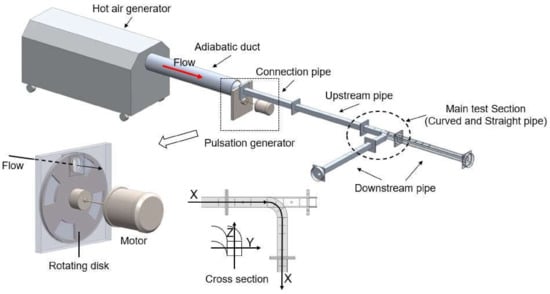
Figure 1.
Diagrammatic sketch of experimental apparatus and coordinate system.
Schematic diagrams of the test pipes are shown in Figure 2. The pipes were made of aluminum, and the processed inner and outer diameters of the pipes were 32 and 40 mm, respectively. According to [18], there are not enough temperature measuring points in the area formed by secondary flow to capture the detailed temperature distribution. In the present study, the number of measurement holes was increased to 126. Among these holes, 120 holes with a diameter of 1.6 mm were drilled on the top surface of the pipes for the K-type thermocouple (T34, Okazaki, Kobe, Japan) insertion to measure the air temperature, and six holes with a diameter of 8 mm were drilled for another type of K-type thermocouple (T32, Okazaki, Kobe, Japan) insertion to measure the temperature oscillation under pulsating flow. As shown in Figure 3b, the T32 K-type thermocouple is composed of a 13 μm thermocouple and a 25 μm thermocouple. Two holes with a diameter of 5 mm were drilled on the bottom surfaces of the upstream and downstream pipes, respectively. A hot-wire anemometer (0251R-T5, Kanomax, Andover, NJ, USA) was installed in these two holes to measure the inlet and outlet velocities of the hot air after calibration with a pitot tube under the high temperature. Figure 3a,b shows the methods used to measure the velocity and temperature, respectively. The temperature field and velocity are measured separately as in Figure 3a. The temperature field was measured after the velocity condition had been measured, so the influence of the size of the hot wire on the temperature field measurement of the test part can be ignored. The temperature fields of corresponding cross-sections as shown in Figure 2 were measured one by one, and the temperatures of the 36 points in each cross-section as shown in Figure 3c were measured point by point. Therefore, the influence of the size of the T34 K-type thermocouple on the measurement results can be ignored. Although the T32 K-type thermocouple as shown in Figure 3b is relatively large, it will affect the downstream flow field and temperature distribution. Thus, we measured the temperatures of corresponding cross-sections one by one. When a hole in Figure 3b is inserted by the thermocouple, the other holes are filled with screws to reduce the measurement error.
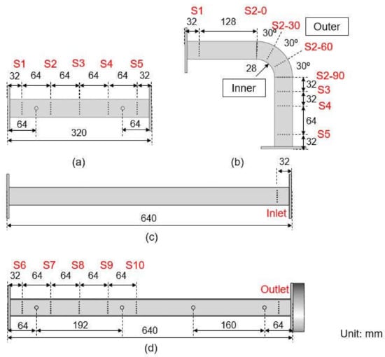
Figure 2.
Diagrammatic sketch of measurement points on pipes (top view): (a) straight pipe; (b) curved pipe; (c) upstream pipe; (d) downstream pipe [18].
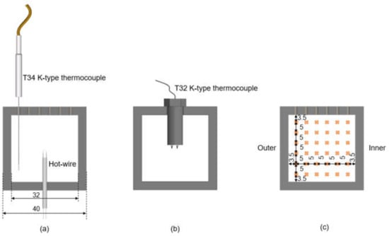
Figure 3.
Cross-section of pipes (from upstream view): (a,b) measurement methods; (c) measurement points [18].
T34 K-type thermocouples were used to measure the hot air time-averaged temperature of each cross-section. As shown in Figure 3c, each section comprised 36 temperature measurement points. The straight and curved pipes have 12 and 15 temperature measurement cross-sections, respectively. T32 K-type thermocouples were used to measure the hot air temperature oscillations under pulsating flow.
As shown in Figure 2, to facilitate the subsequent discussion, the first measurement section named “Inlet” at the outlet of the upstream pipe is defined as the origin. S1 to S10 represent the ten measured cross-sections in the straight pipe. The four sections of the 90° curved part in the curved pipe were numbered as S3-0, S3-30, S3-60, and S3-90. The remaining cross-sections were numbered S1, S2, and S4–S10. The outlet of the downstream pipe was set as the “Outlet” section.
To examine the inflow conditions of steady and pulsating flows at the “Inlet” section, as shown in Figure 4, the time history of the streamwise velocity of both steady flow and pulsating flow was measured using a hot-wire anemometer. The sampling frequency was 10,000 Hz, and the frequency of the pulsating flow was 30 Hz. The time-averaged velocities of the steady and pulsating flows were almost the same.
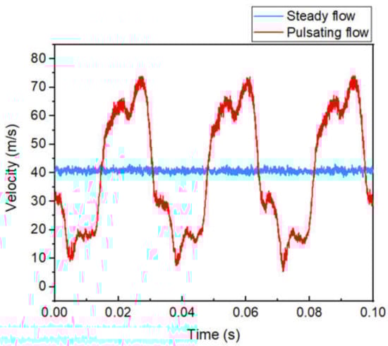
Figure 4.
Instantaneous velocities at the “Inlet” section of the steady flow and pulsating flow.
2.2. Data Processing
Owing to the insufficient dynamic properties of the temperature sensor and the interpretation of recorded signals, which are composed of static and dynamic temperatures, the fluid temperature in pulsating flow is one of the most difficult and complex flow parameters to be measured [25]. A reliable technique studied by Tagawa et al. [26] for estimating thermocouple time constants without any dynamic calibration was applied in the present study to estimate the real hot air temperature of the pulsating flow.
The first-order lag systems of the two thermocouples were used to obtain the fluid temperatures (Tg1 and Tg2) using the following equations:
where T, τ, and G represents the raw temperature, time constant, and derivative of T, respectively. The subscripts “1” and “2” represent the thermocouples of 13 μm and 25 μm in diameter, respectively.
The highest similarity between Tg1 and Tg2 by maximizing the correlation coefficient R is as follows:
Equation (2) was used to diminish the effect of the noise and the irrelevant signal.
The time constants to maximize R should satisfy the following condition:
Simultaneously, the above equations can finally obtain the fluid temperatures (Tg1 and Tg2) after calculating the time constants τ1 and τ2. The time constants of the 13 and 25 μm thermocouples are 9.4 and 21.8 ms, respectively.
Figure 5 shows a sample of the comparison of the original temperature measured by the 13 and 25 μm thermocouples and the estimation of these two thermocouples. The measurement position in this sample was at the midpoint of the upstream pipe. The estimated temperatures of these two thermocouples overlapped well, and the amplitudes of these two estimated temperatures were higher than the measured values.
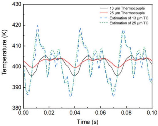
Figure 5.
A sample of the comparison of the original and estimated temperatures.
To calculate the total and local heat transfer in the pipes, the thermophysical properties of hot air to calculate heat transfer were obtained at the mean temperature as follows:
where the subscripts “i” and “o” denote the “Inlet” and “Outlet” sections, respectively. In both the steady flow and the pulsating flow, the spatial average temperature of the Nc = 36 points in the cross-section, as shown in Figure 3c, was used in the calculation. The temperature of each point was the time average of Tmea = 30 s.
The local heat flow rate (Qx) was calculated using the following equation:
where Cp is the constant pressure specific, is the mass flow rate expressed as follows:
where ρ denotes the density of air, Ac denotes the cross-sectional area of the square pipes, and denotes the time average of the velocity. Δx is half the distance between two adjacent cross-sections in the streamwise direction. Tx is the local position temperature, expressed as follows:
where Tnx is the temperature of the nth point in the local cross-section, t is the temperature sampling time.
Finally, the local heat flux (qx) was obtained as follows:
where Aw denotes the pipe wall area of the local section at x. Four rectangular pipe walls are used for the straight pipe. The curved part of the curved pipe is composed of two sectors and two curved surfaces.
Because the total wall areas of the test sections in the straight and curved pipes are different, it is appropriate to use the total heat flux to characterize the heat transfer performance. The total heat flux (qt) was calculated using the following equation:
where Atw denotes the total wall area of the test section, and Qt denotes the total heat flow rate, expressed as follows:
The measurement accuracies of the major parameters used are shown in Table 1.

Table 1.
Major parameter uncertainties [18].
3. Numerical Simulations
Numerical simulations were implemented using CONVERGETM (Convergent Science, Madison, WI, USA). The CHT method was used to solve the flow and heat transfer in both the solid and fluid regions. The computational domain included an upstream pipe, the main test section (curved pipe/straight pipe), and a downstream pipe that was the same as the piping layout in the experiment. A modified cut-cell Cartesian mesh generation method was used for the geometric surface. The computational domain was discretized using cube meshes, and the mesh size was 1 mm. Figure 6 shows the details of the mesh.
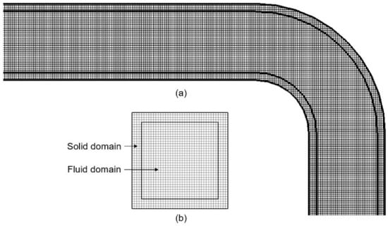
Figure 6.
Computational mesh in the curved pipe. (a) side view, (b) upstream view at the cross-section [18].
In the CHT simulation, the temperature and heat flux of the fluid and solid regions were consistent at the interface. The interface boundary definition is the connecting surface between the fluid and solid regions. For the turbulence model, the RNG k–ε model was applied to calculate the turbulent flows. In addition, the law of the wall was adopted for the velocity calculation on the solid walls to deal with the boundary layer on the wall using the RNG k–ε model. For the temperature law of the wall boundary condition, the Han and Reitz model [27] was used to account for compressible effects in a pulsating flow.
In this study, the Reynolds number is expressed as follows:
where D denotes the hydraulic diameter of the pipe, which is the same as the inner diameter of the pipe, and ν denotes the kinematic viscosity of the fluid.
The Dean number was first proposed by Dean (1959) to characterize curved pipe flows, and it was defined using the following equation:
where Rc denotes the radius of curvature of the curved pipe.
The most commonly used dimensionless parameter to characterize pulsating flow is the Womersley number, which is given by:
where ω is the angular frequency of the pulsation.
The simulation inlet boundary conditions for the velocity and temperature were measured by the hot-wire and the thermocouple separately in the experiment. The outlet pressure boundary condition was set as 101.325 kPa, and the temperature of the reverse flow at the outlet was set at 300 K. A no-slip wall boundary condition was employed on the solid domain side of the interface. The convection boundary condition was adopted on the outer side of the solid domain. The ambient temperature outside the pipe was set as 298.15 K, which is the same as the room temperature in the experiment. The heat transfer coefficient of this convection boundary was selected to be 14 W/m2·K. The heat transfer coefficient of 14 W/m2·K was chosen because previous studies [18] confirmed that the simulation results were in good agreement with the experimental results. For the experimental and numerical conditions, the inlet temperature was set to 402 K. The time-averaged Reynolds number was approximately 60,000 in both the straight and the curved pipes. The Dean number was 31,000 in the curved pipe. The Womersley number was 43.1, in the pulsating flows.
4. Results and Discussion
4.1. Reverse Flow at the Outlet under Pulsating Flow Conditions
Many experimental and numerical studies have shown that reverse flow occurs under pulsating flow conditions, particularly in the large amplitude of the pulsating flow [28,29,30]. As shown in Figure 7, the time history of the streamwise velocity of the pulsating flow at the “Outlet” was measured using a hot-wire anemometer. The signal output of the hot-wire anemometer was a voltage signal, and the velocity value was calculated from the voltage signal through a linear relationship. The green circles in the figure indicate that, during the deceleration of the pulsating flow, the voltage signal changes abruptly. The voltage is a scalar quantity, and the velocity is a vector quantity, thus the velocity flows in the opposite direction during these regions.
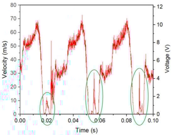
Figure 7.
The voltage signal and the velocity of the pulsating flow at the “Outlet” section.
The velocity experiment results at the “Outlet” verify the existence of reverse flow under the condition of pulsating flow. The reverse flow inhaled the discharged air into the pipe, and the temperature of the air was low. Therefore, the reverse flow phenomenon caused the heat transfer performance at the outlet section to be different from that at the upstream section. The specific effect of reverse flow on heat transfer is discussed in detail later section.
4.2. Circumferential Temperature Fields in the Cross-Sections
For the convenience of description, the steady flow in the straight pipe, the pulsating flow in the straight pipe, the steady flow in the curved pipe, and the pulsating flow in the curved pipe were referred to as “SS”, “PS”, “SC”, and “PC”, respectively. For the circumferential time-averaged temperature fields, color contours of temperature for the experiment were created using MATLAB (MathWorks Inc., Portola Valley, CA, USA) codes based on 36 temperature measured points of each cross-section. The inlet temperature fields of the steady and pulsating flows in the straight and curved pipes are shown in Figure 8. At the “Inlet” section, the temperature field is almost the same under these four experimental conditions. The temperature contours show a nearly concentric circular distribution. In the same pulsation generator device, the stereo particle image velocimetry (PIV) measurement in a double 90° square pipe was studied by Oki [22]. It was reported that because of the rotating disk effect, the velocity distribution 3D upstream of the first curved entrance was point-symmetrical, and the distribution shape was consistent with the temperature distribution shape in the present study.
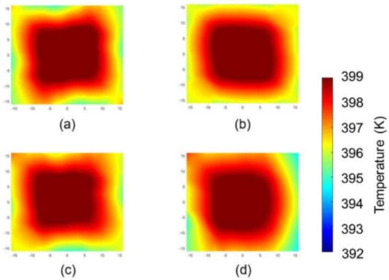
Figure 8.
Temperature contour comparison among the “Inlet” conditions: (a) ”SS”; (b) “PS”; (c) “SC”; (d) ”PC”.
Figure 9 and Figure 10 show the temperature contours of different cross-sections of the “SS” and “PS”, respectively. In the temperature contours from S1 to S10, the temperature gradually decreased. Compared to the “SS”, the temperature drop of the “PS” was less. The temperature in each cross-section decreased from the center to the surroundings. Comparing the central areas of the cross-sections of the “SS” and “PS”, the temperature distribution in the high-temperature core area of the “SS” was concentrated, while that of “PS” was larger.
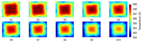
Figure 9.
Temperature contours of different cross-sections of the “SS”.
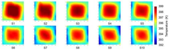
Figure 10.
Temperature contours of different cross-sections of the “PS”.
The temperature contours of the different cross-sections of “SC” and “PC” are shown in Figure 11 and Figure 12, respectively. When compared to the temperature fields in the straight pipe, the temperature fields in the curved part and downstream of the curved part changed significantly. Owing to the influence of the centrifugal force at the curved part (from S2-0 to S3), the high-temperature core gradually shifted to the outer side. In a curved pipe, the typical secondary flow structure is the Dean vortices (two symmetrical counter-rotating vortices). With the generation of the secondary flow, the temperature fields gradually formed a vortex secondary distribution. In downstream of the curved part, this secondary flow distribution gradually weakens along the flow direction. The temperature fields of “SC” and “PC” showed the same changing trend.
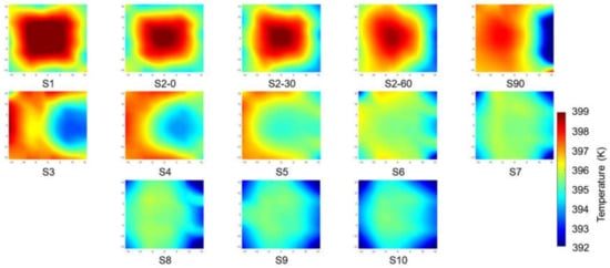
Figure 11.
Temperature contours of different cross-sections of the “SC”.
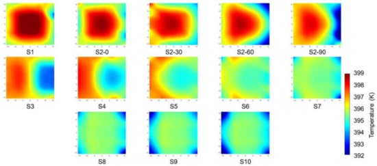
Figure 12.
Temperature contours of different cross-sections of the “SC”.
The temperature near the inner side is particularly low in the S90, which is the exit of the curved part. Combined with previous study [23], this phenomenon was caused by the separation of air and the pipe wall.
Figure 13 shows the temperature fields of the “Outlet” of the “SS”, “PS”, “SC”, and “PC”. As shown in Figure 8, the “Inlet” conditions of the “SS”, “PS”, “SC”, and “PC” were set to be nearly the same. The “Outlet” temperature distribution can directly show the total temperature difference between “Inlet” and “Outlet” under these four conditions. Regardless of the straight pipe or curved pipe, the “Outlet” temperature of the steady flow condition is higher than that of the pulsating flow. However, comparing Figure 9, Figure 10, Figure 11 and Figure 12, the temperature reduction of the steady flow was larger than that of the pulsating flow. Regarding the small temperature reduction of the pulsating flow, the “Outlet” temperature was lower; it was caused by the reverse flow. Reverse flow is the process of returning the air that has been exhausted from the pipe back into the pipe. The exhausted air was mixed with the low-temperature ambient air so that the time average temperature of the pulsating flow at the “Outlet” was lower than that of the steady flow.
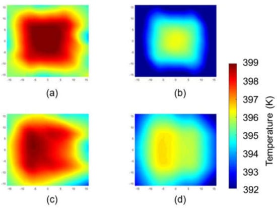
Figure 13.
Temperature contour comparison among the “Outlet” conditions: (a) “SS”; (b) “PS”; (c) “SC”; (d) “PC”.
4.3. Streamwise Temperature Variation
As shown in Figure 14, the average temperature of the cross-sections of the “SS”, “PS”, “SC”, and “PC” decreased as the air flows downstream. The abscissa “X/D” is the streamwise dimensionless length, where D denotes the inner diameter of the pipe. The origin of X/D is defined at the “Inlet”. Figure 14a shows the temperature variation from the “Inlet” to the “Outlet”. In the cases of pulsating flow (“PS” and “PC”), the temperature dropped sharply at the “Outlet” because of the influence of the reverse flow. Figure 14b shows the temperature variation along the streamwise direction from “Inlet” to “S10” after ignoring the effect of reverse flow at the “Outlet”. In the “SS”, the temperature decreased linearly and monotonously along the streamwise direction. In the “PS”, although the temperature showed a decreasing trend, the decline gradually slowed down during the “Inlet” to “S10”. From “S10” to the “Outlet”, the temperature decreased sharply. In the two cases of the curved pipe (“SC” and “PC”), the streamwise temperature variation was more complicated than that of the straight pipe. Regardless of the steady flow or pulsating flow, the temperature exhibited a sharp drop in the curved part. Then, the temperature decline slowed until S10.
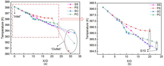
Figure 14.
Average temperatures in the streamwise direction of the “SS”, “PS”, “SC”, and “PC”: (a) all measurement sections, (b) from “Inlet” to S10.
Among these four conditions, regardless of the “Outlet” section, the temperature reduction of the pulsating flow condition is smaller than that of the steady flow. In the case of steady flow, from the “Inlet” to the “Outlet”, the temperature changed smoothly and there was no sudden change from “S10” to the “Outlet”. In the cases of pulsating flow, the temperature dropped sharply at the “Outlet” owing to the effect of the reverse flow.
4.4. Temperature Oscillations in Pulsating Flow
Some studies [5,11,16] have shown that the velocity amplitude of the pulsating flow is a significant factor that affects the heat transfer performance. However, there are a few studies on the investigation of the local temperature amplitude of the pulsating flow. As shown in Figure 2, there are six temperature measurement points (X/D = 3, 9, 13, 19, 24, and 29) along the streamwise direction in the straight pipe. These points were used to insert a T32 K-type thermocouple to measure the center temperature of each cross-section. Figure 15 shows the time history of the air temperature difference from the time average temperature of the different cross-sections of the “PS”. For convenience of comparison, the time average temperature of each cross-section was set to “zero” for all these conditions. The temperature oscillations gradually weakened along the streamwise direction. The closer it is to the pulsation generator, the greater is the amplitude of the temperature. It can be observed from Figure 14 that the greater the amplitude of the temperature, the larger is the temperature decline.
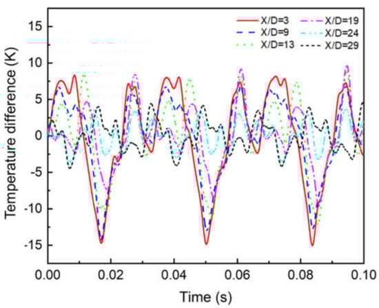
Figure 15.
Temperature difference from the time average temperature of the different cross-sections of the “PS”.
When the velocity amplitude is constant, the local heat transfer performance depends on the amplitude of the temperature. A large temperature amplitude can enhance the heat transfer.
4.5. Heat Transfer Performance Analysis
Heat flux is an important parameter that can reflect heat transfer performance. As shown in Figure 16, the local heat flux at different positions along the streamwise direction intuitively illustrated the heat transfer performance of the “SS”, “PS”, “SC”, and “PC”. The heat flux of the “SS” maintained almost the same value at different positions. At downstream of the straight pipe, the heat flux slightly decreased. The reason for the decrease in heat flux is that in this region, the temperature of the air inside the pipe decreases and the temperature of the pipe wall also decreases, resulting in a smaller temperature difference between the pipe wall and ambient temperatures. According to the thermal boundary condition of the pipe wall in this study, the smaller the temperature difference between the pipe wall and ambient temperatures, the smaller the heat flux is.
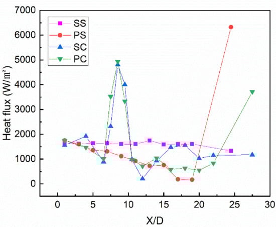
Figure 16.
Heat flux of the different cross-sections of the “SS”, “PS”, “SC”, and “PC”.
The heat flux change trend of the “PS” was quite different from that of the “SS”. The heat flux of “PS” decreased monotonously along the streamwise direction, except at X/D = 25. Under the pulsating flow of the straight pipe, the local heat flux at the entrance of the test section (X/D = 1–3) was higher than that of the straight pipe. In the subsequent sections (X/D = 3–19), the heat flux of the steady flow increased, and the heat flux difference between the steady flow and pulsating flow gradually increased. The heat flux of X/D = 25 increased sharply; however, this does not indicate that the heat transfer was enhanced. As discussed in Section 4.1, there was reverse flow, which made the temperature at the “Outlet” abnormally low.
In the “SC” and “PC”, owing to the impact of the secondary flow and the high-temperature core impingement, the heat flux was maintained at a high level near the outlet of the curved part (X/D = 6–10). At downstream of the curved part (X/D = 10–22), the magnitude of the heat flux was restored to the same level as that of the straight pipe. Similarly, the heat flux of X/D = 25 increased under the pulsating flow condition of the curved pipe because of the reverse flow; however, this does not indicate the enhancement of heat transfer at the location.
If the effect of reverse flow was ignored, the total heat flux from the “Inlet” to “S10” of the steady flow and the pulsating flow in the curved pipe were 8% and 65% higher than that of the straight pipe, respectively. The heat flux of the steady flow in the straight and curved pipes was 64% and 10% higher than that of the pulsating flow, respectively. It is worth noting that at the entrance of the test section, the local heat flux of the pulsating flow is higher than that of the steady flow, and the closer to the pulsation generator, the larger the temperature amplitude is and the higher the local heat flux of the pulsating flow is.
4.6. Numerical Analysis of Heat Transfer Mechanism
To further study the heat transfer mechanism of the pulsating flow, a CHT simulation was used to show more details.
At the beginning of the numerical analysis, both the flow velocity and fluid temperature were validated using the simulation model and simulation setup. In previous studies [18], validation under steady flow conditions was verified. The validation of the temperature oscillation in the pulsating flow is also provided in this study. Figure 17 shows a comparison of the temperature difference from the time-averaged temperature at two different locations (X/D = 3, 29) in the experiment and simulation. For convenience of comparison, the time average temperature was set to “0” for all these conditions. Whether at the “Inlet” (X/D = 3) or “Outlet” (X/D = 29) of the test section, the amplitude of the temperature oscillations can be well-matched. The maximum and minimum temperatures appear simultaneously. Because the frequency derived from the simulation results is much lower than the experimental sampling frequency, there is a slight deviation in the temperature between the experiment and the simulation at some instants. For the validation of the velocity fields, Oki et al. [31] investigated the velocity fields in the curved pipe by PIV measurement. The numerical simulation results proposed by Oki et al. were used to compare with the PIV results of the streamwise velocity distribution at the exit of the pipe curved part, and they are in good agreement. The simulation in this study is based on the same numerical method as Oki et al., so it is reliable to be used.
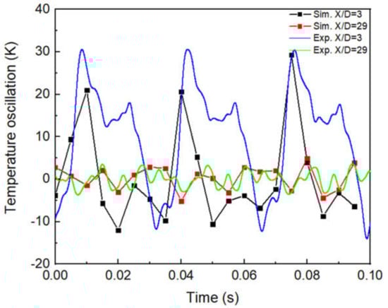
Figure 17.
The experimental and numerical temperature comparison in pulsating flow.
Finally, the simulation results were used to illustrate the heat transfer phenomena that could not be observed in the experiment, and the influence mechanism of pulsating flow on the heat transfer process was explained in detail.
As shown in Figure 18, the instantaneous streamwise velocity vectors and temperature contours of the horizontal section along the center axis in the curved pipe were used to reveal the heat transfer mechanism in the pulsating flow. Figure 18a,b shows the velocity vector and temperature contour of the steady flow at the curved part of the pipe, respectively. They were used for comparison with pulsating flow situations. The velocity vector and temperature contour during the deceleration phase of the pulsating flow is as shown in Figure 18c,d, respectively. The separation between the air and solid wall in the deceleration phase is larger than that in the steady flow. The air temperature was low in the separation region, which reduced the temperature difference between the wall and ambient temperatures. Thus, the heat flux was reduced in this region. The large separation in the deceleration resulted in the suppression of heat transfer downstream of the curved part.
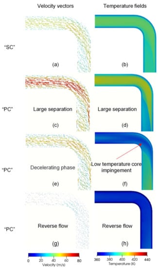
Figure 18.
Instantaneous velocity vectors and temperature fields of the horizontal section along the center axis of the curved pipe in the simulation: (a) and (b) are results of the steady flow, (c) and (d) are the results of the deceleration phase of the pulsating flow, (e) and (f) are results of the pulsating flow approaching the minimum velocity, (g,h) are results of the reverse flow.
For a steady flow in a curved pipe, the impingement of the high-temperature core can enhance the heat transfer, as shown in Figure 18b. However, for the pulsating flow, the temperature changed periodically. Owing to the compressibility of air, a high-temperature air region appeared in the acceleration phase, and a low-temperature air region appeared in the deceleration phase. Figure 18e,f shows the velocity vector and temperature contour, respectively, during the deceleration phase of the pulsating flow before the minimum velocity. The flow impingement phenomenon of the low-temperature core reduced the outer wall temperature of the curved part of the pipe. The temperature difference between the outer wall and ambient temperatures was reduced, and the heat transfer was suppressed in this region. Figure 18g,h shows the temperature and velocity contours of the reverse flow downstream of the curved pipe, respectively. Because the temperature of the reverse flow was low, the wall temperature was reduced sharply during the period when the reverse flow occurred. Therefore, the heat flux decreases in the region where there is a reverse flow. In general, the large separation, impingement of the low-temperature core, and reverse flow were all behaviors of heat transfer suppression.
5. Conclusions
In this study, experiment and simulation of turbulent steady and pulsating flows were performed for straight and 90° curved square pipes. The velocity measurement at the “Outlet” verified the existence of reverse flow under a pulsating flow with a large velocity amplitude. In both the streamwise and circumferential directions, the results of temperature fields in the experiment reported the difference between the steady and pulsating flows in the straight and curved pipes. For the straight pipe, the average cross-section temperature of the steady flow decreased linearly and monotonically in the streamwise direction. The streamwise temperature of the pulsating flow decreased nonlinearly. For both the steady and pulsating flows in the 90° curved pipe, the temperature decreased significantly near the outlet of the curved part of the pipe. The secondary temperature distribution is formed with the formation of Dean vortices.
The local heat flux of different cross-sections in the experiment provided quantitative results of the heat transfer. The local heat flux of the pulsating flow in a straight pipe exhibits a large variation in different cross-sections. The closer to the pulsation generator, the larger the temperature oscillation and the higher the heat transfer performance are. It has an extremely large local heat flux near the outlet of the curved part of the curved pipe. In the test section, for both the steady and pulsating flows, the total heat flux of the curved pipe was higher than that of the straight pipe. For both straight and curved pipes, the total heat flux of the steady flow was higher than that of the pulsating flow.
The instantaneous velocity and temperature fields of the numerical simulation were employed to illustrate the heat transfer mechanism of the pulsating flow. The behaviors, such as the large separation between the air and pipe wall, impingement of the low-temperature core, and reverse flow, suppressed the heat transfer. The conclusions on the phenomena of pulsating flow can be used as a reference in the design and optimization of intake and exhaust manifolds.
Author Contributions
Conceptualization, K.N., H.H., M.K. (Masanobu Koutoku), R.Y., H.Y. and S.S.; methodology, G.G., Y.O., M.K. (Masaya Kamigaki) and Y.I.; software, G.G.; validation, G.G.; formal analysis, G.G. and M.K. (Masaya Kamigaki); investigation, G.G., M.K. (Masaya Kamigaki), and Y.I.; resources, H.H.; data curation, G.G.; writing—original draft preparation, G.G.; writing—review and editing, Y.O.; visualization, G.G.; supervision, K.N. and Y.O.; project administration, H.H.; funding acquisition, H.H. All authors have read and agreed to the published version of the manuscript.
Funding
This research received no external funding.
Institutional Review Board Statement
Not applicable.
Informed Consent Statement
Not applicable.
Data Availability Statement
The data presented in this study are available on request from the corresponding author. The data are not publicly available due to huge experiment and simulation results and the complexity of the data analysis process.
Acknowledgments
Thanks to the Hoday from Editage Group (www.editage.com 25 May 2021) for editing a draft of this manuscript. This research did not receive any specific grant from funding agencies in the public, commercial, or not-for-profit sectors.
Conflicts of Interest
The authors declare no conflict of interest.
Nomenclature
| A | surface area [m2] |
| Cp | constant pressure specific [J/kg·K] |
| D | pipe inner diameter [mm] |
| De | Dean number |
| G | derivative of temperature [K/s] |
| m | flow mass [kg] |
| N | total points of each cross section |
| Q | heat flow rate [W] |
| q | heat flux [W/m2] |
| R | correlation coefficient |
| Re | Reynolds number |
| Rc | radius of curvature [mm] |
| T | temperature [K] |
| Tmea | Temperature measurement time [s] |
| t | time [s] |
| U | velocity [m/s] |
| X | streamwise coordinate |
| Y | horizontal coordinate |
| Z | vertical coordinate |
| Greek Symbols | |
| λ | heat conductivity [W/m·K] |
| ρ | density [kg/m3] |
| ν | kinematic viscosity [m2/s] |
| α | Womersley number |
| ω | angular frequency [rad/s] |
| τ | time constant of thermocouple |
| Subscripts | |
| 1 | thermocouple of 13 μm |
| 2 | thermocouple of 25 μm |
| c | cross section |
| i | inlet |
| g | fluid |
| n | nth point |
| o | outlet |
| t | total |
| w | wall |
| x | local position |
| Superscripts | |
| ¯ | time average value |
| ˙ | rate |
References
- Host, R.; Moilanen, P.; Fried, M.; Bogi, B. Exhaust System Thermal Management: A Process to Optimize Exhaust Enthalpy for Cold Start Emissions Reduction; SAE Technical Paper; SAE International: Warrendale, PA, USA, 2017. [Google Scholar]
- Zhao, T.S.; Cheng, P. Oscillatory Heat Transfer in a Pipe Subjected to a Laminar Reciprocating Flow. J. Heat Transf. 1996, 118, 592–597. [Google Scholar] [CrossRef]
- Habib, M.A.; Attya, A.M.; Eid, A.I.; Aly, A.Z. Convective heat transfer characteristics of laminar pulsating pipe air flow. Heat Mass Transf. 2002, 38, 221–232. [Google Scholar] [CrossRef]
- Yu, J.-C.; Li, Z.-X.; Zhao, T.S. An analytical study of pulsating laminar heat convection in a circular tube with constant heat flux. Int. J. Heat Mass Transf. 2004, 47, 5297–5301. [Google Scholar] [CrossRef]
- Guo, Z.; Sung, H.J. Analysis of the Nusselt number in pulsating pipe flow. Int. J. Heat Mass Transf. 1997, 40, 2486–2489. [Google Scholar] [CrossRef]
- Hsiao, K.-L. Micropolar nanofluid flow with MHD and viscous dissipation effects towards a stretching sheet with multimedia feature. Int. J. Heat Mass Transf. 2017, 112, 983–990. [Google Scholar] [CrossRef]
- Wang, X.; Zhang, N. Numerical analysis of heat transfer in pulsating turbulent flow in a pipe. Int. J. Heat Mass Transf. 2005, 48, 3957–3970. [Google Scholar] [CrossRef]
- Elshafei, E.A.M.; Safwat Mohamed, M.; Mansour, H.; Sakr, M. Experimental study of heat transfer in pulsating turbulent flow in a pipe. Int. J. Heat Fluid Flow 2008, 29, 1029–1038. [Google Scholar] [CrossRef]
- Bouvier, P.; Stouffs, P.; Bardon, J.-P. Experimental study of heat transfer in oscillating flow. Int. J. Heat Mass Transf. 2005, 48, 2473–2482. [Google Scholar] [CrossRef]
- Patel, J.T.; Attal, M.H. An experimental investigation of heat transfer characteristics of pulsating flow in pipe. Int. J. Curr. Eng. Technol. 2016, 6, 1515–1521. [Google Scholar]
- Wantha, C. Effect and heat transfer correlations of finned tube heat exchanger under unsteady pulsating flows. Int. J. Heat Mass Transf. 2016, 99, 141–148. [Google Scholar] [CrossRef]
- Nishandar, S.V.; Yadav, R.H. Experimental investigation of heat transfer characteristics of pulsating turbulent flow in a pipe. Int. Res. J. Eng. Technol. 2015, 2, 487–492. [Google Scholar]
- Khosravi-Bizhaem, H.; Abbassi, A.; Zivari Ravan, A. Heat transfer enhancement and pressure drop by pulsating flow through helically coiled tube: An experimental study. Appl. Therm. Eng. 2019, 160, 114012. [Google Scholar] [CrossRef]
- Shiibara, N.; Nakamura, H.; Yamada, S. Unsteady characteristics of turbulent heat transfer in a circular pipe upon sudden acceleration and deceleration of flow. Int. J. Heat Mass Transf. 2017, 113, 490–501. [Google Scholar] [CrossRef]
- Plotnikov, L.V.; Zhilkin, B.P. Specific aspects of the thermal and mechanic characteristics of pulsating gas flows in the intake system of a piston engine with a turbocharger system. Appl. Therm. Eng. 2019, 160, 114123. [Google Scholar] [CrossRef]
- Simonetti, M.; Caillol, C.; Higelin, P.; Dumand, C.; Revol, E. Experimental Investigation and 1D Analytical Approach on Convective Heat Transfers in Engine Exhaust-Type Turbulent Pulsating Flows. Appl. Therm. Eng. 2019, 165, 114548. [Google Scholar] [CrossRef]
- Naphon, P.; Wongwises, S. A review of flow and heat transfer characteristics in curved tubes. Renew. Sustain. Energy Rev. 2006, 10, 463–490. [Google Scholar] [CrossRef]
- Guo, G.; Kamigaki, M.; Zhang, Q.; Inoue, Y.; Nishida, K.; Hongou, H.; Koutoku, M.; Yamamoto, R.; Yokohata, H.; Sumi, S.; et al. Experimental Study and Conjugate Heat Transfer Simulation of Turbulent Flow in a 90° Curved Square Pipe. Energies 2021, 14, 94. [Google Scholar] [CrossRef]
- Chang, L.-J.; Tarbell, J.M. Numerical simulation of fully developed sinusoidal and pulsatile (physiological) flow in curved tubes. J. Fluid Mech. 1985, 161, 175. [Google Scholar] [CrossRef]
- Sudo, K.; Sumida, M.; Yamane, R. Secondary motion of fully developed oscillatory flow in a curved pipe. J. Fluid Mech. 1992, 237, 189–208. [Google Scholar] [CrossRef]
- Najjari, M.R.; Plesniak, M.W. Evolution of vortical structures in a curved artery model with non-Newtonian blood-analog fluid under pulsatile inflow conditions. Exp. Fluids 2016, 57, 100. [Google Scholar] [CrossRef]
- Oki, J.; Kuga, Y.; Yamamoto, R.; Nakamura, K.; Yokohata, H.; Nishida, K.; Ogata, Y. Unsteady Secondary Motion of Pulsatile Turbulent Flow through a Double 90°-Bend Duct. Flow Turbul. Combust. 2019, 104, 817–833. [Google Scholar] [CrossRef]
- Zhai, M.; Wang, X.; Ge, T.; Zhang, Y.; Dong, P.; Wang, F.; Liu, G.; Huang, Y. Heat transfer in valveless Helmholtz pulse combustor straight and elbow tailpipes. Int. J. Heat Mass Transf. 2015, 91, 1018–1025. [Google Scholar] [CrossRef]
- Xu, Y.; Zhai, M.; Guo, L.; Dong, P.; Chen, J.; Wang, Z. Characteristics of the pulsating flow and heat transfer in an elbow tailpipe of a self-excited Helmholtz pulse combustor. Appl. Therm. Eng. 2016, 108, 567–580. [Google Scholar] [CrossRef]
- Olczyk, A. Problems of unsteady temperature measurements in a pulsating flow of gas. Meas. Sci. Technol. 2008, 19, 055402. [Google Scholar] [CrossRef]
- Tagawa, M.; Shimoji, T.; Ohta, Y. A two-thermocouple probe technique for estimating thermocouple time constants in flows with combustion: In situ parameter identification of a first-order lag system. Rev. Sci. Instrum. 1998, 69, 3370–3378. [Google Scholar] [CrossRef]
- Han, Z.; Reitz, R.D. A temperature wall function formulation for variable density turbulent flows with application to engine convective heat transfer modeling. Int. J. Heat Mass Transf. 1997, 40, 613–625. [Google Scholar] [CrossRef]
- Talbot, L.; Gong, K.O. Pulsatile entrance flow in a curved pipe. J. Fluid Mech. 1983, 127, 1–25. [Google Scholar] [CrossRef]
- Toshihiro, T.; Kouzou, S.; Masaru, S. Pulsating flow in curved pipes 1: Numerical and approximate analysis. Bull. JSME 1984, 27, 2706–2713. [Google Scholar]
- Timité, B.; Castelain, C.; Peerhossaini, H. Pulsatile viscous flow in a curved pipe: Effects of pulsation on the development of secondary flow. Int. J. Heat Fluid Flow 2010, 31, 879–896. [Google Scholar] [CrossRef]
- Oki, J.; Ikeguchi, M.; Ogata, Y.; Nishida, K.; Yamamoto, R.; Nakamura, K.; Yanagida, H.; Yokohata, H. Experimental and numerical investigation of a pulsatile flow field in an S-shaped exhaust pipe of an automotive engine. J. Fluid Sci. Technol. 2017, 12, JFST0014. [Google Scholar] [CrossRef][Green Version]


Publisher’s Note: MDPI stays neutral with regard to jurisdictional claims in published maps and institutional affiliations. |
© 2021 by the authors. Licensee MDPI, Basel, Switzerland. This article is an open access article distributed under the terms and conditions of the Creative Commons Attribution (CC BY) license (https://creativecommons.org/licenses/by/4.0/).