Article

FEHCA: A Fault-Tolerant Energy-Efficient Hierarchical Clustering Algorithm for Wireless Sensor Networks

1
Department of Computer Science and Engineering, Graphic Era Deemed to be University, Dehradun 248002, India
2
Faculty of Science and Technology, Mathematics and Computing, Mount Royal University, Calgary, AB T3E 6K6, Canada
3
School of Computer Science, University of Auckland, Auckland 1010, New Zealand
*
Authors to whom correspondence should be addressed.
Energies 2021, 14(13), 3935; https://doi.org/10.3390/en14133935
Submission received: 25 May 2021 / Revised: 18 June 2021 / Accepted: 24 June 2021 / Published: 2 July 2021

Abstract

:
Technological advancements have led to increased confidence in the design of large-scale wireless networks that comprise small energy constraint devices. Despite the boost in technological advancements, energy dissipation and fault tolerance are amongst the key deciding factors while designing and deploying wireless sensor networks. This paper proposes a Fault-tolerant Energy-efficient Hierarchical Clustering Algorithm (FEHCA) for wireless sensor networks (WSNs), which demonstrates energy-efficient clustering and fault-tolerant operation of cluster heads (CHs). It treats CHs as no special node but equally prone to faults as normal sensing nodes of the cluster. The proposed scheme addresses some of the limitations of prominent hierarchical clustering algorithms, such as the randomized election of the cluster heads after each round, which results in significant energy dissipation; non-consideration of the residual energy of the sensing nodes while selecting cluster heads, etc. It utilizes the capability of vector quantization to partition the deployed sensors into an optimal number of clusters and ensures that almost the entire area to be monitored is alive for most of the network’s lifetime. This supports better decision-making compared to decisions made on the basis of limited area sensing data after a few rounds of communication. The scheme is implemented for both friendly as well as hostile deployments. The simulation results are encouraging and validate the proposed algorithm.

1. Introduction

The world is witnessing the increasing involvement of sensors in human life due to the technological advancements that have been achieved in recent decades. Various arrangements of sensors are serving humankind in the present scenario. Wireless sensor networks can be visualised as various sensing nodes sensing a specified domain, gathering information normally pertaining to environmental changes (movement of human beings, animals or vehicles; temperature changes, etc.) and forwarding it to a central control station, generally referred to as a sink or base station (BS), for decision-making purposes [1,2,3].
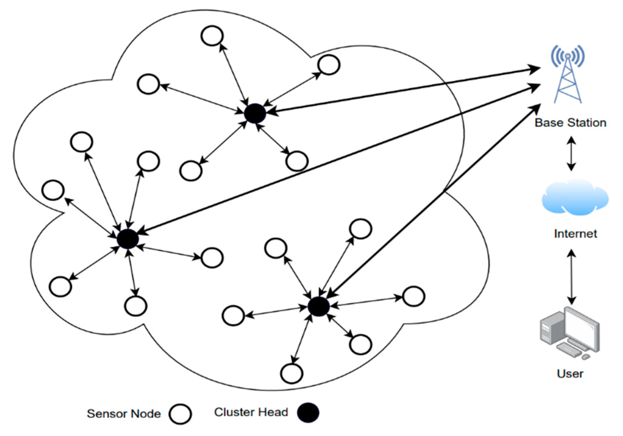
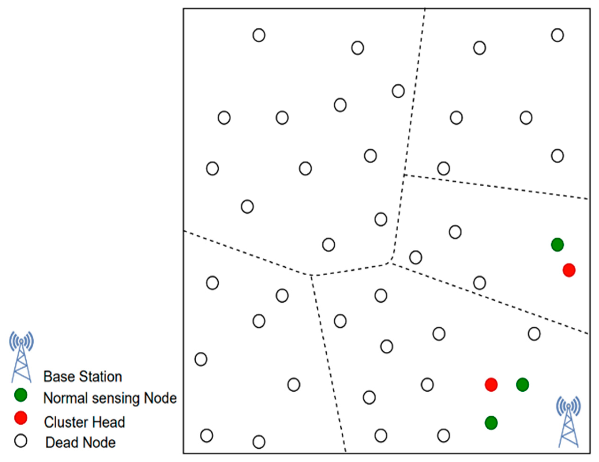
Figure 1 shows a typical hierarchical architecture, where sensing nodes collect the data from the environment and forward it to a leader node in the cluster, referred to as a cluster head (CH), which, after aggregation, further forwards it towards the base station. The analysis of data for decision-making purposes is generally performed at the BS level, but some basic computations can also be performed at the CH level or even at the normal sensing node level depending on the approach used [1,4].
Inherent to the wireless networks are a few constraints such as limited battery life, bandwidth, memory, processing capabilities, abrupt sensor breakdown or abrupt behaviour, etc., which all need to be efficiently addressed. These networks may be deployed in friendly environments such as homes and offices or may be air-dropped into hostile environments where sometimes it is not possible to replace the batteries of the sensors or calibrate the sensors [1,3]. The sensing nodes of WSNs are generally fixed but they may have limited mobility as well, such as sensors floating on water bodies.
Continuing advancements in micro-electro-mechanical systems (MEMS) technology have made it possible to fabricate smaller, inexpensive, energy-efficient sensors with increased memory and increased computational capability [1,5,6,7] (e.g., Mica motes from Crossbow, Tmote Sky from Moteiv, the MKII nodes from UCLA and SunSpot from Sun), which have further boosted confidence in the use of WSNs. The integration of sensing capabilities, computation and communication into a single unit has also been much refined. This has tempted researchers to analyse the sensors’ data for the purpose of efficient decision-making.
Various methodologies have been adopted in relation to WSNs; of late, many researchers have been tempted to use machine learning (ML) in the context of WSNs [8,9]. It provides generalised solutions through an architecture that can learn and improve its performance. The application of ML has led to great improvements in the performance of WSNs. Thus, advancements in machine learning have and are being applied to solve various WSN issues [10,11].
Routing strategies also play a key role in the efficient working of WSNs. These strategies in WSNs, on the basis of the network structure, are broadly classified into flat network routing, location-based routing and hierarchical network routing. In flat network routing, all the sensors are uniformly deployed at the same level and each sensor serves as the other’s peer. This can further be divided into proactive or reactive routing [12]. On the other hand, in the case of location-based routing, the sensors are clustered based on their location in the deployment, which is determined by the received signal strength [13,14].
Amongst the three, hierarchical routing protocols have attracted the attention of many researchers as they ensure better energy efficiency [15,16]. Here, the protocols arrange the deployed sensors into groups and each group has a designated cluster head (generally the sensor with the maximum energy). The cluster head coordinates with all the nodes inside the group, generally called a cluster, and with the activities outside the cluster, whether communicating with other CHs or the BS.
One of the most prominent hierarchical routing protocols is Low-Energy Adaptive Clustering Hierarchy (LEACH). It has shown great energy efficiency and is the basis of various other subsequent routing protocols [17]. It makes use of randomisation for the purpose of evenly distributing the energy load across all the sensing nodes and arranges various sensors into groups, where each group has a special sensor behaving as the leader of the group, coordinating the activities of the group. Here, a few sensors designate themselves as cluster heads based on a certain probability and the number of times they have been the cluster head so far. This leader’s role is rotated so that it does not drain any single sensor’s energy [15].
Since, the deployed battery-operated sensing nodes are energy-constrained, it is important to utilize the energy wisely to extend the network’s lifetime. Moreover, the nodes deployed in hostile environments are very prone to faults, which may be related to a harsh environment, energy depletion or hardware failure. Although it is quite evident that a non-CH faulty node will degrade the network performance, a faulty CH node can be much more problematic, as it will hamper the whole data aggregation and dissemination process of this cluster and will make normal working nodes useless. This paper discusses the basic concept of the hierarchical clustering protocols and proposes a base-station-controlled Fault-tolerant Energy-efficient Hierarchical Clustering Algorithm (FEHCA), which focuses on:
  • The issue of energy efficient clustering to enhance the network lifetime;
  • The optimal cluster counts for the network;
  • The use of k-means clustering that partitions N-nodes into k-clusters, in which each node is associated with the cluster with the nearest mean;
  • The election of CHs near the centroids of the respective clusters for effective inter-cluster communication;
  • Minimization of energy dissipation by deferring the re-election of new CHs after each round;
  • Attempting to make the cluster heads (CHs) fault-tolerant by appointing a secondary cluster head (sCH) in case the current cluster head goes down between two successive rounds.
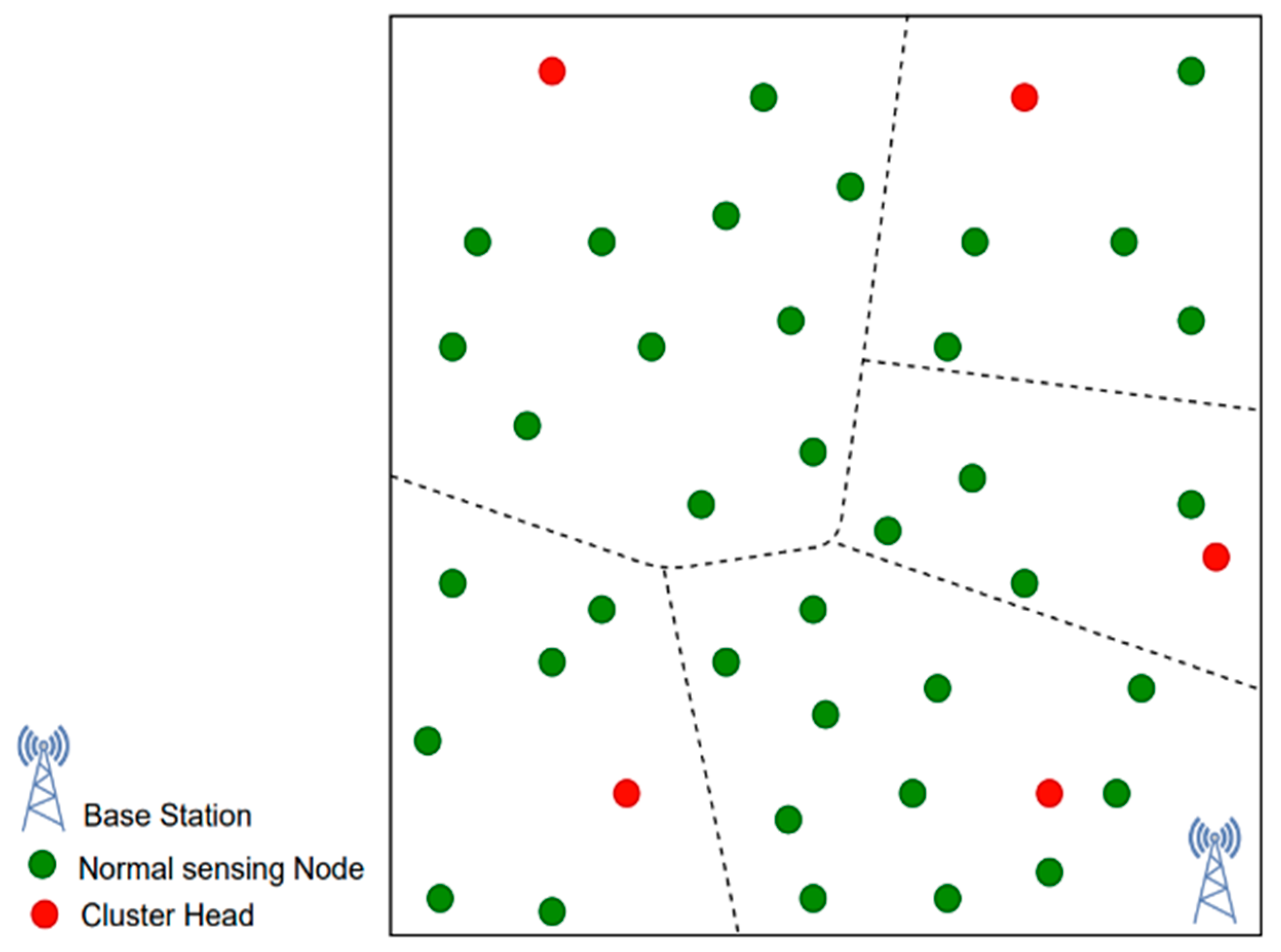
In essence, this paper proposes a centralised cluster formation technique controlled by the base station (BS), where the deployed sensors are divided into an optimal number of clusters. Once the number of clusters is decided and cluster formation is done, the algorithm, instead of electing any arbitrary CH, as shown in Figure 2, elects the CH near the centroid of respective clusters. The algorithm has been developed to be fault-tolerant in the context of the CH and does not require re-cluster formation between two successive rounds if the CH is found to be permanently defective.
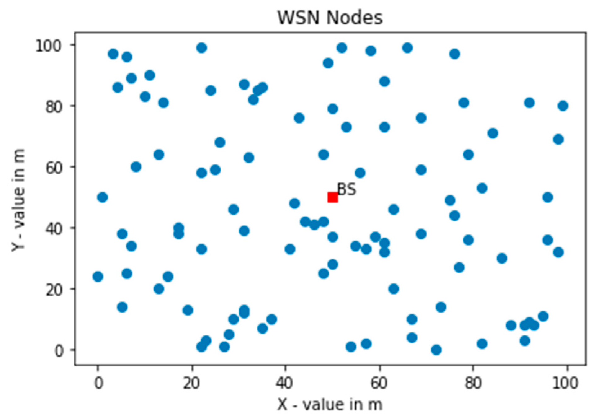
The work was carried out by considering both friendly and hostile environments; thus, the placement of the BS was assumed to be within the deployment and far away from the hostile environment, respectively. The performance of the network highly depends on the placement of the base station. Suppose that a BS is placed within the monitored area (user-friendly environments such homes and offices, etc.); it will be in close proximity to the cluster heads, as compared to a base station, which is outside the monitored area (generally in the case of hostile deployments such as harsh terrains, border areas, etc.), where most of the cluster heads generally will be at a distance from the base station.
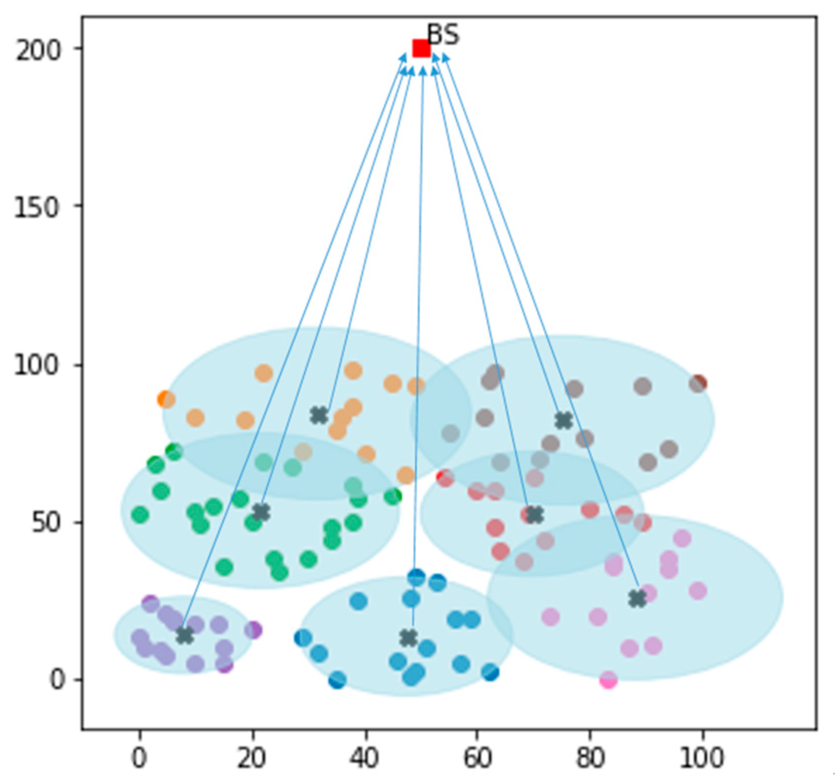
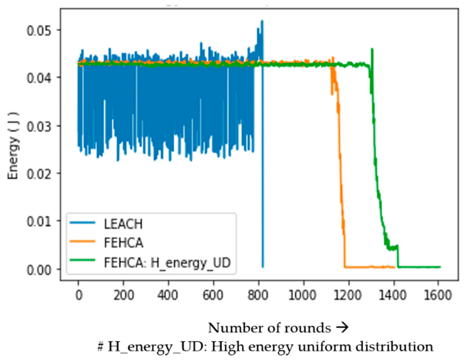
Most of the implementations discuss either friendly environment deployments or hostile environment deployments, but the proposed algorithm was simulated and validated for both scenarios. We also compared our work with some of the state-of-the-art existing technologies with common parameters by positioning the BS within the monitored area. Furthermore, the paper simulates the proposed algorithm in hostile environments by integrating high energy nodes into the network, with the primary aim of keeping the entire monitored area alive for the majority of the lifetime of the network rather than monitoring only the surrounding region after certain rounds of communication, as shown in Figure 3, and the results are promising.
The rest of the paper is organized as follows. Section 2 presents a summary of the related work done in this domain, whereas the proposed system model is explained in Section 3, which includes the network model and energy model for the proposed system. Section 4 discusses the proposed algorithm for cluster head selection and fault tolerance. Investigational outcomes are discussed in detail in Section 5, which also contains the comparative study of our algorithm. Finally, the summary and conclusions are presented in Section 6.

2. Related Work

Clustering and fault tolerance are the focus of various researchers working on wireless senor networks [3,18]. Clustering is generally studied as either centralised or distributed [18]. Centralised clustering involves clustering that is dictated by the base station and the decisions are communicated in the field to the elected CHs; it is generally used in location-aware sensor networks. On the other hand, distributed clustering can be utilised in the case of location-unaware sensor networks, where the sensors are not aware of their relative positioning in the network.
Various hierarchical routing protocols for WSNs have also been presented in the past [15,19,20,21,22]. Heinzelman et al. [
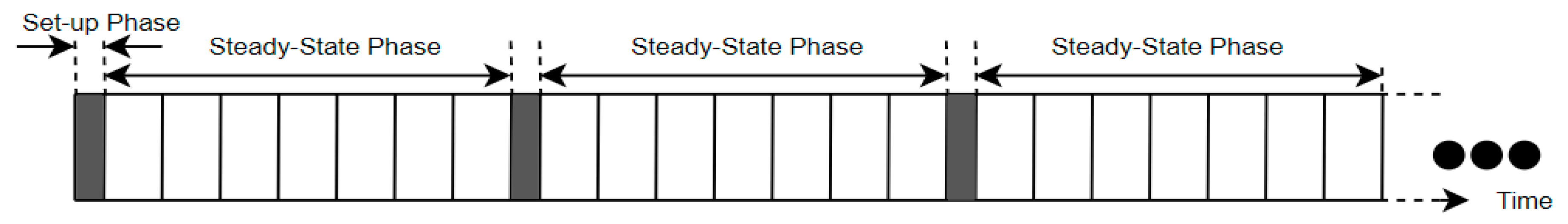
15] presented a two-phase (setup phase and steady phase) cluster-based protocol for WSNs, known as Low Energy Adaptive Clustering Hierarchy (LEACH). Though LEACH was one of the earliest clustering protocols and formed the basis for various forthcoming protocols, it has its own share of shortcomings, which have been addressed by various researchers [23,24,25,26,27,28,29].
Mechta et al. [30] have proposed a protocol named LEACH-CKM that makes use of k-means classification for grouping the nodes. The proposed protocol is based on Centralised LEACH, where CHs are appointed centrally with the help of the CH’s and sensing node’s local information. LEACH-CKM addresses the node isolation problem where a remote node is not able to communicate with the base station. It utilises a Minimum Transmission Energy routing algorithm for routing the information from remote nodes.
An energy-efficient, fault-tolerant, distributed clustering and routing scheme for wireless sensor networks has been proposed by Azharuddin et al. [31]. The proposed scheme is a set of two algorithms jointly named Distributed Fault-tolerant Clustering and Routing (DFCR). It makes use of a distributed run time recovery strategy for the sensor nodes in case of unexpected failure of the cluster heads. The scheme is shown to be capable of handling the sensor nodes that do not have any cluster head to be associated with.
In another work, LEACH’s threshold formula has been modified and presented by Xingguo L et al. [20], where the residual energy is taken into account while selecting a cluster head, as the traditional LEACH does not pay attention to the residual energy of the nodes while choosing the cluster heads, which might lead to a low energy sensor node being elected as the cluster head, which will exhaust early, leading to wastage of resources utilised for cluster head selection. The protocol uses direct BS and CH communication.
Bhatti et al. [32] have proposed a clustering technique using fuzzy c-means. The paper presents a cluster-based cooperative spectrum sensing scheme to reduce energy consumption and proposes an algorithm that creates clusters and elects the cluster heads in such a way that focuses on both the issues of energy consumption and efficiency in a positive manner. The proposed scheme ensures maximum probability of detection under an imperfect channel, utilising minimal consumption of energy when compared with the conventional clustering approaches.
Further, the role of energy balancing in extending the network lifespan has been explored by Azharuddin et al. [33]. The authors propose a Particle Swarm Optimization (PSO)-based routing and clustering algorithm for wireless sensor networks, where the routing algorithm creates a balance between energy efficiency and energy balancing. The clustering algorithm is responsible for the CH and normal sensing node’s energy consumption. The proposed algorithms are also sophisticated enough to handle the failure of cluster heads.
A comparison between Particle Swarm Optimisation and Genetic Algorithm when applied to wireless sensor networks for network optimisation has been presented by Parwekar et al. [34]. It shows how both the algorithms can optimise cluster formation. Their experimental results found that PSO outperformed GA for clustering purposes.
Saveros et al. [35] have proposed a low-power handover design algorithm for wireless sensor networks (WSNs). The algorithm is designed to place the majority of the scanning responsibility on the mains-powered access points. The proposed algorithm has been implemented and empirically evaluated. The evaluation results show that the energy consumption can be reduced by several orders of magnitude compared to existing algorithms for WSNs.
Nigam, G.K et al. [36] have pointed out at some of the drawbacks of the LEACH protocol, such as the unnecessary cluster head election after each round, which results in significant energy depletion, discarding the remaining energy of the sensors, non-uniformity of number of cluster heads, etc. The paper proposes an algorithm, namely ESO-LEACH, for addressing some of these issues. It makes use of metaheuristic particle swarm enhancement for the initial clustering of the nodes, introduces the concept of advanced nodes and also takes the residual energy of the nodes into consideration. An enhanced set of rules and a fitness function are also defined for the purpose of cluster head selection. The algorithm demonstrates enhanced network lifetime as compared to conventional LEACH.
Based on the above observations, it seems that there is a need for a centrally administered fault-tolerant and energy-efficient clustering algorithm. In order to achieve this, we have proposed an improved, centrally administered, fault-tolerant and energy-efficient clustering algorithm that is capable of enhancing the energy load balance and able to achieve encouraging results. Therefore, in the next section, a system model is considered for implementing the proposed algorithm.

3. System Model

A system model has prime importance when it comes to algorithm discussions. In this section, the system model considered in the proposed algorithm is discussed in terms of network model, energy model and fault model.

3.1. Network Model

The proposed work assumes the random deployment of N-sensing nodes that, once deployed, are stationary. The deployed nodes are homogeneous in nature, with identical initial energy and hardware. The basic working principle is divided into rounds as in [37], where each round comprises local data gathering by the sensing nodes, which is forwarded to the cluster head of the particular clusters. On receiving the data, the cluster head aggregates the received data, removes the redundancies and transmits these data to the base station (BS). In between the successive rounds, the nodes are assumed to switch off their radios in order to conserve their batteries. The following assumptions have been considered for this purpose:
Assumption 1.
All the sensing nodes, once deployed, and the base station are stationary.
Assumption 2a.
All the sensing nodes start with the same initial energy (in the case of BS positioned at the centre of the deployment).
Assumption 2b.
The deployment is equipped with advanced nodes in incremental fashion with increasing distance from the BS as per Lemma 2 (in the case of BS positioned outside the deployment area).
Assumption 3.
The BS controls the clustering process and has high computational power and is also not energy-constrained.
Assumption 4.
The BS is within the direct communication range of all the nodes and thus the elected CHs (which communicate directly with the BS).
Assumption 5.
The sensing nodes sense the region at a fixed rate and then communicate the sensed data to the respective CHs.
Assumption 6.
The sensors can adjust the transmission power as the distance to the target changes.
Assumption 7.
The sensors are homogeneous in nature and energy-constrained.
The above-listed assumptions are taken into consideration in order to study the performance of the proposed scheme in line with the other popular schemes mentioned in the paper and highlight the improvements of the proposed scheme in terms of the common parameters.

3.2. Energy Model

The proposed work makes use of the popular energy model described in [37], which makes use of both the free space (d2 power loss) and the multipath propagation (d4 power loss) model depending on the distance between the communicating entities.
If the distance between the sender and the receiver is less than a threshold do, then the free space model is utilised; otherwise, the multipath model is utilised. If Eelec is the amount of energy dissipated by the radio to run the transmitter or receiver circuitry per bit, εfs and εmp are the energy required for amplification in the free space and multipath model, respectively. The energy required by the radio to transmit a k-bit message over a distance d is given by Equation (1) as:
E T x ( k , d ) = { k E e l e c + k ε f s d 2 ,             d < d o   k E e l e c + k ε m p d 4 ,           d d o
To receive the k-bit message, the radio expends E R x energy, as given by Equation (2).
E R x ( k ) = k   E e l e c
The given parameter Eelec depends on numerous factors, such as digital coding, modulation, filtering and spreading of the signal, while the amplification energy εfs and εmp is subject to the distance between the sender and the receiver and to the acceptable bit rate error.
For simulation purposes, the parameters are set to: Eelec = 50 nj/bit, εfs = 10 pj/bit/m2, εmp = 0.0013pj/bit/m4 and EDA = 5 nj/bit/signal. Threshold do is calculated as d 0 = ε f s ε m p .

3.3. Fault Model

Failures are an inherent part of WSNs; different types of faults may affect them [38]. If, in between the CH selection rounds, the CH goes down, then either the data aggregated of that cluster will be lost or a new CH selection will be initiated immediately. The proposed Fault-tolerant Energy-efficient Hierarchical Clustering Algorithm (FEHCA) does not introduce immediate CH selection in between two successive rounds as such a practice leads to energy depletion. The CH going down in between two successive rounds is managed by the sCH node of each cluster, which is on standby in every cluster and takes over the task of CH temporarily.
The algorithm ascertains the selection of the CH at the centroid or near the centroid of the clusters. As a random CH selection does not present an ideal scenario, as shown in Figure 2, unpredictable CH selection generally leads to non-uniform energy dissipation in the network, which ultimately reduces the network lifetime due to the rapid energy discharge. Election of the CH near the centroids makes it easily accessible and helps in achieving uniform energy dissipation, and, once the current CH’s energy is depleted beyond a certain threshold, preference is given to the eligible sensors near the previous round’s CH and the defined energy threshold is satisfied.

4. Proposed Algorithm

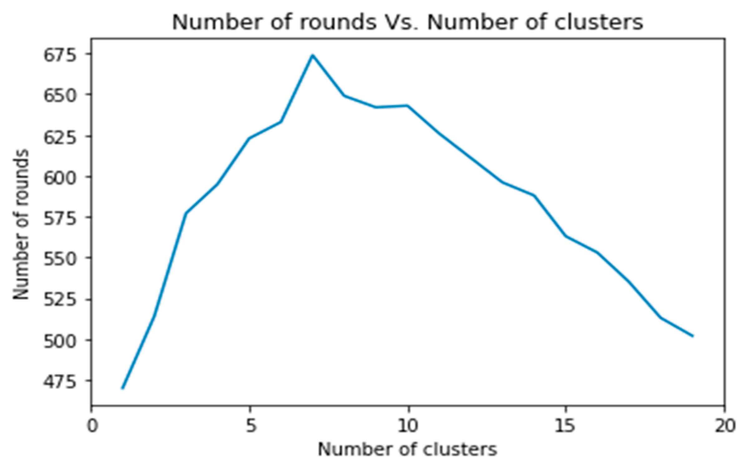
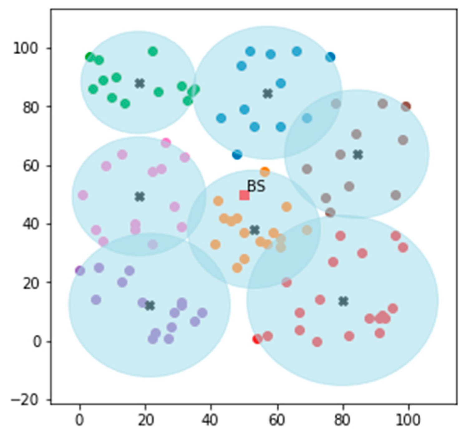
In the proposed algorithm, the network lifetime is divided into several rounds. The algorithm works in two phases, the setup phase and the steady-state phase, as shown in Figure 4. In the setup phase, the base station (BS) gathers the energy and location information of the deployed nodes, based on which it clusters the entire region into an optimal number of clusters (7 optimal clusters in our case), as shown in Figure 5. The BS, after deciding the optimal cluster ratio (Cr) in the network, performs the clustering using the k-means clustering algorithm [39]. Once the clusters are determined, the BS elects the CHs at or near the centroid of the clusters, which is followed by the steady-state phase.
In the steady-state phase, when the cluster formation is accomplished, the non-cluster head sensing nodes sense the region and forward the sensed data to the appropriate CHs. The CHs aggregate the data, look for any redundancy and uncorrelated data and send it to the BS in a single hop. For better energy efficiency, the proposed algorithm elects the CHs near the centroid of the cluster and delays the subsequent setup phases, unlike in LEACH, until the residual energy of the current CH ( C H _ E r e s ) >= specified threshold energy ( C l u s t e r _ E a v g ), thus conserving energy, as each setup phase consumes a significant amount of energy in exchanging the control packets required for the cluster formation.
Algorithm 1 describes the proposed scheme, followed by Lemma 1′s analysis of its complexity. The clustering and cluster head selection processes used in the proposed algorithm are discussed in the following section.

4.1. Clustering Phase

The proposed algorithm uses a popular unsupervised vector quantisation k-means algorithm to divide the randomly distributed sensors into clusters and performs iterative computations to optimise the centroids. The algorithm tries to minimise the distance between the sensor nodes within the clusters with the respective centroids. FEHCA implements a centralised approach where the BS performs the task of clustering. The BS elects the sensor node nearest to the centroid with energy greater than or equal to the average cluster energy, i.e., Eres >= Cluster_Eavg. Here, the current CH retains its role until its energy falls below the average energy of the cluster. Moreover, the number of clusters to be formed is not changed unless the ideal number of clusters required changes. In essence, the clustering phase is divided into two phases, namely centralised clustering and cluster head selection.

4.2. Centralised Clustering

In centralised clustering, each ith node is represented by Ni, where i ∈ {1, 2, …, n}, and the base station is represented as N+. Therefore, the overall entities participating are N= {N1, N2, …, Nn, N+}. N+, based on the sensor’s location and residual energy, partitions the network into clusters; for this, the proposed scheme makes use of k-means clustering as shown in Algorithm 2. Once the clustering decision is made, N+ conveys the clustering information to the sensing nodes (Ni). N+ elects the CHs and sends the corresponding CH parameters to Ni. On receiving the values from the BS, each node determines whether it is the CH or a normal participating node in the current round. If any node is not selected as a CH in the current round, then the N+ directly transmits the Ni value corresponding to the CH with which that node needs to associate. The k-means clustering initially performs a random partition of the network into centroid based k-clusters; then, it repeatedly performs the task of minimising the distance between each node and the respective centroid. Ultimately, this process ensures that the sensor nodes within the cluster are in close proximity. This leads to reduced energy dissipation and efficient communication of the CH with the member nodes, as well as supporting efficient monitoring of the cluster.

4.3. Cluster Head Selection

In this process, the BS (N+) elects the CHs based on the distance from the centroid and the specified energy requirements, and it communicates the Ni value corresponding to the selected CH to the participating nodes in the network. If the received Ni value corresponds to the value of the receiving node, then the recipient recognises itself as the CH and creates and broadcasts to its member nodes for the coordination of the data transmission in the specified schedule. Otherwise, if the Ni value does not correspond to the value of the receiving node, then it recognises itself as a normal member node of the cluster, sends a cluster joining request to the CH whose Ni value it has received from N+ and subsequently waits for the schedule to be generated by its CH. Once this process is completed, each member node in the cluster transmits the sensed data and the corresponding residual energy to the respective CH as per the received schedule. Between the subsequent transmission schedule, the sensor switches off the radios to conserve the energy. The CH compares its energy with the average energy of the cluster and communicates this information to the BS. If its energy is greater than or equal to the average energy of the cluster, then it remains the CH; otherwise, the BS elects a new CH by considering the residual energy and the distance from the centroid in the next round. New CHs are elected from the sensors within the current clusters only, and new clusters are created only when the ideal number of clusters to be formed is changed (depending on the Cr). The cluster head election in FEHCA is shown in Algorithm 1 which has a worst-case time complexity of O (Cn2 + Cn CN2 log CN) and is discussed in Lemma 1.
Algorithm 1. Cluster head election in FEHCA.
Input: ( N , E i , n , C r )
N   ( N i ,     i { 1 ,   2 , ,   n } ) alive nodes with co-ordinates ( x i ,   y i )
E : initial energy ( E 1 ,   E 2 , E 3 , , E n )  
n: number of alive nodes
Cr: Optimal cluster ratio
Output: C H
where CH represents cluster heads
Procedure: F E H C A ( N ,   E i ,   C r ,   n )
1: C n = r o u n d ( n C r )
//Number of clusters in the network
2: C e n t r o i d ,   C N   K M E A N S ( N ,   C n ,   n )
//Calculating cluster(s) centroid, and
respective participating members
3: f o r   i = 1     t o   a l l     c e n t r o i d s   i n   C e n t r o i d
//For finding the minimum distance node
in a cluster
4:     C l u s t e r _ E a v g 0
5:     f o r   j = 1   t o   a l l   m e m b e r   n o d e s   i n   C N
//For all nodes in a cluster
6:            C l u s t e r _ E a v g C l u s t e r _ E a v g + E j
7:            d i j d i s t a n c e   b e t w e e n   c e n t r o i d   a n d   c l u s t e r   n o d e
8:     e n d   f o r
9:     C l u s t e r _ E a v g C l u s t e r _ E a v g n u m b e r   o f   n o d e   i n   C N
10:     w h i l e   C H _ E r e s < C l u s t e r _ E a v g
11:     d o
12:             C H min ( d i )
//CH is elected cluster head
13:                 r e m o v e   C H   f r o m   d i
14:         e n d   w h i l e
15: e n d   f o r
Algorithm 2. K-Means algorithm.
Input: ( N , C n , n )
    N   ( N i ,     i { 1 ,   2 , ,   n } )   alive nodes with co-ordinates ( x l ,   y l )
    C n   represents number of clusters in the network
    n is number of alive nodes
Output: C e n t r o i d ,   C N
Procedure:   K M E A N S ( N ,   C n , n )
1: ( s 1 ,   s 2 ,   s 3 , ,   s C n ) S e l e c t   r a n d o m   s e e d   p o i n t s ( N , C n )
  i { 1 ,   2 , ,   n }
2: f o r   k 1   t o   C n
3:   d o   C e n t r o i d k s k
4: e n d   f o r
5: w h i l e   s t o p p i n g   c o n d i t i o n   i s   n o t   m e t
6: d o
7:   f o r   k 1   t o   C n
8:      C N k {   }
9:   e n d   f o r
10:   f o r   m 1   t o   n
11:      j   argmin j ( ( i | N m C e n t r o i d j | p ) 1 / p )
//distance computation
12:      C N j C N j { N m }
//reassignment of vectors
13:   e n d   f o r
14:   f o r   k 1   t o   C n
15:      C e n t r o i d 1 | C N k | N C N k N
//recompilation of centroids
16:   e n d   f o r
17: e n d   w h i l e
18: r e t u r n   { C e n t r o i d , C N }
Generally, the network lifetime is considered till the last cluster head is able to communicate with the base station; once the base station stops receiving the sensed data of the region, the network is assumed to be exhausted. Though this is a valid way of computing the lifetime of a network, it does not give a true picture of the sensed region. This is because, initially, the BS receives sensed values from the entire region being monitored but, as the time elapses, the CHs far away from the BS start dying earlier than the CHs near the BS (in the case of direct non-multi-hop networks) and, as the time elapses, only the CHs near the BS are able to communicate, as depicted in Figure 3, this fact is later validated in the results analysis section. Then, based on the nearby cluster readings, the BS is forced to either made decisions for the entire monitored area (which is not justified) or make decisions for only the areas from which it can communicate and preserving the rest of the area for further monitoring. The same issue occurs when CHs transmit multi-hop data to the BS, with the exception that CHs closer to the BS wear out faster than CHs farther away due to the overhead of transmitting the additional packets from faraway nodes to the BS.
This is taken into account by the proposed algorithm (FEHCA), which focuses on controlling the entire region for almost the entire network lifespan. It demonstrates the inclusion of advanced nodes within the clusters in uniform fashion (in case the BS is within the deployment zone) as well as in increasing fashion when the distance between the cluster and BS increases (in case the BS is far away from the deployment zone). This is crucial in order to monitor a larger area rather than only monitoring clusters in close proximity to the BS for most of the time and making decisions for the entire area based solely on inputs from neighbouring CHs only. With or without the same number of high energy nodes, the CHs far away from the BS die out early and only the CHs and the clusters near the BS remain alive for a longer period of time. We need sensed data from the entire area being monitored for better decision-making, which means that the CHs of the entire area must be alive, and one way to achieve this is to deploy advanced nodes in increasing order as the distance from the BS increases.
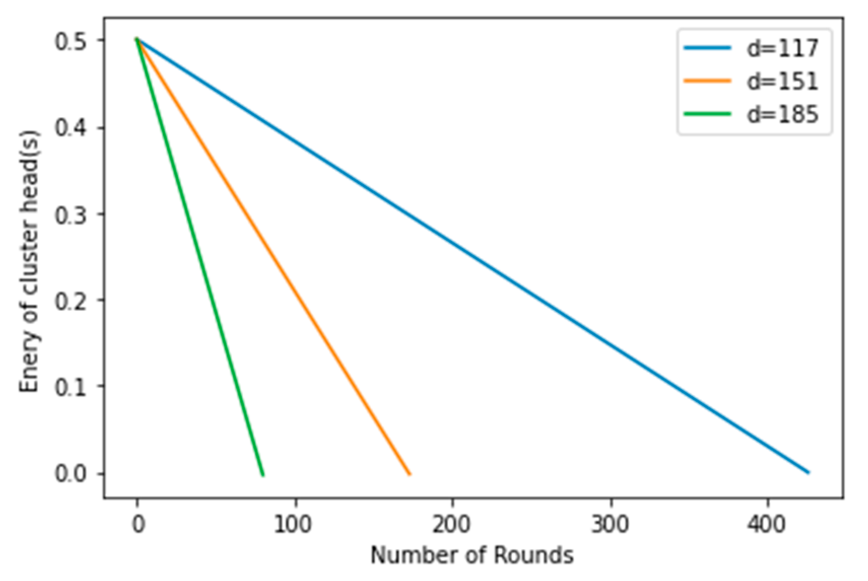
If two CHs are at different distances from the BS, then the transmission energy consumption must be different according to Equation (1). Therefore, in order to equate the transmissions of both the CHs to the BS, we require additional energy for the distant CH. The computation of the additional amount of energy is given in Lemma 2.
Lemma 1.
The cluster head election in FEHCA has a worst-case time complexity of O (Cn2 + Cn CN2 log CN).
Proof: 
The major components in the FEHCA algorithm that dominate the complexity from Step 2 and Steps 3 to 15. As in Step 2, we use the k-means algorithm, which has a complexity of O (CN). Steps 3 to 15 mainly consist of two parts. For Part 1 (Steps 5 to 8), the complexity of this part is O (CN). For Part 2 (Steps 10 to 14), in Step 12, we have used a sorting technique, which has a time complexity of O (CN log CN). Thus, the complete Steps 10 to 14 have a time complexity of O (CN2 log CN). Therefore, the time complexity from Steps 3 to 15 is O (Cn2) + O (Cn CN2 log CN). Now, the overall complexity of Algorithm 1 is O (Cn2) + O (Cn CN2 log CN) + O (CN) ≈ O (Cn2+ Cn CN2 log CN). □
Lemma 2.
Let the energy requirement for the transmission of k-bits from a cluster head (CH) to the base station (BS) in the case of a multipath be  E T x ( k , d ) = k E e l e c + k ε m p d 4 ,   where ‘d’ is the distance between BS and a CH. If the distance between two CHs (CH1 and CH2) from the BS is d1 and d2 such that d2>d1, then, in order to equate the transmissions of CH1 and CH, we need additional energy for CH2, which is given by
Δ =   θ   k ε m p   ( d 2 4 d 1 4 ) k E e l e c + k ε m p d 1 4
where θ is the initial energy with CH1 and CH2.
Proof. 
The energy requirement for transmitting k-bits over the distance d as discussed in Equation (1) is given by:
E T x ( k , d ) = k E e l e c + k ε m p d 4
Since E T x ( ) is a strictly increasing function over ‘d’, E T x ( k , d 2 ) > E T x ( k , d 1 ) for given d2 > d1. Now, using Equation (3), we obtain
k E e l e c + k ε m p d 2 4 > k E e l e c + k ε m p d 1 4
Reversing the inequality in Equation (4) produces
1 k E e l e c + k ε m p d 2 4 < 1 k E e l e c + k ε m p d 1 4
Further, multiplying θ in (5), we obtain
θ k E e l e c + k ε m p d 2 4 < θ k E e l e c + k ε m p d 1 4
Then, equating Equation (6), we obtain
θ + Δ k E e l e c + k ε m p d 2 4 = θ k E e l e c + k ε m p d 1 4
Finally,
Δ =   θ   k ε m p   ( d 2 4 d 1 4 ) k E e l e c + k ε m p d 1 4 .  

5. Results Analysis

In this section of the paper, a simulation setup along with two scenarios is considered. The setup was prepared for the purpose of evaluation of the proposed algorithm (FEHCA). The LEACH and the proposed algorithm were simulated in Python on an Intel Core i5-9300 H CPU @ 2.40 GHz and 8GB RAM running on Windows 10. The sensors were randomly deployed in a 100 m × 100 m area; the initial energy of the sensor was assumed to be 0.5 J. The CH probability was not fixed in advance as in LEACH and was computed at run time, as depicted in Figure 5. FEHCA’s effectiveness was assessed on the same basic parameters as in [37], and the results are shown in Table 1. We tested our proposed algorithm extensively for the following two scenarios and compared the results with the existing LEACH protocol and ESO-LEACH [36].
Scenario 1.
A wireless sensor network (WSN1) is deployed and BS is placed at the middle position (50, 50) in the deployment area (x, y).
Scenario 2.
A wireless sensor network (WSN2) is deployed and BS is placed at position (50, 200), which is far away from the deployment area (x, y).

5.1. Experimental Evaluation for Scenario 1

In Scenario 1, the deployment area (x, y) is 100 m × 100 m, and 100 nodes are deployed at random, with the base station at the centre (50, 50), as shown in Figure 6. Using k-means clustering, the randomly deployed nodes are grouped into an optimal number of clusters, and the centroid of each cluster (marked as ‘x’) is chosen, as shown in Figure 7 and Figure 8.
The results were collected by keeping the base station at position (50, 50) in a 100 m × 100 m area, which was monitored. We first simulated the LEACH algorithm and then the proposed FEHCA with the same simulation parameters and found the proposed algorithm to last, on average, 70 percent longer than the LEACH algorithm, as shown in Figure 9 and Table 2a.
Furthermore, we discovered that, similar to LEACH, most of the nodes in FEHCA were operational for the majority of the time, as shown in Figure 9, whereas this is not the case in many proposed algorithms [36], where the nodes’ batteries start to become depleted immediately, as shown in Table 2b; after a certain number of communication rounds, this forces a decision to be made on the data received from limited regions only. Furthermore, FEHCA lasted 50 percent longer than LEACH, with over 90% of nodes still alive.
The LEACH protocol is valued for its ability to perform with almost all nodes, resulting in higher area coverage for the majority of its lifetime, but its random clustering, unpredictable and random cluster head election mechanism results in high energy dissipation fluctuations, as shown in Figure 10, which must be addressed. Furthermore, LEACH makes no mention of the data packets lost during the algorithm’s operation. FEHCA, on the other hand, addresses both of these issues and the findings are supported by Figure 11 and Figure 12.
The Fault-tolerant Energy-efficient Hierarchical Clustering Algorithm (FEHCA), similarly to LEACH, operates at nearly full strength for the majority of its lifespan, which is critical for reliable networks. It achieves minimum energy dissipation variation due to the determination of optimum number of cluster heads and then by focusing on cluster head placement at or near the centroids, as opposed to LEACH, which elects cluster heads at random. The fault-tolerant behaviour of cluster heads has been also demonstrated by FEHCA. In the event of a cluster head failure, secondary cluster heads (sCHs) take over the task. As shown in Figure 12, failed packet transmissions have been handled and re-transmitted.
In addition, the paper compares FEHCA: H_energy_UD to ESO-LEACH [36] with the same parameters. FEHCA: H_energy_UD uniformly distributes high energy nodes with twice the energy of normal nodes (i.e., 1J initial energy) in each cluster. High energy nodes are contained in the set of N-normal nodes; thus, normal node count = N- high energy nodes.
FEHCA: H_energy_UD, on average, keeps 90% of the network alive for more than 80% of the network life time, while ESO-LEACH keeps around 50% of the network alive for approximately 40% of the network life time, as shown in Table 2b.

5.2. Experimental Evaluation for Scenario 2

In Scenario 2, the deployment area (x, y) is 100 m × 100 m, 100 sensor nodes are randomly deployed and the base station is placed in position (50, 200), i.e., far away from the deployment area, as in hostile environments such as inaccessible border regions, wildlife monitoring, etc., as shown in Figure 13.
Figure 14 shows the clustered network after the optimal clusters have been determined, with the CHs chosen by the BS near or at the centroids. Each cluster communicates directly with the BS with the help of the elected CH, as depicted by Figure 15.
In Figure 16, a typical scenario involving the distance between the BS and the communicating CHs is illustrated, in which three CHs with 0.5 J of initial energy communicating directly with the BS are located at 117 m, 151 m and 185 m distances from the BS. When considering multipath propagation εmp, we can see that the CH furthest from the BS is functional for 80 rounds, while the CHs closer to the BS are able to communicate for 173 and 426 rounds, respectively.
Thus, with knowledge of the distance (di) from the BS and the residual energies (Eres) of the member nodes in the network, a ratio of the energy requirements in accordance with the increasing distance can be formulated to keep the entire monitored area operational. We can compute the lifetime of the closest node in terms of the number of rounds required for it to function, and we can then calculate the energy requirements of the farthest nodes to match the performance in terms of rounds. As a result, as the distance from the base station increases, and we will need to introduce a greater number of high energy nodes.
Due to different energy requirements, cluster heads that are far away from the base station tend to lose energy at a much faster rate than cluster heads that are close to the base station. As a result, after a few rounds of communication with the base station, the network is left with only nearby cluster heads that are communicating with the base station and are responsible for increasing the network lifetime. The simulation results validate this, and is shown in Figure 17.
Based on the distance from the BS and the initial energy known, the lifetime of the nodes closer to the BS and the farthest nodes in terms of number of rounds can be calculated. Furthermore, in accordance with Lemma 2, the ratio of high energy nodes to be deployed as the distance from the BS increases has been determined, and the results are presented in Figure 18, which presents data from distant clusters for the majority of the network lifetime.
Compared to the result of uniform distribution of high energy nodes as shown in Figure 17, the induction of high energy nodes in an increasing manner shows promising results, and the base station is able to receive data from a larger area rather than only from the nearby region, as shown in Figure 18, for a prolonged period of time. This assists in making practical decisions that are much more reliable than decisions made solely on the basis of nearby region cluster heads.
The simulation results depicted in Figure 19, also shows that the proposed FEHCA, with the help of controlled energy dissipation variations due to (a) optimal number of cluster selection, (b) better positioning of cluster heads and (c) energy conservation by delaying the new cluster head election procedure in the case of CH failures, helped in almost doubling the performance as compared to LEACH for the same parameters.
As shown in Figure 19, the proposed algorithm has been tested with high energy nodes that are uniformly distributed (FEHCA: H_energy_UD) and incrementally distributed (FEHCA: H_energy_ID).
When comparing FEHCA and its variants to LEACH, Figure 20 shows the energy consumption variations per transmission, which are again minimised in the case of FEHCA and its variants.

6. Conclusions

Energy conservation and fault tolerance are two major aspects when it comes to wireless sensor networks. This paper presents a centralised clustering mechanism with an energy-efficient data dissemination scheme that can cope with a certain number of faulty cluster heads. We simulated the proposed Fault-tolerant Energy-efficient Hierarchical Clustering Algorithm (FEHCA) for the scenarios with the base station inside as well as outside the monitored area and found the results encouraging. The energy consumption per transmission was much better as compared to LEACH. The proposed FEHCA demonstrated, on average, a 70 percent increase in network performance in terms of the number of rounds as compared to LEACH when the base station was positioned inside the deployment. FEHCA surpassed LEACH in keeping most of the nodes alive for the majority of the time, unlike many well-known proposed schemes with the proper energy management; in fact, FEHCA lasted for 50 percent more rounds than LEACH with more than 90 percent of nodes alive. The proposed algorithm was also compared with ESO-LEACH in terms of common parameters and it succeeded in keeping more than 90 percent of the nodes alive for more than 80 percent of the network lifetime, as compared to ESO-LEACH, where almost 50% of the network was down within approximately 40% of the network lifetime. The algorithm also doubled the communication rounds as compared to LEACH in the case of the base station being placed far away from the deployment. Moreover, with the induction of high energy nodes in an increasing manner in each cluster as per the increasing distance from the base station in accordance with Lemma 2, we observed extended coverage for a prolonged period of time, with the last few sensing nodes left from the entire area to be monitored. FEHCA is also capable of handling lost packets in the case of faulty cluster heads. However, for fault tolerance, FEHCA considers only permanent failures of CHs. In the future, we will attempt to introduce multi-hopping in FEHCA in order to minimise energy consumption and prolong the network lifetime.

Author Contributions

Conceptualization, A.C. and S.K.; Formal analysis, A.C.; Investigation, A.C. and S.G.; Methodology, A.C. and S.K.; Project administration, S.K.; Supervision, S.K.; Validation, A.C. and S.G.; Visualization, A.C.; Writing—original draft, A.C.; Writing—review & editing, S.K., S.G., M.G. and A.M. All authors have read and agreed to the published version of the manuscript.

Funding

This research received no external funding.

Conflicts of Interest

The authors declare no conflict of interest.

References

  1. Akyildiz, I.; Su, W.; Sankarasubramaniam, Y.; Cayirci, E. Wireless sensor networks: A survey. Comput. Netw. 2002, 38, 393–422. [Google Scholar] [CrossRef] [Green Version]
  2. Kumar, S.; Tiwari, U.K. Energy Efficient Target Tracking with Collision Avoidance in WSNs. Wirel. Pers. Commun. 2018, 103, 2515–2528. [Google Scholar] [CrossRef]
  3. Rashid, B.; Rehmani, M.H. Applications of wireless sensor networks for urban areas: A survey. J. Netw. Comput. Appl. 2016, 60, 192–219. [Google Scholar] [CrossRef]
  4. Yick, J.; Mukherjee, B.; Ghosal, D. Wireless sensor network survey. Comput. Netw. 2008, 52, 2292–2330. [Google Scholar] [CrossRef]
  5. Rabaey, J.; Ammer, M.; Da Silva, J.; Patel, D.; Roundy, S. PicoRodio supports ad hoc ultra-low power wireless networking. Computer 2000, 33, 42–48. [Google Scholar] [CrossRef]
  6. Min, R.; Bhardwaj, M.; Cho, S.-H.; Shih, E.; Sinha, A.; Wang, A.; Chandrakasan, A. Low-power wireless sensor networks. In Proceedings of the VLSI Design 2001. Fourteenth International Conference on VLSI Design, Bangalore, India, 7 January 2001. [Google Scholar]
  7. Sohrabi, K.; Gao, J.; Ailawadhi, V.; Pottie, G. Protocols for self-organization of a wireless sensor network. IEEE Wirel. Commun. 2000, 7, 16–27. [Google Scholar] [CrossRef] [Green Version]
  8. Mitchell, T.M. Machine Learning; McGraw Hill: Burr Ridge, IL, USA, 1997. [Google Scholar]
  9. Ayodele, T.O. Types of Machine Learning Algorithms. In New Advances in Machine Learning; Intech: Rijeka, Croatia, 2010; pp. 19–48. [Google Scholar]
  10. Abu Alsheikh, M.; Lin, S.; Niyato, D.; Tan, H.-P. Machine Learning in Wireless Sensor Networks: Algorithms, Strategies, and Applications. IEEE Commun. Surv. Tutor. 2014, 16, 1996–2018. [Google Scholar] [CrossRef] [Green Version]
  11. Kumar, D.P.; Amgoth, T.; Annavarapu, C.S.R. Machine learning algorithms for wireless sensor networks: A survey. Inf. Fusion 2019, 49, 1–25. [Google Scholar] [CrossRef]
  12. Arce, P.; Guerri, J.C.; Pajares, A.; Lázaro, O.; Arce, P. Performance Evaluation of Video Streaming Over Ad Hoc Networks Using Flat and Hierarchical Routing Protocols. Mob. Netw. Appl. 2008, 13, 324–336. [Google Scholar] [CrossRef]
  13. Savvides, A.; Han, C.-C.; Strivastava, M.B. Dynamic fine-grained localization in Ad-Hoc networks of sensors. In Proceedings of the 7th Annual International Conference on Mobile Computing and Networking—MobiCom ’01, Rome, Italy, 21 July 2001; Association for Computing Machinery (ACM): New York, NY, USA, 2001; pp. 166–179. [Google Scholar]
  14. Akkaya, K.; Younis, M. A survey on routing protocols for wireless sensor networks. Ad Hoc Netw. 2005, 3, 325–349. [Google Scholar] [CrossRef] [Green Version]
  15. Heinzelman, W.R.; Chandrakasan, A.; Balakrishnan, H. Energy efficient communication protocol for wireless microsensor networks. In Proceedings of the 33rd Annual Hawaii International Conference on System Sciences, Maui, HI, USA, 7 January 2000; pp. 1–10. [Google Scholar]
  16. Yassein, M.B.; Khamayseh, Y.; Mardini, W. Improvement on LEACH protocol of wireless sensor network (VLEACH). Int. J. Digit. Content Technol. Appl. 2009, 132–136. [Google Scholar] [CrossRef] [Green Version]
  17. Mahapatra, R.P.; Yadav, R.K. Descendant of LEACH Based Routing Protocols in Wireless Sensor Networks. Procedia Comput. Sci. 2015, 57, 1005–1014. [Google Scholar] [CrossRef] [Green Version]
  18. Fanian, F.; Rafsanjani, M.K. Cluster-based routing protocols in wireless sensor networks: A survey based on methodology. J. Netw. Comput. Appl. 2019, 142, 111–142. [Google Scholar] [CrossRef]
  19. Chan, L.; Chavez, K.G.; Rudolph, H.; Hourani, A. Hierarchical routing protocols for wireless sensor network: A compressive survey. Wirel. Netw. 2020, 26, 3291–3314. [Google Scholar] [CrossRef]
  20. Li, X.; Wang, J.; Bai, L. LEACH Protocol and Its Improved Algorithm in Wireless Sensor Network. In Proceedings of the 2016 International Conference on Cyber-Enabled Distributed Computing and Knowledge Discovery (CyberC), Chengdu, China, 13–15 October 2016; pp. 418–422. [Google Scholar]
  21. Razaque, A.; Abdulgader, M.; Joshi, C.; Amsaad, F.; Chauhan, M. P-LEACH: Energy efficient routing protocol for Wireless Sensor Networks. In Proceedings of the 2016 IEEE Long Island Systems, Applications and Technology Conference (LISAT), Farmingdale, NY, USA, 29 April 2016; pp. 1–5. [Google Scholar]
  22. Alnawafa, E.; Marghescu, I. IMHT: Improved MHT-LEACH protocol for wireless sensor networks. In Proceedings of the 2017 8th International Conference on Information and Communication Systems (ICICS), Irbid, Jordan, 4–6 April 2017; pp. 246–251. [Google Scholar]
  23. Khan, M.K.U.; Ramesh, K.S. A Modified LEACH Algorithm for WSN: MODLEACH; Springer Science and Business Media LLC: Berlin/Heidelberg, Germany, 2019; pp. 632–642. [Google Scholar]
  24. Tong, M.; Tang, M. LEACH-B: An Improved LEACH Protocol for Wireless Sensor Network. In Proceedings of the 2010 6th International Conference on Wireless Communications Networking and Mobile Computing (WiCOM), Chengdu, China, 23–25 September 2010; pp. 1–4. [Google Scholar]
  25. Chen, J. Improvement of LEACH Routing Algorithm Based on Use of Balanced Energy in Wireless Sensor Networks. In Computer Vision; Springer Science and Business Media LLC: Berlin/Heidelberg, Germany, 2011; Volume 6838, pp. 71–76. [Google Scholar]
  26. Xu, J.; Jin, N.; Lou, X.; Peng, T.; Zhou, Q.; Chen, Y. Improvement of LEACH protocol for WSN. In Proceedings of the 2012 9th International Conference on Fuzzy Systems and Knowledge Discovery, Chongqing, China, 29–31 May 2012; pp. 2174–2177. [Google Scholar]
  27. Tripathi, M.; Gaur, M.; Laxmi, V.; Battula, R.B. Energy Efficient LEACH-C Protocol for Wireless Sensor Network. In Proceedings of the Third international conference on Computational Intelligence and Information Technology (CIIT 2013) Institution of Engineering and Technology (IET), Mumbai, India, 18–19 October 2013; pp. 402–405. [Google Scholar]
  28. Anandamurugan, S.; Abirami, T. Antipredator Adaptation Shuffled Frog Leap Algorithm to Improve Network Life Time in Wireless Sensor Network. Wirel. Pers. Commun. 2016, 94, 2031–2042. [Google Scholar] [CrossRef]
  29. Singh, S.P.; Sharma, S. An improved cluster-based routing algorithm for energy optimisation in wireless sensor networks. Int. J. Wirel. Mob. Comput. 2018, 14, 82. [Google Scholar] [CrossRef]
  30. Mechta, D.; Harous, S.; Alem, I.; Khebbab, D. LEACH-CKM: Low Energy Adaptive Clustering Hierarchy protocol with K-means and MTE. In Proceedings of the 2014 10th International Conference on Innovations in Information Technology (IIT), Al Ain, United Arab Emirates, 9–11 November 2014; pp. 99–103. [Google Scholar] [CrossRef]
  31. Azharuddin, M.; Kuila, P.; Jana, P.K. Energy efficient fault tolerant clustering and routing algorithms for wireless sensor networks. Comput. Electr. Eng. 2015, 41, 177–190. [Google Scholar] [CrossRef]
  32. Bhatti, D.M.S.; Saeed, N.; Nam, H. Fuzzy C-Means Clustering and Energy Efficient Cluster Head Selection for Cooperative Sensor Network. Sensors 2016, 16, 1459. [Google Scholar] [CrossRef] [PubMed]
  33. Azharuddin, M.; Jana, P.K. PSO-based approach for energy-efficient and energy-balanced routing and clustering in wireless sensor networks. Soft Comput. 2016, 21, 6825–6839. [Google Scholar] [CrossRef]
  34. Parwekar, P.; Rodda, S.; Mounika, S.V. Comparison between Genetic Algorithm and PSO for Wireless Sensor Networks. In Smart Computing and Informatics; Springer: Singapore, 2018; pp. 403–411. [Google Scholar] [CrossRef]
  35. Saveros, F.; Gong, M.; Carlsson, N.; Mahanti, A. An energy-efficient handover algorithm for wireless sensor networks. In Proceedings of the 2016 IEEE 35th International Performance Computing and Communications Conference (IPCCC), Las Vegas, NV, USA, 9–11 December 2016; pp. 1–8. [Google Scholar]
  36. Nigam, G.K.; Dabas, C. ESO-LEACH: PSO based energy efficient clustering in LEACH. J. King Saud Univ. Comput. Inf. Sci. 2018. [Google Scholar] [CrossRef]
  37. Heinzelman, W.; Chandrakasan, A.; Balakrishnan, H. An application-specific protocol architecture for wireless microsensor networks. IEEE Trans. Wirel. Commun. 2002, 1, 660–670. [Google Scholar] [CrossRef] [Green Version]
  38. Muhammed, T.; Shaikh, R.A. An analysis of fault detection strategies in wireless sensor networks. J. Netw. Comput. Appl. 2017, 78, 267–287. [Google Scholar] [CrossRef]
  39. Sasikumar, P.; Khara, S. K-Means clustering in wireless sensor networks. In Proceeding of the 2012 Fourth International Conference on Computational Intelligence and Communication Networks, Mathura, India, 3–5 November 2012; pp. 140–144. [Google Scholar]
Figure 1. Typical hierarchical architecture.
Energies 14 03935 g001
Figure 2. Depiction of random distribution of cluster heads in conventional LEACH protocol.
Energies 14 03935 g002
Figure 3. Scenario where most of the area is unmonitored in a live network.
Energies 14 03935 g003
Figure 4. Timeline showing the overall operation of the algorithm.
Energies 14 03935 g004
Figure 5. Optimal number of clusters in the network.
Energies 14 03935 g005
Figure 6. Random deployment of 100 sensor nodes in an area of 100 m × 100 m with BS positioned inside the deployment area.
Energies 14 03935 g006
Figure 7. Network clustering using k-means algorithm.
Energies 14 03935 g007
Figure 8. Depiction of network clusters with centroids.
Energies 14 03935 g008
Figure 9. Performance of FEHCA and LEACH in terms of operational nodes per round when base station is positioned inside the deployment area.
Energies 14 03935 g009
Figure 10. Energy dissipation per round in LEACH.
Energies 14 03935 g010
Figure 11. Energy dissipation comparison per round in LEACH and FEHCA.
Energies 14 03935 g011
Figure 12. Retransmissions per round in FEHCA.
Energies 14 03935 g012
Figure 13. Random deployment of 100 sensor nodes in an area of 100 m × 100 m with BS positioned outside the deployment area at position (50, 200).
Energies 14 03935 g013
Figure 14. Network clustering using k-means algorithm.
Energies 14 03935 g014
Figure 15. Depiction of network clusters along with respective centroids (each cluster communicates directly with the BS).
Energies 14 03935 g015
Figure 16. Effect of distance of cluster heads (CHs) from BS on the network lifespan.
Energies 14 03935 g016
Figure 17. Placement of alive nodes when the count is less than 10 with uniform distribution of high energy nodes.
Energies 14 03935 g017
Figure 18. Placement of alive nodes when the count is less than 10 with incremental distribution of high energy nodes.
Energies 14 03935 g018
Figure 19. Performance of FEHCA and LEACH in terms of operational nodes per round when BS is positioned outside the deployment area.
Energies 14 03935 g019
Figure 20. Energy dissipation per round in LEACH and FEHCA when BS is positioned outside the deployment area.
Energies 14 03935 g020
Table 1. Simulation parameters for FEHCA.
ParametersValues
Area100 m × 100 m
Number of nodes100
Sink locationcentre and 50,200
Optimal cluster ratio (Cr)07
Initial energy of node, Ei0.5 J
Data packet size4000 bits
Energy consumption: power amplifier, εfs10 × 10−12 J/bit/m2
Energy consumption: power amplifier, εmp0.0013 × 10−12 J/bit/m4
Energy dissipated to run the transmitter or receiver circuitry, Eelec50 × 10−9 J/bit
Energy consumption: aggregation (EDA)5 × 10⁻⁹ j/bit/signal
Threshold distance, do87.7 m
Initial energy of high energy node1 J
Table 2. (a) Network lifetime comparison of LEACH and FEHCA; (b) network lifetime comparison of ESO-LEACH and FEHCA:H_energy_UD.
(a)(b)
No. of RoundsNo. of Alive Nodes in LEACHNo. of Alive Nodes in FEHCANo. of RoundsNo. of Alive Nodes in ESO- LEACH [36]No. of Alive Nodes in FEHCA:H_energy_UD
10010010010010099
200100992009399
300100993008899
400100994008599
500100995008199
600100976007199
700100967006499
75089968005799
80039959005198
85009410004598
900 9311003798
1000 9312003298
1100 92130028 *93
1150 73135024 *13
1200 051500185
1300 05165013 *0
1350 04180010
1400 0220004
1450 022000
* Approximate values ascertained from the results [36].
Publisher’s Note: MDPI stays neutral with regard to jurisdictional claims in published maps and institutional affiliations.

