Sound Localization for Ad-Hoc Microphone Arrays

Abstract

Sound localization is a field of signal processing that deals with identifying the origin of a detected sound signal. This involves determining the direction and distance of the source of the sound. Some useful applications of this phenomenon exists in speech enhancement, communication, radars and in the medical field as well. The experimental arrangement requires the use of microphone arrays which record the sound signal. Some methods involve using ad-hoc arrays of microphones because of their demonstrated advantages over other arrays. In this research project, the existing sound localization methods have been explored to analyze the advantages and disadvantages of each method. A novel sound localization routine has been formulated which uses both the direction of arrival (DOA) of the sound signal along with the location estimation in three-dimensional space to precisely locate a sound source. The experimental arrangement consists of four microphones and a single sound source. Previously, sound source has been localized using six or more microphones. The precision of sound localization has been demonstrated to increase with the use of more microphones. In this research, however, we minimized the use of microphones to reduce the complexity of the algorithm and the computation time as well. The method results in novelty in the field of sound source localization by using less resources and providing results that are at par with the more complex methods requiring more microphones and additional tools to locate the sound source. The average accuracy of the system is found to be 96.77% with an error factor of 3.8%.

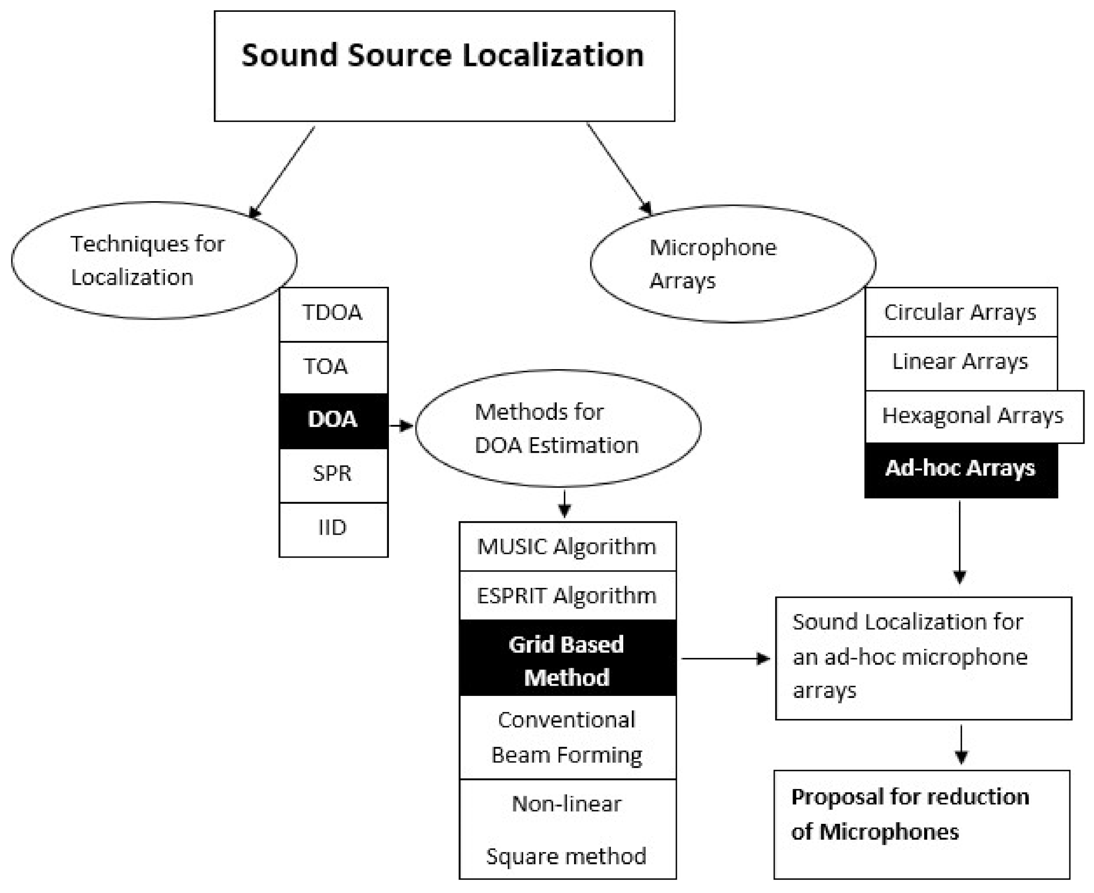
1. Introduction

Sound source localization deals with determination of the location from where a sound signal is originated with respect to an array of microphones [1]. Sound localization is an important and useful research field which has been used in many different applications in the past decades [2]. This method has been measured by using time difference of arrival since the World War 1 [3]. Even today, many of the speech and voice recognition systems utilize the knowledge of sound source location [2]. With the wide use of cameras and microphones in every other application, a lot of research is conducted within this industry [4].

Many different signal processing algorithms that have been proved to be efficient and that consumes less energy are used extensively. One of these algorithms is sound localization, which is an example of collaborative signal processing [5]. Widely used source localization methods work by determining the direction of sound waves coming from the source and finding the distances between sensors and source [6]. Incoming sound waves provide the horizontal and vertical angles for the direction, which assists in source location. For sound localization, sounds are divided into three coordinate systems. The first is the azimuthal or horizontal coordinate system, which include the sounds that are either to the right or left side of the sensor and are detected by the time or level difference of sounds on each sensor node. The second coordinate system is the elevation or vertical coordinate system, which tells whether the incoming sound is present above or below the sensor and these waves are detected by the use of the difference in the frequency of sound as the waves bounce causing the difference in frequency. The third system is the use of distance measurement which still requires much research because different distance cues are used. In the case of ears, which are sound sensors for humans, four different distance cues are used which include reflection, sound frequency, movement parallax and sound level [7].

Microphones are arranged in an array to further increase the sound quality. Sound localization microphone arrays utilize multiple microphones that are used to perform different types of signal processing by utilizing the concept of phase difference of sound waves [8]. These arrays assume that the placement of microphones is regular and the channels are synchronized with multichannel analog to digital converter. All microphones in the array are time synchronized and are arranged in a particular geometry for the correct determination of location. This process of sound source localization is based on time delay [4]. Sound source localization has many advantages in robotics which assists the robots in detecting sound source by using only sound; this helped in enhancing the human-robot interactions.

The advancements made in this field gave rise to various type of microphone arrays which assisted in improving quality and precision. One such type of microphone arrays is the ad-hoc microphone array. Such arrays include one or more microphones which cannot communicate with each other [9]. This type of microphone arrays can be best explained by the example of different laptops in a meeting [10]. Every laptop has set of built in microphones of its own along with the Wireless Fidelity (Wi-Fi) enabling feature. This set of arrangement in an ad-hoc fashion can form a network [4]. Ad-hoc microphone arrays are closer to other participants and are spatially distributed which further improves sound quality. Placement of ad-hoc microphones is also closer to the speakers which helps in obtaining more accurate source localization. Bearing the advantages of ad-hoc microphones in mind, there also exists certain issues in this fashion out of which synchronization is a major problem. All the microphones that belong to different persons are not synched. Different microphones may have different gains that are sometimes unknown. Connected microphones also have different signal to noise ratios [4].

The synchronization issue is solved through many different techniques. One of which is by the use of dedicated links. All the individual microphones send the special synchronized signal over to this dedicated link. To overcome the issues of geometry of microphones, a coded chirp is produced by each loudspeaker [11].

Microphone arrays are used extensively in many devices such as teleconferencing and hearing aids. There still exists some constraints of power, space and processing which hinders the performance of these arrays [12]. Currently, much attention is given to the ad-hoc microphones because they use multiple recording devices for multichannel processing. Ad-hoc arrays are considered better than simple microphone arrays because they do not require large scale recording devices and provide freedom in the choice of recording devices [13]. However, in this project we demonstrate the use of a predetermined arrangement of microphones with the source to resolve the problem of how the experimental arrangement should be conducted to localize source in case of four microphones.

In this study, the method DOA is used to estimate the position and constraints of the source location. This method has been used by a numerous number of nodes and it is required to be modified on two separate nodes such that there are two microphones arranged in each node. This technique provides the same location accuracy and precision [14].

This system forms its basis from the fact that, in reality, we have two ears which act as the sensor nodes and provide us with the knowledge of sound source location. Utilizing the same concept, implementing it on microphones is a crucial task and is of great importance as the stability of the desired system will result in many useful products, such as hearing aids for the disabled.

Localization of sound mainly involves two steps which are:

(i)

Direction of arrival estimates;

(ii)

Distance estimates.

Both of these estimates are carried out separately and different mapping procedures are used for the correct knowledge of this information [15]. For a better and concise understanding of this document, Figure 1 illustrates the steps taken in order to develop a framework for the project and presents an overview of the whole study.

The basic aim of this project is to localize a single sound source and retrieve data from it by using a novel arrangement of microphone arrays. Sound localization using four microphones is performed using different methods. Localizing a sound source by using a lesser number of nodes (two or three) is the prime objective of the project. Stability of the system using two or three nodes is crucial. The proposed system addresses the existing problems identified in the research and thus makes the following contributions:

• To test a configuration of sensors with a source that requires a minimum number of microphones, to reduce the complexity of the system and to decrease the resource consumption. Previously, this task has been accomplished using six microphones [16]. This study further reduces the number of microphones to four in order to minimize the resource consumption.
• To localize a source accurately by using both DOA and 3D localization. The study proposes novel methods to calculate these.
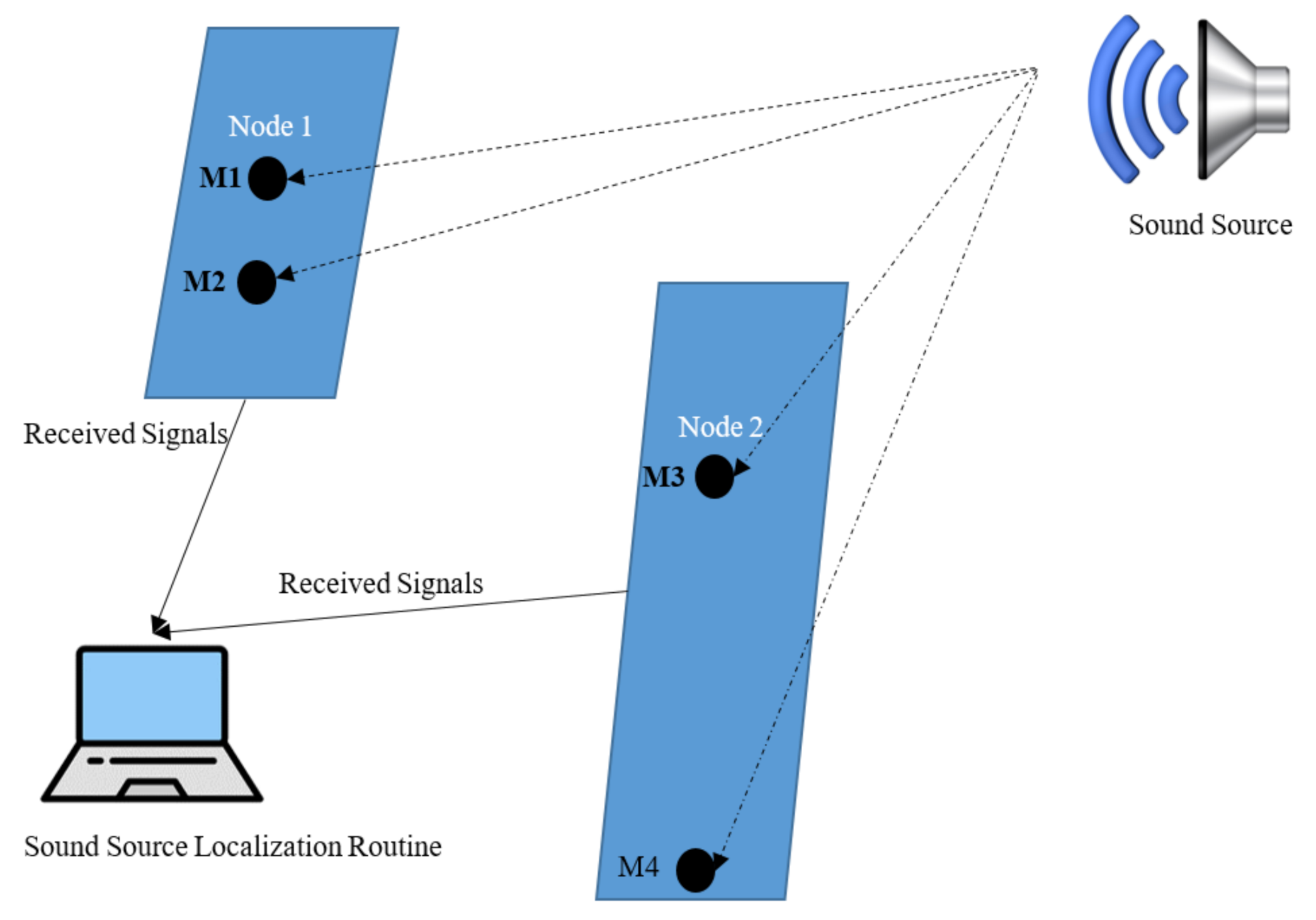
• To develop a sound localization system possessing only two nodes so that it could be compact and be ready to be integrated in devices such as hearing aids.
• The system is particularly developed to work in reverberant environments where there is excessive noise content. The purpose is achieved by adding noise to the input signals and calculating the error factor.

This paper is organized as follows: The following section explains the process of sound localization by the method of DOA along with the advancement for implementation of this system on a lesser number of nodes. It also discusses the approach of using lesser nodes for the localization and proposal for the implementation of a stable two node system which works as efficiently as a four node system. Section 3 presents the results of the implemented source localization routine. Section 4 presents the conclusion of the study and summarizes the results and achievements. Section 5 discusses the overall study, contribution and results. Section 6 presents future work indicating possible future directions and potential improvements.

2. Related Work

According to the recent literature, sound source can be located by finding time delays between the signals arriving at the microphones [17,18,19]. In a method called bi-channel sound source localization, only a single pair of microphones is used as discussed in [20,21,22,23]. This method calculates the inter-aural time difference between signals to find the azimuth angle. The techniques proposed in such studies are based on the assumption that the source of sound is located parallel to the microphone on the horizontal axis. However, these approaches are inherently restricted to localizing sound in only one dimension. Some techniques have been developed to determine both azimuth and height [24,25], while tracking of source signals have been performed in [26,27]. In these approaches, an impulse response function has been estimated. This function integrates both room-impulse-response (RIR) and a head-related-transfer-function (HRTF) [28]. To ensure that the system is adaptable, the inherent characteristics of the microphone used in the HRTF should be calculated independently from the auditory characteristics of the environment that has been exhibited by RIR. Another limitation is that these methods are computationally extensive, as the sound localizing approaches used in them do not deliver closed-form expressions. Furthermore, the location of the source have a highly complicated reliance on HRTF and RIR. Hence, it is hard to determine the measure of this dependency. It can be concluded that there are two major limitations of these methods. First, they require huge datasets for training and intricate processes for learning. Second, the determined factors are relevant to a specific mixture of location of the microphones, their angles and the characteristics of the environment where they are used. For all viable combinations, the determination of these factors is not realistic. This render these methods difficult to be adapted and incorporated in new environments.

Another group of techniques known as multilateration performs sound source localization using Time Delay Estimation (TDE) by leveraging two or more microphones. In these methods, TDE factors are calculated pair-wise and the source is finally localized using these factors. TDE does not depend on the position of microphones or source. This implies that the two stages of calculating TDE and localizing sound source are independent of one another. In addition to that, the geometry of the array of microphones is not incorporated by the TDEs. This means that the TDE factors are calculated independent of the location of the microphones. However, this property is challenging as it is not certain that a source coordinate exists that is stable with all TDEs. This probable limitation can be demonstrated by an example where a set of three microphones are used which form a linear array. In this experiment, $t_i$ is the time of arrival (TOA) at the $i$th microphone and $t_{i:j}=t_j-t_i$ represents the time delay related to the pair of microphones (i,j). In the specific case of a linear array comprised if three microphones, the conditions $t_{1,2}>0$ and $t_{3,2}>0$ do not hold true. Hence, it can be inferred that the sound signals arrive at the first and third microphones before arriving at the middle microphone. This is not consistent with the path of transmission of the sound signal. To solve this problem, the Maximum Likelihood (ML) method has been designed to achieve multialteration in [29,30,31,32,33,34,35]. In these studies [36,37,38,39,40,41], this method is proposed in the form of least squares. In [42,43,44,45], this concept has been implemented as global coherence fields (GCF). Various TDE and sound source localization methods have been evaluated using the multiateration approach. This has paved the path for understanding the relationship among sound source localization and TDE in a better manner. If the outliers of TDE have been eliminated by the above mentioned methods, the occurrence of these outliers cannot be entirely prevented or reduced. Furthermore, in the environments having high noise content the performances of these methods are greatly reduced [46].

Multichannel sound source localization is another class of methods that determines all of the time delays simultaneously, which means that the common stability of the system is ensured. This category is divided into two subcategories. In the first subcategory, the impulse responses of sound waves are used to calculate TDEs in order to localize the sound source [47,48,49,50,51]. The limitation of these techniques is that it is very difficult to estimate the impulse responses using unprocessed data since raw data has been used to calculate the responses.

Sound source localization problems in a shallow water environment have been tackled in [52]. In this study, a convolutional neural network (CNN) has been used to localize sound sources of noise radiating on the sea floor. According to results, CNN, while working with cepstrogram, is capable of accurately localizing sound signals and estimating their range. An et al. proposed a reflection based technique to perform sound source localization in three-dimensional environment [53]. Both direct and indirect sound waves arriving at the microphones are considered in the experiments. The indirect signals are those, which are reflected by matters such as ceilings or walls. Monte Carlo localization technique has been used to perform sound source localization. The paths of sound signals have been determined using the sound beams tracing approach. A 40% increase in the accuracy of the sound localization method has been recorded by using indirect sound waves along with the direct ones. An approach using thin resolution networks have been proposed in [54]. The authors developed a microphone model based on directivity to determine the invalid microphones and to minimize the number of directions. A 3D Kalman method was modified to perform 3D localization of sound sources. Learning based sound source localization has been explored by Opochinsky [55]. First, sound attributes are first taken as input from the captured signals. These features are inputted to a system that locates them with respect to the location of the sources. A deep learning model is used, which uses a small amount of data samples that are labelled according to their positions, and another set of unlabeled data is utilized in which only the relative location is known [56]. The deep learning model associates sound features to the source’s angle of azimuth. Evers et al. worked on dynamic sound source localization. In such an environment, the sound source and microphone pairs may be in a state of motion. The changes in the source and sensor orientation also further affect these signals. To minimize errors and false detection in such scenarios, a Localization and Tracking (LOCATA) framework has been developed [57].

In order to calculate the sound field at various locations of microphones and assess the properties of the noise sources, acoustic imaging algorithms have been widely used [58]. Relative to the techniques belonging to this domain, the data is collected using the sound propagation model by the array of microphones [59]. This data is then used to assess the properties of the sound source. The beamforming technique is one of the fundamental methods for the sound data captured by the microphones [58,60]. However, this method, in normal circumstances, does not give good results for real-world programs. The geometry of the microphone array limits the quantification of the sources of sound. The majority of acoustic imaging techniques can be termed as exhaustive search methods. In these approaches, a specific grid is scanned to identify the location of the sound source. One limitation of such methods is the high cost of computation since they are relatively more sophisticated [61,62,63,64,65,66,67,68,69,70,71,72,73,74]. Recently Munawar et al. has worked on acoustic imaging in [75,76,77,78,79]. His method involves generating imageries of the inner structure of an object using ultrasound [80,81,82,83,84].

In the recent literature, the approaches for sound quantification is related with measurement of sound properties such as intensity, frequency, sensitivity, spectrum and pitch [85]. In [86], noise quantification of aircraft parts has been conducted using moving microphone arrays. The microphones are arranged in the form of concentric rings. A modified beamforming method using delay and sum strategy has been used, which includes finding the microphone correlations. In [87], a fly over microphone array has been used for the sound measurement of a flying aircraft. Beamforming methods based on phased arrays have been proposed to locate sound sources. The problem of sound estimation from distributed sources has been addressed in [88]. An extension of the Source Power Integration (SPI) method called SPIL has been used along with sensitivity analysis to locate line source emitting trailing edge noises.

3. Materials and Methods

3.1. Materials

The experiments were conducted in a laboratory environment. The experimental arrangement consisted of four microphones and a sound source. An HP Envy x360 laptop with Intel Core i7-7200U CPU, clock speed of 2.70 GHz and 8 Gigabytes RAM was used. A LABView 2020 application was run on the Windows 10 operating system. This program captures sound signals from the microphones and saves them in an Excel spreadsheet. The saved sound signals are then used by the sound source localization routine developed in MATLAB programming language in the MATLAB R2013b framework.

3.2. Assumptions

Before performing the sound source localization experiment, we made the following assumptions:

• Only one omni-directional and little sound source is present.
• Reflection of sound waves take place between the plane where the source and the neighboring items are located.
• There are no noise elements in the environment. The sound signal contains the level of noise deemed acceptable for the experiment.
• All microphones have matching phase and amplitudes.
• There are no self-producing noises in any of the microphones.
• The locations of audio sensing devices are predetermined.
• The difference in the velocity of sound caused by fluctuations in physical characteristics such as pressure and temperature are ignored.
• Sound velocity in the air is considered to be 330 m per second.
• The sound signals arriving at the sensors will be considered as planar rather than spherical in the case where the distance between the source and the sensors surpasses the gap between the microphones.

3.3. Background

The basic idea of sound localization works in a simple method of receiving the sound from the source and then extracting the useful information which assists in the detection of the target. These features differ depending on the model, which is used in particular applications. Performing different estimations, accordingly, provide the localization results. Basic steps, which are taken in the whole process, are given in Figure 2.

Considering the advantages of DOA in reference, it is the best suited method for the sound localization task since it is bandwidth efficient and can work with unsynchronized input unless the motion is relatively slow. There are many methods present in the literature for implementing DOA, which includes Independent Component Analysis, ESPRIT algorithm and MUSIC algorithm to name a few. For our application we chose to implement DOA estimation using the grid-based method [62].

3.3.1. Direction of Arrival Estimation

The classical techniques for finding the DOA fall into two categories, which are (1) beamforming and (2) high resolution-based procedure. The high-resolution method has limitations in terms of complex computations and lacks consistent results [63]. Due to such shortcomings, the beam forming is given preference for DOA estimation in many applications. In time and frequency fields, the beam-forming based method provides a more accurate calculation of DOA. Another noteworthy method using beamforming is the distribution method of spatial time-frequency, which has been used in the literature [64]. In the frequency field, the DOA calculation utilizing beamforming requires double estimation of Fast Fourier Transform (FFT). First, FFT is applied to achieve the frequency spectrum of the input sound wave. During the second time, FFT is applied to obtain the estimated value of DOA. The length of data determines the frequency resolution of FFT. Due to this, the estimation of DOA depends on the array size or the amount of elements in the array. If the data lengths are small, the accuracy of the computed DOA value will decline. This paper targets this problem of DOA estimation using beamforming that exists in the literature. In the frequency field, a method to calculate the phase difference is presented for the determination of the DOA of a signal. Using such a technique, the limitation involving the array size in the method based on space-frequency is reduced. In our experiments, this method showed a more precise resolution of DOA.

3.3.2. Model of a Signal

Consider an arrangement where a total of n microphone arrays record m narrow band sound signals where (n > m). Here the elements of these arrays are microphones, which are placed at a distance of r from one another. The wavelength of the signal is denoted by ${\mathsf{\lambda }}_j$, where j = 1, 2, 3, …, m. Its DOA will be ${\theta }_j$ (j = 1, 2, 3, …, m). Using this information, the phase difference is mathematically represented using the following equation:

$${\omega }_j=2\pi \frac{r}{{\mathsf{\lambda }}_j} \sin {\theta }_j$$

(1)

and high-resolution and the direction vector will be given as follows.

$$d{\left(\omega \right)}_j={\left[1 e^{-i{\omega }_j} e^{-i2{\omega }_j}\dots e^{-i\left(n-1\right){\omega }_j}\right]}^T$$

(2)

The received signal will be given as follows.

$$a\left(t\right)=X\left({\omega }_j\right) s\left(t\right)+p\left(t\right)$$

(3)

From the above equation, $X\left({\omega }_j\right)$ represents the following.

$$X\left({\omega }_j\right) =[ a\left({\omega }_1\right),a\left({\omega }_2\right), \dots , a\left({\omega }_m\right)]$$

(4)

The value s(t) represents the source signal, which is represented by the following.

$$s\left(t\right) ={[s_1\left(t\right), s_2\left(t\right),\dots , s_m\left(t\right)]}^T$$

(5)

The value p(t) denotes white noise which will be represented as follows.

$$p\left(t\right) =[p_1\left(t\right), p_2\left(t\right),\dots , p_m\left(t\right)]$$

(6)

3.3.3. Spatial Frequency Distribution for the Estimation of DOA

The function of a spatial filter can be achieved by a beam shaper. The spatial frequency of the source signal can be represented by the direction of the source signal in 3D space. The frequency response of the filter can be considered as the direction of the wave beam. The center frequency of the spatial filter will be represented by the highest value of the wave beam.

In order to form the spatial signal, we use M wave beams. The spatial frequency of the signal will correspond to the mth wave beam if the mth wave beam’s output is the highest. This indicates that the FFT of the output of the array elements taken simultaneously will create a spatial filter, that is, spatial multi-beam. In the frequency domain, the execution of the beam forming process requires a double application of FFT. For the first time, a FFT is applied to the output of the array elements in the time domain. This will give the frequency range of the signal element. On the second application of FFT, the spatial FFT of the Fourier coefficients of the array elements is then calculated to an equal frequency, which enables the output to form a spatial multi-beam. We consider the example of two signals as represented below.

$$x_1\left(t\right)=\cos \left(2\pi f_{1}t\right)$$

(7)

$$x_2\left(t\right)=\cos \left(2\pi f_{2}t\right)$$

(8)

The values of $f_1$ and $f_2$ are taken as 150 Hz and 200 Hz, respectively. The DOAs of the signals are measured as 30 degrees and 60 degrees, respectively. There is a total of 10 array elements, indicating that n = 10, for receiving the signals placed with a distance of 0.45 m between them. The noise element $p_i\left(t\right)$ of each element of the array is white noise. The signal to noise ratio (SNR) is 7 db. We applied FFT to the output of the first element of the array. The resulting waveform is shown in Figure 3.

From Figure 3, the frequencies of the two signals can be obtained, which will be used to calculate their wavelengths. Each array element’s peak value will be used to construct a new series given as: $F_1$, $F_2$, $F_3$, …, $F_n$. Then, FFT will be applied to the new series. The resultant frequency distribution is shown in Figure 4.

From the above figure it is evident that DOA has a large error factor. In this figure, the value of $\sin {\theta }_2$ is greater than one, which is certainly false. By increasing the number of array elements, a more precise value of DOA is obtained. Hence, we can see that the precision of the calculated DOA value is directly proportional to the number of array elements. However, in real life applications the number is usually limited and it is not practical to increase the array elements to a large value. This implies that in order to calculate the DOA value in the frequency domain, a more precise and less complex method is required. In order to solve this problem, we proposed the concept of using phase differences to calculate DOA in the frequency domain.

3.3.4. DOA Calculation Using Phase Differences

As the conventional phase difference method used for DOA estimation depends too much on the array size and requires a large number of elements in the arrays for accuracy, we used an alternative method for DOA calculation. This method is simpler, requires fewer resources and takes less computational time than the traditional approach. The experimental set up involves three nodes or arrays of microphones, where there are three microphones in each array. The sound waves recorded by these microphones are saved and the phases among each sequence of signals are determined. This implies that the phase between the signals recorded by each element of the array are computed. The MATLAB formula for computation of phases is given as:

phase = acos(dot(v1,v2)/(norm(v1)*norm(v2)))

(9)

where v1 and v2 are vectors representing the two recorded signals. The dot product of these vectors is divided by the products of their normalized forms and results in the estimated phase value. The phases are further used to calculate phase differences. The phase differences are used to calculate the angle of arrival or DOA using the following equation.

$$\theta =\frac{\mathrm{asin}\left(p\lambda \right)}{2\pi }$$

(10)

In this equation, p represents the phase difference between the sound waves. As there are multiple values of the calculated phase differences, there were two values of the angle θ. The final value of DOA was calculated by taking an average of these two angles.

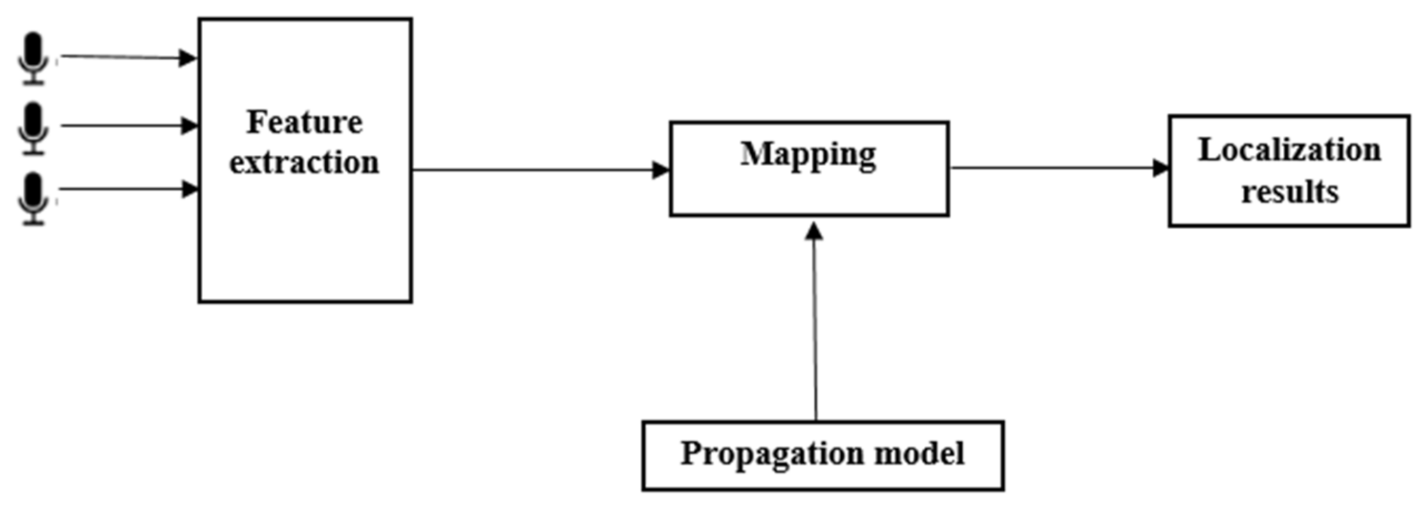
3.3.5. Source Localization in 3D Space

Previously sound localization has been implemented in 3D space using an XYZO microphone array [74]. The microphone array used in this research was based on both bidirectional and omni-direction microphones. This arrangement was referred to as the world’s smallest array of microphones in the air for the localization of sound in 3D space. The configuration of this microphone array has been performed and the array is calibrated for the 3D modeling of source. Hence, this microphone array possesses a significantly reduced size compared with other systems. The implementation involved computing the widely used DOA and searching the source in 3D space as well. A GPU platform has been used to speed up the computations in parallel. A multi-threaded CPU implementation was performed with 130X speed up. The system was programmed in CUDA programming. This system was experimented by using different levels of mixtures in noise and signals. This research incorporates another microphone array to this configuration in order to improve results as well as to render the system compatible for use in hearing aids and to render sound source localization possible to be used with the two human ears.

The sound localization routine proposed in this research is based on two microphone arrays, with two microphones in each array. The total number of microphones in the configuration is four. The microphones are arranged in the shape of a tetrahedron. A sound source is formed by mixing sound signals from two different sources. These sources are speech sound waves from two different speakers. The resultant sound wave is then mixed with some noise. This procedure is performed to mimic the practical environment where multiple people are speaking with moderate noise levels present at the background. The coordinates of microphones in 3D space are hardcoded in the program. The MATLAB implementation of code then uses the time delay of the arrival of the source sound signals at the microphones to determine the source location. The working of this system under varying circumstances is performed to test its robustness.

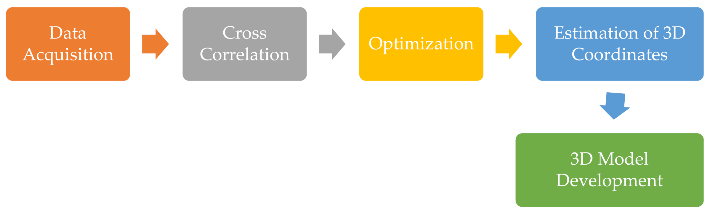
3.4. Proposed Method

The proposed research extends this microphone configuration for 3D sound localization by adding another node to the apparatus. This node consists of an array of two microphones. This renders the total number of microphones in the system to four. There are two nodes of microphones. In each node there is an array of two microphones. Such a configuration adds to the precision of the sound localization routine. It also renders it compatible to be used in hearing assistance devices such as hearing aids, which are worn on two ears. The source sound wave is formed by mixing sound from two sources. Each source contains a recorded speech of a person. The resultant sound signal has been mixed with noise to mimic the sound signals produced in real time scenarios where multiple people are speaking with some levels of noise in the background. The process followed for source localization has been summarized in Figure 5.

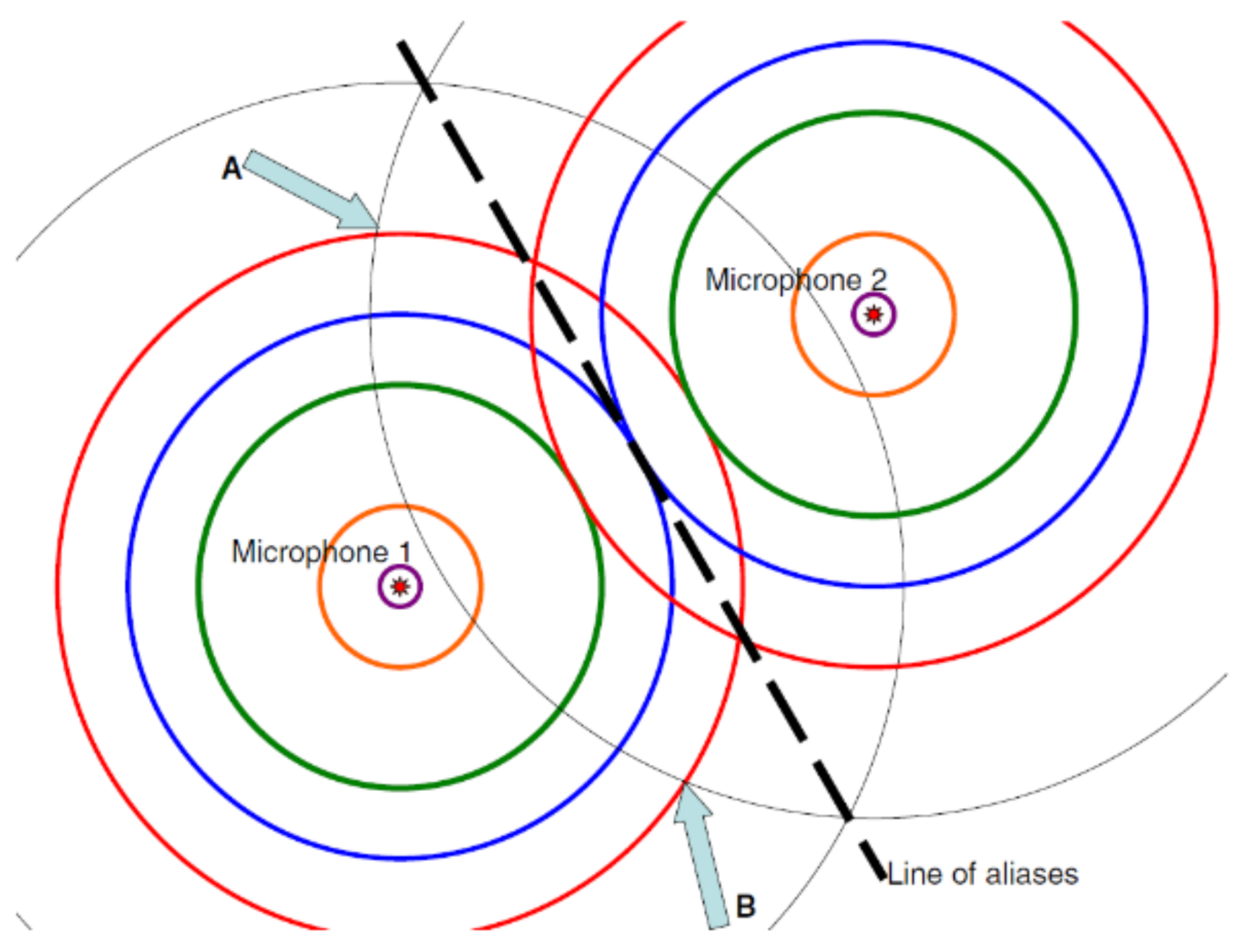
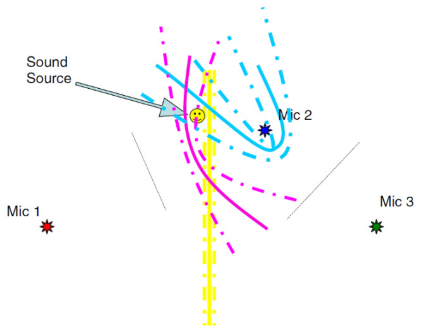
3.4.1. Geometry of the Problem

The geometry of the arrangement of microphones with the source must be carefully chosen due to the issues discussed in this section. Some confusion regarding the location of the source may arise because of aliases. This situation occurs when the number of microphones in the system is too low or when they are arranged in a manner that leads to redundancy. This issue can be resolved by adding more microphones to the system. The geometry must be considered to minimize the number of microphones in the system. This would allow us to add more microphones economically. In order to use an even smaller number of microphones, the number of source signals can also be reduced to one. Evidently, source localization cannot be achieved by using one microphone as the comparison between arrived signals at different locations cannot be carried out in this case. The use of multiple microphones require a well justified geometrical arrangement with the source. The experimental arrangement is chosen by examining the possible solutions to limit the sound source. Here, we first assumed a possible arrangement where only two microphones were present in the experiment.

In case of an arrangement of two microphones only, the source must be located on the same line where the two microphones are present. If this condition is not met, the performance of the system will decrease. In Figure 6, the scenario where the source is located on the same line that is passing through microphones A and B is demonstrated. The black line represents the plane where the two microphones and the source are placed and the points A and B represent the aliases.

In order to improve the results of the system, some constraints must be imposed on the source. In order to extend these constraints, another microphone is added to the system, which results in the total number of microphones being three. If this microphone is added to the same line that is passing through the first two microphones and the source, this arrangement would lead to redundancy. Hence, all three microphones must not be placed on the same line. We consider a case where the microphones are arranged in the shape of a triangle. The 3D coordinates of the point will then be determined where the three hyperbolas intersect. A solution to such a system may be indefinite and may not be possible to determine. Some inherent inaccuracies are associated with the source localization system, which is present due to some limitations in the sampling performed by the data acquiring system and some imprecisions in measuring the exact location of the microphones. This would lead to a case where the system will become overdetermined and inconsistent. This is demonstrated in the Figure 7. In this figure, each pair of microphones will make its own assumption about the source location. For example, according to the microphones one and three, the location of the source lies on a line that is bisecting the line segment connecting them at right angles. According to the remaining pairs of microphones, the source lies on the two hyperbolas as depicted in the figure. Hence, some optimization methods are required to be applied to the system to reach to a consistent solution. After optimization, the system will locate the source on a closed curve resembling an ellipse.

In the case of four microphones and a source, we would have a scenario identical to the one depicted in Figure 7 except for the fact that the system would be complex in terms of dimensions. The line would be replaced by a plane and, in place of hyperbolas, there will be hyperboloids. In order to avoid microphone redundancy and increased resource consumption, the microphones must be placed at the corner points of a tetrahedral. The precision of the system will be reduced if all the microphones are placed on the same plane. Hence, the best configuration of microphones is the one where all the microphones are placed at the tips of a tetrahedral shape.

3.4.2. Cross Correlation for Detection of Delays

The difference between the times at which the signal has arrived at the two microphones is referred to as the time delay of the signal. While designing the geometrical arrangement of the microphones, we made an assumption that this time delay between any pair of microphones in the system is known. This time delay can be computed using a signal processing technique referred to as cross correlation. This method takes input of the two copies of the signal received at a pair of microphones. The outputs of this function are some coefficients referred to as cross correlation coefficients, which correspond to the value of each calculated time delay. The cross-correlation coefficients are computed by taking a sum of product of the corresponding portion of the signals when they intersect with one another [65]. The value of each cross correlation coefficient represents a specific time delay of a signal in reaching the two microphones [66]. The input signals recorded at the two microphones are represented by “a” and “b” respectively. The symbol n denotes their mean, while the subscripts show the input signals. Row vectors are used to store the signals and indices are used to refer to their elements.

3.4.3. Sound Localization

The sound localization routine makes use of the geometry of the system. It also runs the cross-correlation function, which is discussed above. The routine is designed such that it can work with both real experimental data and simulated data, which is hardcoded into the system. In the simulation mode, the source sound is produced by mixing sound signals from two sources. The sound signals are two speech sounds which are combined in MATLAB by using vector additions. The features that are complex and intrusive and show the differences between real and simulated results are neglected.

The source localization function is able to take as input any amount of signals. In this case, there are four signals which are recorded in the lab through the microphone configuration. These signals can also be simulated using the MATLAB code where the predefined geometry of the system is hardcoded in the function. Each signal pair recorded by the pair of microphones is cross correlated to find the time delays between them. The product of the speed of sound, with the time delay values, represents the perceived position of the source corresponding to the microphone’s arrangement where the location of each microphone is predetermined. The major aim of the sound source localization routine is to find the 3D location (X, Y and Z) of the source with respect to this arrangement. The difference in path length has been calculated as the sound signal is received by the microphone pairs after being released by the source. The location coordinates of the source, which are to be computed, and the predetermined 3D locations of the microphones are used to express this difference. This system possesses an overdetermined nature. An inherent imprecision lies in measuring the locations of the various components of the system. Due to these factors, the variables which show the exact location coordinates may be indefinite or non-existing. This indicates the need to perform a 1D optimization in order to locate the source coordinates. This is achieved by minimization of the difference among the following two factors: (a) path length difference expressing the source coordinates and (b) a numerical value achieved as a cross correlation coefficient. In MATLAB, this optimization was performed using the Simplex scheme which is one of the standard methods being used for optimization. Other methods for optimization can also be carried out for this purpose.

4. Results

4.1. Experimental Set Up

In order to test the source localization program, experiments were conducted in a laboratory. Figure 8 displays the experimental setup to record the sound signals. The experiments were based on various sound recording procedures. A fixed 3D coordinate system was established in the laboratory to carefully measure the locations of microphones in 3D space so that they can be provided as input to the program. A tetrahedral was visualized for which the length of each side measured around 2.5 m. Each of the four microphones was arranged at the corners of this tetrahedral shape. Each microphone was then connected to a laptop executing the LabView application [67]. The four signals received by the microphones were saved into an excel spreadsheet to be used by the MATLAB function for source localization. The locations of microphones in 3D were provided as input to the program. The location of the source was carefully measured so that it can be compared with the 3D location that is calculated by our source localization routine. Multiple experiments were conducted in the laboratory using this configuration of microphones, where the sound source was placed at different positions in the lab area.

The experimental arrangement consists of two separate nodes. Each node consists of an array of two microphones. Sound signals from two sources are combined and mixed with noise to imitate the practical scenario of the sound localization problem accurately. The icaDemo() function utilizes Independent Component Analysis (ICA) to extract the source signals [68]. ICA reproduces the source signals with amplitude and order indeterminacy. This function divides a complex sound signal into separate non-Gaussian signals. As in our case, the source signal consists of the combination of multiple signals at each time component t. The result is a multivariate signal. Hence, there is a need to isolate the original or the target sound from this mixture of signals and to remove other noise or irrelevant data. Using an assumption of independence based on statistics, separation of signals using blind ICA shows good performance. Another example of the application of ICA is a problem referred to as the “cocktail party problem”. In this problem, people are talking in the room at the same time and there is a need to separate the speech signals from the recorded sound. No time delay or echoes are considered to simplify the problem.

The localization routine uses the recorded signals, the location of microphones and the sound source location to calculate the time delays between the arrival of the signals, as described in the previous section.

4.2. Implementation

In the MATLAB code implementation, the signals from the microphones were received as input to the program to visualize them and to compare the various versions of the same signal that was received by the microphones placed at different locations. An application called LabView was used to save real values from a lab experiment to an excel file which can be provided for the program. In that configuration, microphones should be hooked up to a computer, which ran a Lab View program. The program will save signals from the microphones into a spreadsheet for later processing by the MATLAB source localization routine. In that case, the arguments to localize1() MATLAB function will be the following.

$$localize1\left(0, \left[123\right]\right), address)$$

(11)

In this command, 0 indicates that real values will be provided to the program, [1 2 3] is the source matrix and the address is the location of the excel file containing the source signals recorded from microphone. To simulate the results from the signal values that are already hardcoded in the program, the following command will be used.

$$localize1\left(1, \left[1 2 3\right]\right)$$

(12)

Here, 1 signifies that simulation is required so we do not need the address of another data file. The source matrix is [1 2 3]. The source matrix given is given as input in the command and indicates the location of the source. It is used to calculate the delay in the transmission of the signal relative to the microphone configuration.

The function simDelay calculates time delay between all pairs of microphones using the distance function. It uses the locations of the microphones and the source and passes them onto the distance function to calculate a numerical value, which is used by simDelay to calculate a final delay value. This function determined the difference in path length as sound travels from the source to any pairs of microphones.

The delay value is used by localize1() to localize the sound source. It passes on this value to the ellipseMerit function, which finally localizes the sound source in 3D. These are the coordinates of the location of the sound relative to this microphones configuration. This time delay information is multiplied by the speed of sound to give information that encapsulates the conceived constellation of the source with respect to the arrays of microphones, for which the location is already known.

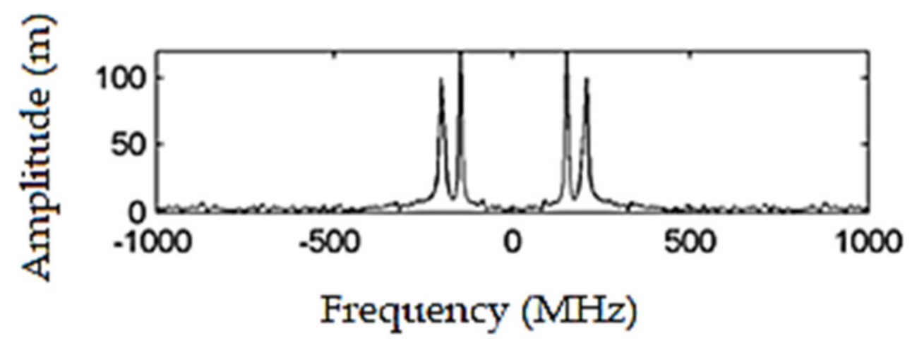
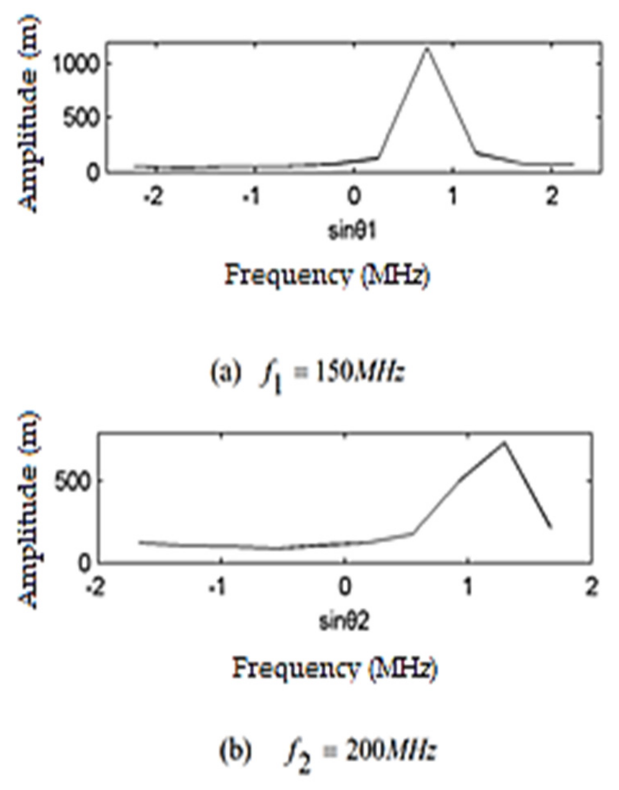
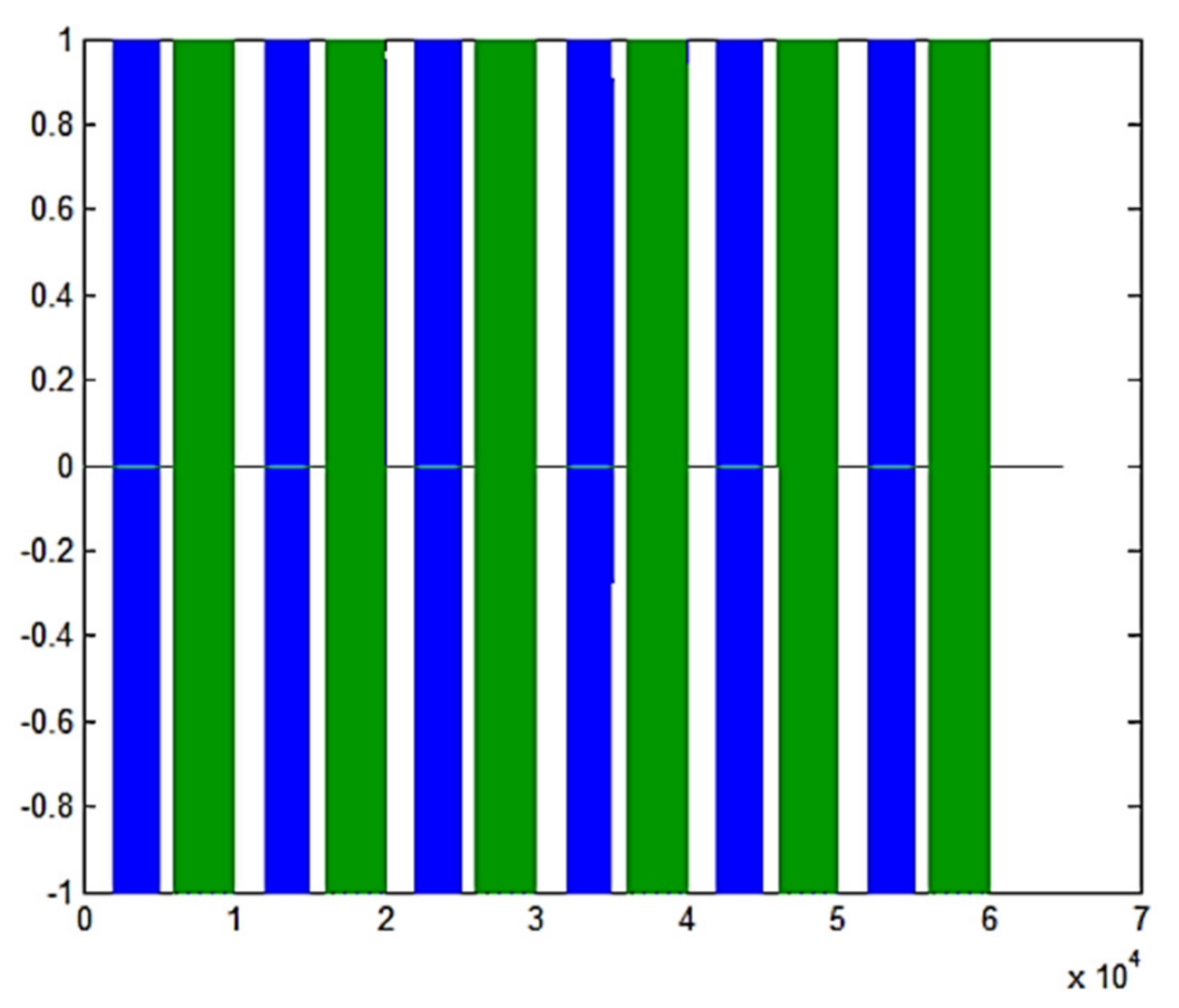
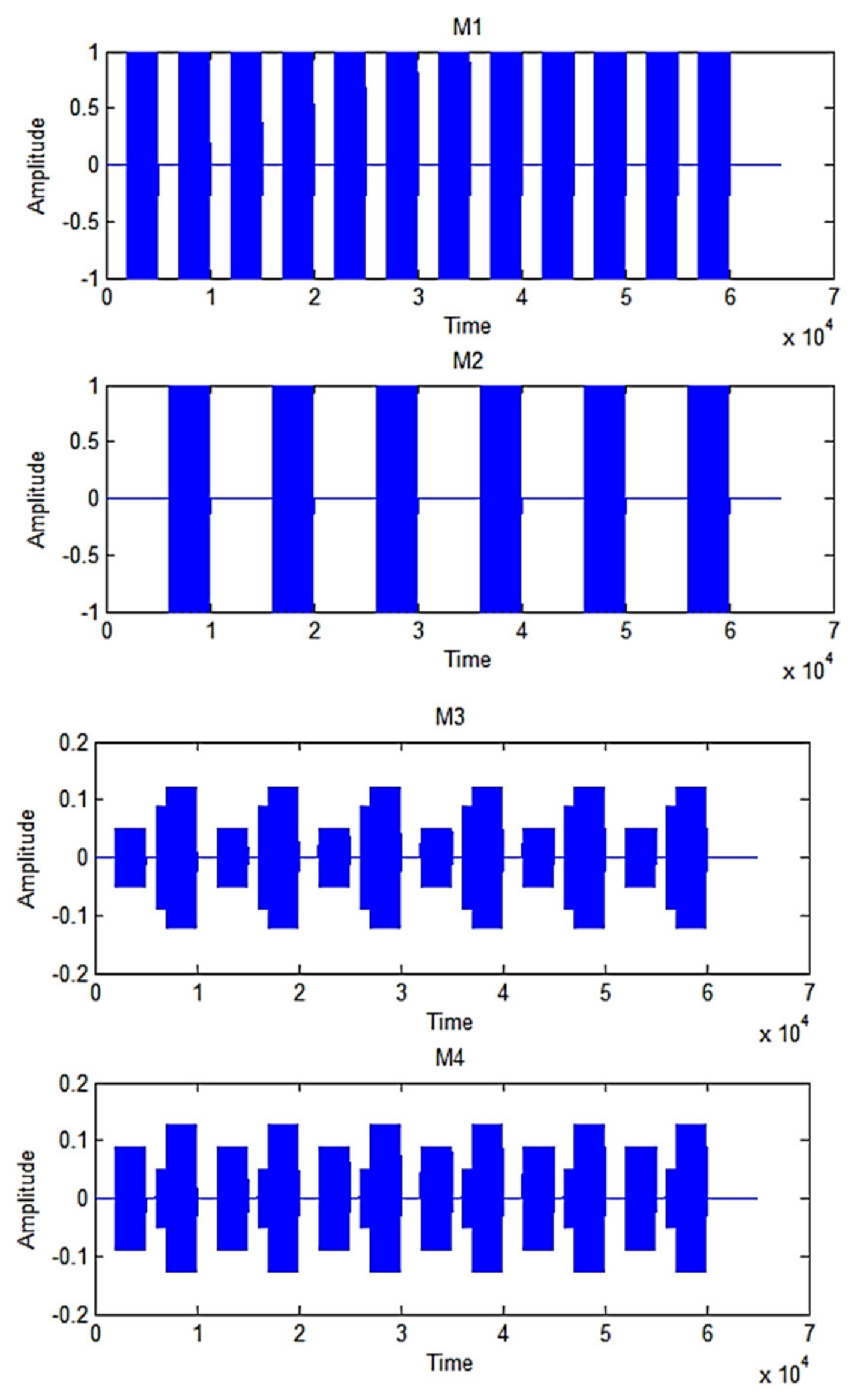
4.2.1. Developing Source Signal

The code snippet shown in Figure 9, loads a noise and two speech sound signals. These sounds are reshaped and combined into a single vector.

4.2.2. Error Factor

In order to measure the error factor corresponding to the estimated source location, we use a “condition number”. This factor is calculated by using both forward and backward errors. Forward error represents the accuracy of the determined source location. Backward error assesses how accurately the values of delay and the microphone location are known. The condition number is calculated by dividing the forward error by the backward error. The lower this number is, the lower the error factor will be in source localization. The code segment shown in Figure 10 shows how condition number is calculated.

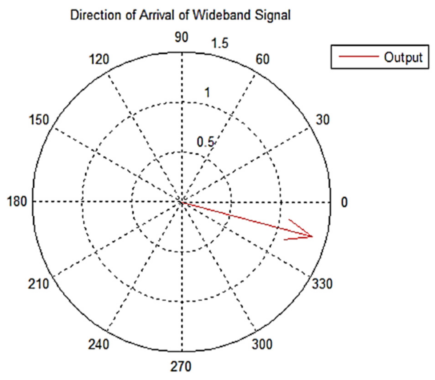
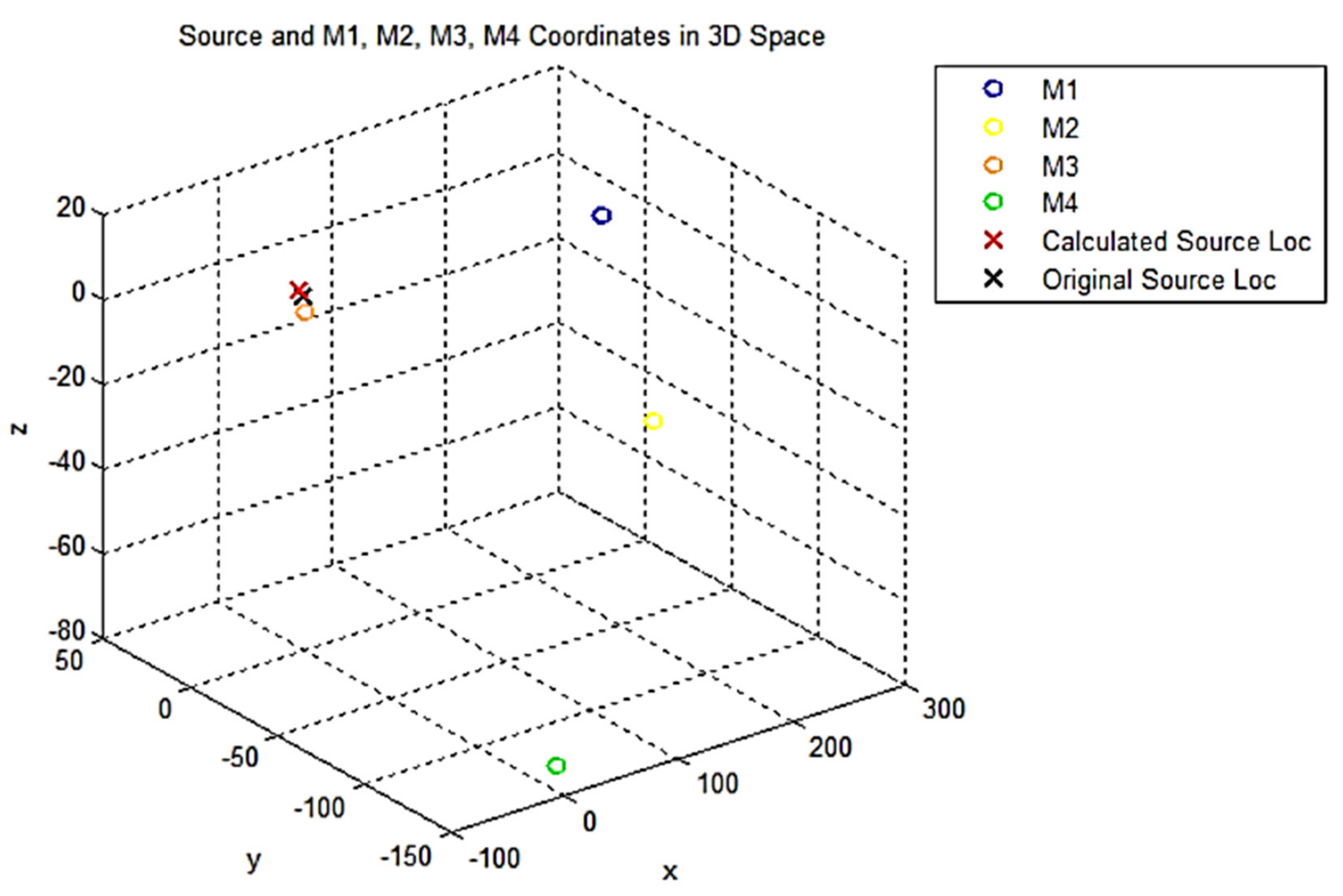
4.3. Results

In order to test the source localization function, a geometrical arrangement of microphones was set up where each of the microphones was placed at the corners of a tetrahedral and a source could be located at any place in the 3D space. The recorded signals were saved into a spreadsheet file where they could be accessed and taken as input to the source localization program. The results of the experiments clearly depicted the robustness of the source localization program. A condition number was calculated for each of the computed 3D coordinates of the source. The results showed that when the sound source was near the center of the tetrahedral, the value of this condition number was in the order of one. This indicates that if there exists a percent error in the positions of the microphones, it will be enhanced to a value possessing a magnitude of 1. This error will also affect and show up in the location coordinates of the source determined by the routine. It must be noted that there was an uncertain variation in the value of this condition number when the source was placed far from the middle of the tetrahedral. Due to the geometrical nature of the problem, the robustness of the results depend on the area where the source is located. Even a little miscalculation in the position coordinates of the microphones result in the situation where a larger area is occupied by the wider portion of the hyperbolic strips and the narrow portion sweeps a smaller area. This implies that when the source is not placed near the center of the constellation of the microphones, a little misspecification in the source position would result in the miscalculation in the location of the sound source. Another prospect for future research is the uncertain behavior of the condition number during the source localization.

The use of a minimum amount of microphones in the experiments is justified by the area specific robustness of the system. Most applications do not require the small advantage of having more microphones in the system where the source is at a region, which maintains the robustness of the system. The minimum number of microphones can only be used in the condition where the source is located within the tetrahedral shape of the microphones arrangement. This routine was tested on the data gathered from laboratory experiments and was also further tested using simulations. For lab data, condition number was in the order of ten. This error figure can be attributed to the sound disturbances in the lab such as echo and noise. These discrepancies can result in an inaccuracy in the calculation of time delay data by the cross correlation function. These issues can be resolved through the use of better tools for acquiring data and conducting the experiments in an environment where there is less reverberations. A configuration of five microphones can also be used to improve the results. However, that would result in increased resource usage, while achieving the marginal benefits. The four microphone configuration has yielded satisfactory performance in terms of robustness in our experiments.

Figure 9 shows the DOA of the source sound signal as determined through the method described previously. This angle is calculated to be approximately 75.4 degrees using this method. This angle represents the direction from which the sound wave has arrived to the microphone arrays. The direction is relative to the array of sensors. It depends on the position of the source and the microphones in the 3D space.

Figure 10 shows the original input signal reaching to the microphones. Figure 11 shows the input signals received by each of the four microphones when sample rate was set to 10,000. The amplitude vs. time graphs of the input sound signals at each microphone have been plotted. By the comparison of the graphs shown in Figure 11, we can observe that M1 has recorded a sound signal that is closest to the original one. This shows that each of the microphones has received some portion of the input sound signal. However, there are differences in the sound waves recorded by each microphone due to their individual locations and distances from the source. Due to the distance from the source and their position, each microphone receives a slightly different signal in terms of intensity, which has been depicted in these graphs. All microphones were able to receive a signal that was similar to the source sound. However, some of them received exaggerated or degraded versions of the signal due to echo, noise and related disturbances present in the laboratory environment.

In order to run the source localization routine, we typed the following command into the MATLAB command prompt: localize1 (1, [30 100 10]). Here localize1 is the name of the source localization routine. The argument, 1, passed to this routine indicates that a simulation is required using the already hardcoded data in the program. The actual coordinates of the source measured in the lab are (30, 100, 10) which are passed to the routine. The calculated coordinates were (30.0132, 100.4015, 10.0345). Similarly, the sound source locations were found at (−2, 3, 1) and (−30, −10, −100). The 3D models were generated when source was at (30, 100, 10), (−2, 3, 1) and (−30, −10, −100). Figure 12, Figure 13 and Figure 14 shows the 3D model generated by the systems at (30, 100, 10), (−2, 3, 1) and (−30, −10, −100), respectively. The plot shown in these figures compares the original source location with the calculated one. These results show that the determined location of the source is precise and has only a slight deviation from the actual source coordinates.

Table 1. Experimental results.

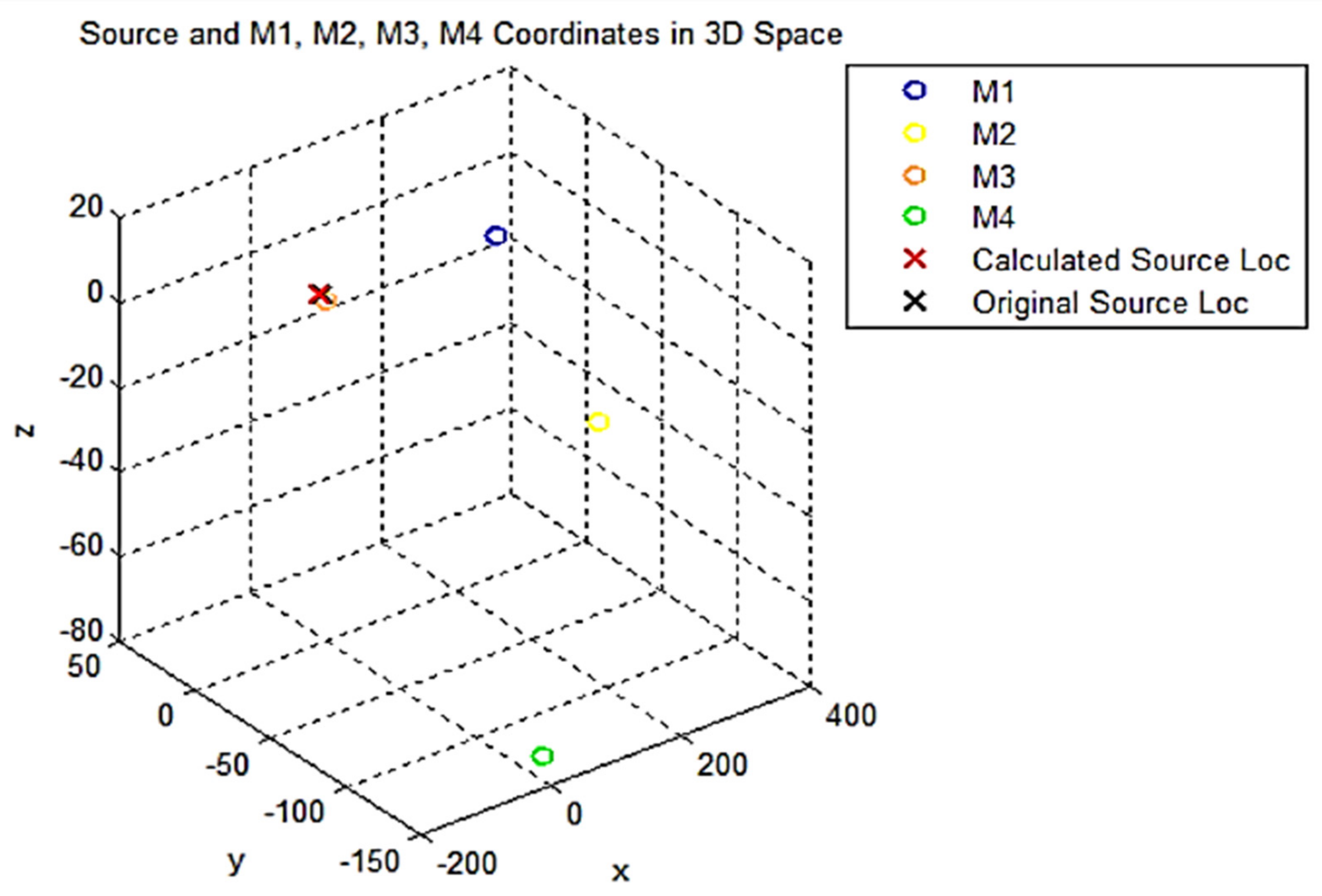
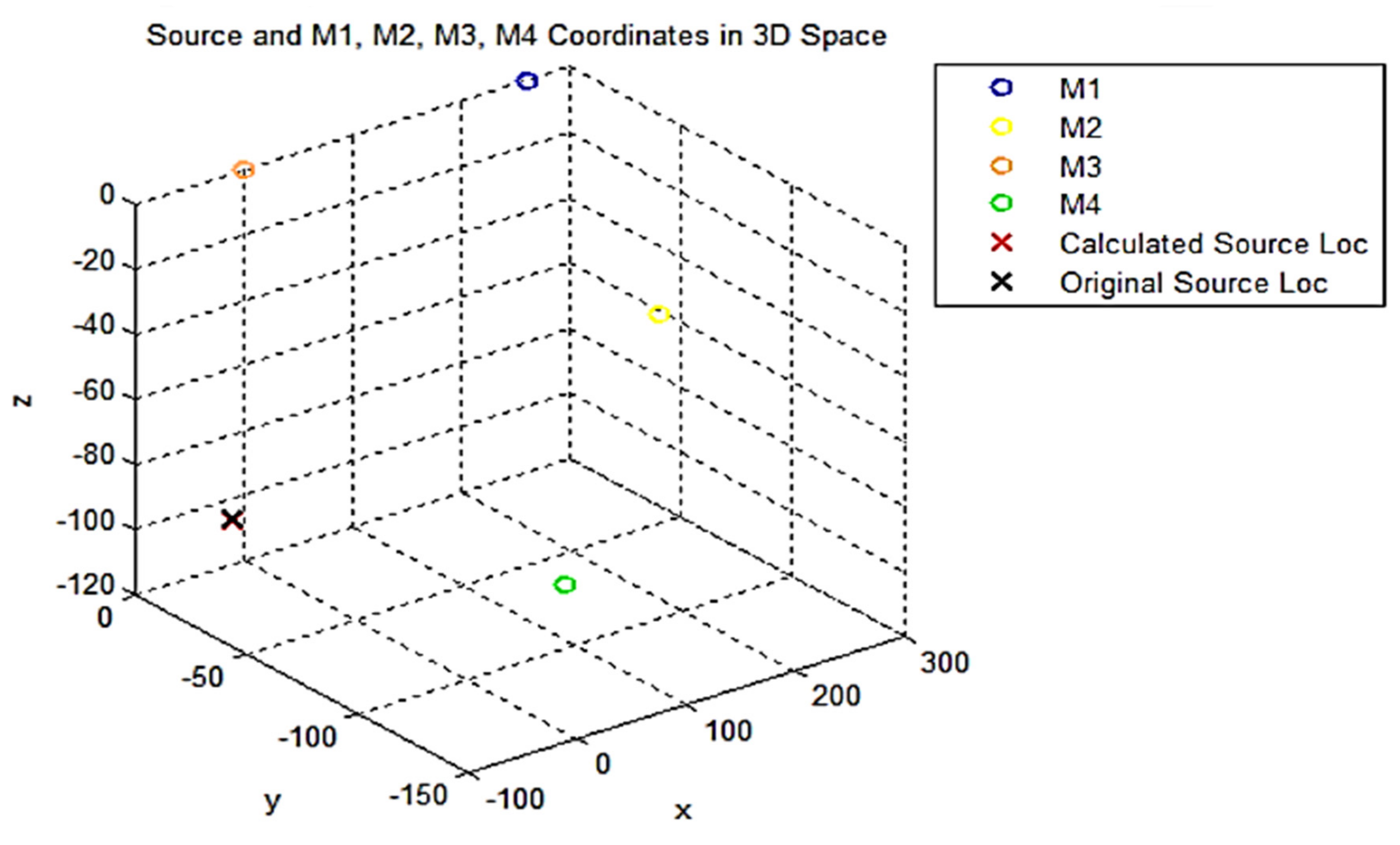
No.	Sampling Rate	Original Source Location	Calculated Source Location	DOA (Degrees)	Condition Number
1.	100	(30, 100, 10)	(30.0132, 100.4015, 10.0345)	75.4	1.2557
2.	5000	(−2, 3, 1)	(−2.1378, 3.6586, 1.1087)	50	0.999
3.	10,000	(−30, −10, −100)	(−29.7702, −9.3940, −100.8523)	45.6	0.3350
4.	50,000	(0, 1, 2)	(0.0010, 1.2150, 2.0050)	26.1	1.24

summarizes the results obtained by the series of experiments performed by taking the input of signals at different sampling rates. As shown in the results, there are little differences between the real and the calculated values of the location of the sound source at all sampling rates. The DOA is also calculated for each of the input. For each input, the corresponding condition number is also calculated by utilizing the forward and the backward error. Using the differences in actual and calculated values, the measured accuracy of sound source localization of the proposed system is found to be 96.77%. The average condition number calculated as the error factor of this system is found to be 3.8%.

4.4. Comparison of Results

In order to compare the results of this study, we review some state-of-the-art methods that have recently been proposed for the sound source localization. In order to gather such studies from recent literature, we used a set of keywords related to sound source localization. This initial set of keywords include the words: “sound localization”, “DOA”, “microphone” and “arrays”. More keywords found in the recent literature relevant to these keywords were found using the VOS Viewer software package. The obtained keywords were used to design search phrases, which are to be used in the search engine of Google Scholar. Research articles published over the past ten years were retrieved and reviewed. The state-of-the-art methods found in these articles are discussed below.

Risoud et al. worked on finding the source of sound in 3D: azimuth, height and distance. Different measures such as time difference and level difference along with a head-transfer function were utilized. The accuracy of this system highly depends on the azimuthal position of the source. For example, the uncertainty of localization is 3–4 degrees when azimuth is equal to zeros degrees [69]. Pavlidi et al. presented a source localization method for multiple sound sources. The method applies some sparsity limitations on the source sound signals. A circular arrangement is used for microphones to overcome the limitations faced by linear arrays. This method relies on computing time frequency areas for each source. The method has been proven to perform better than some other standard DOA estimations while simultaneously reducing the complexity of computation [70]. Yalta et al. used deep neural networks for sound source localization by using an array of microphones in a noise-prone environment. The accuracy of this system outperforms that of linear models. This was achieved by applying general pre-processing steps to the signals and training the model for a short period of time [71]. Tuma et al. proposed a sound source localization system based on beamforming that measures the angles of the source sound signals and the distance between them. Experimental results showed a slight difference between the calculated and actual DOA which can be attributed to sampling frequency and rounding off [72]. An extension to the Steered Response Power-Phase Transform (SRP-PHAT) method was proposed by Cobos et al. [73]. In this approach, a generalized cross correlation (GCC) was used with each microphone pair. The system was tested under varying noise and sound conditions to verify the effectiveness of the proposed method.

Table 2. Results comparison.

No.	Method	Measured Factors	No. of Microphones	Results	Ref
1.	Interaural time and level difference, head transfer function	Azimuth, elevation Distance	0	Uncertainty = 3–4 degrees	[69]
2.	Time frequency	DOA	3	Success Score = 61.62%	[70]
3.	Deep learning	DOA	7	Accuracy = 71.46%	[71]
4.	Beamforming	TDOA, Distance	3	Error = 0.11%	[72]
5.	GCC SRC-PHAT	DOA	4	RMSE = 0.31	[73]
6.	Proposed	DOA, 3D Coordinates	4	Accuracy = 96.77%, Error factor = 3.8%	-

compares the results of these approaches with the method proposed in this study. The comparative analysis show that the results of the proposed method are better or comparable to the state-of-the-art methods.

5. Discussion

Sound localization is a field of signal processing that deals with identifying the origin of a detected sound signal [74,75,76,77,78,79]. This involves determining the direction and distance of the source of the sound. Some useful applications of this phenomenon exists in speech enhancement, communication, radars and in the medical field as well. The experimental arrangement requires the use of microphone arrays, which records the sound signal. Some methods involve using ad-hoc arrays of microphones because of their demonstrated advantages over other arrays. In this research project, the existing sound localization methods have been explored to analyze the pros and cons of each method [80,81,82,83,84,89,90,91,92]. A novel sound localization routine has been formulated, which uses both DOA of sound signals along with location estimation in three-dimensional space to precisely locate a sound source as mentioned in Appendix A. The experimental arrangement consists of four microphones and a single sound source. Previously, sound source has been localized using six or more microphones. The precision of sound localization has been demonstrated to increase with the use of more microphones. In this research, however, we minimized the use of microphones to reduce the complexity of the algorithm and the computation time. The method brings novelty in the field of sound source localization by utilizing less resources and by providing results that are on par with the more complex methods that require more microphones and additional tools to locate the sound source.

Sound localization for microphones provide a great potential for the future advancements in this field. Many different methods have been used for this purpose that rendered many useful applications. This document presents a brief overview of some already used method for the sound localization process along with a comparison of their features, which present their strengths and weaknesses in a better manner. After studying different methods of SSL, DOA is selected for the task of sound source localization using microphone arrays. DOA has some useful features such as the elimination of the need for synchronization and low bandwidth usage, which renders it better than other methods for localization. Methods of DOA can be implemented by many different algorithms depending on the application. These algorithms are also studied and, out of them, a phase difference based method is chosen.

Detailed explanation of the DOA by using the phase difference based method is given in the document. The concept of sound localization with the DOA technique using a lesser number of nodes is the basic part of the project. In order to extend the method of DOA to utilizing two or three number of nodes, the method is first studied on four nodes. Discussions of some of the problems which can occur during the implementation of the same concept on a different number of nodes are examined. Framework for the process of using only two nodes was presented, which does not compromise on the accuracy and efficiency of the result. Each node has two microphones, which renders the total number of microphones as four. The system has demonstrated an accuracy of 96.77% with an error factor of 3.8%.

6. Conclusions

This study presents novel methods for determining DOA of the source signal and its 3D coordinates. The 3D coordinates of the source are determined using phase differences between input signals recorded by the microphones. The system reduces the number of microphones used in the system by limiting the number of microphones to four. The microphones are arranged such that they form two separate nodes. This arrangement is beneficial in that the resulting sound source localization method can be used in hearing aids and related devices. The system is also designed to work under reverberant environments. The results show that the system generates an accuracy of 96.77% with a recorded error rate of 3.8%.

In the future, the sound source localization system can be made more compact by further reducing the number of microphones. The existing error factor in the results can be reduced by decreasing the noise content mixed with the source signal. Further improvement can be performed by devising a novel geometrical arrangement for the microphones, which can yield better accuracy. More challenges in the domain of sound source localization can be tackled by exploring deep learning methods, which requires training data but can also offer promising results in terms of accuracy. Further work can be performed in classifying the localized sound sources.

References

- Wu, K.; Khong, A.W. Sound Source Localization and Tracking. In Context Aware Human-Robot and Human-Agent Interaction; Springer: Cham, Switzerland, 2016; pp. 55–78. [Google Scholar]
- Alameda-Pineda, X.; Horaud, R. A Geometric Approach to Sound Source Localization from Time-Delay Estimates. IEEE/ACM Trans. Audio Speech Lang. Process. 2014, 2, 1082–1095. [Google Scholar] [CrossRef] [Green Version]
- Burges, S.; Kuang, Y.; Astroom, K. TOA sensor network self-callibration for receiver and transmitter spaces with difference in dimensions. Signal Process. 2015, 107, 33–42. [Google Scholar] [CrossRef] [Green Version]
- Chen, M.; Liu, Z.; He, L.-W.; Chou, P.; Zhang, Z. Energy-Based Position Estimation of Microphones and Speakers for Ad Hoc Microphone Arrays. In 2007 IEEE Workshop on Applications of Signal Processing to Audio and Acoustics; Institute of Electrical and Electronics Engineers (IEEE): New York, NY, USA, 2007; pp. 22–25. [Google Scholar]
- Sheng, X.; Hu, Y.H. Energy Based Acoustic Source Localization. In Information Processing in Sensor Networks; Lecture Notes in Computer Science; Springer: Berlin, Germany, 2003; Volume 2634, pp. 285–300. [Google Scholar]
- Kundu, T. Acoustic source localization. Ultrasonics 2014, 54, 25–38. [Google Scholar] [CrossRef]
- Aston, J. Sound Localization and New Applications of Its Research; Stephen, F., Ed.; Applied Perception Projects and Service-Learning Project; Austin State University: Nacogdoches, TX, USA, 2003. [Google Scholar]
- Choi, H.; Choi, H.; Park, J.; Park, J.; Lim, W.; Lim, W.; Yang, Y.-M.; Yang, Y.-M.; Choi, H.; Choi, H.; et al. Active-beacon-based driver sound separation system for autonomous vehicle applications. Appl. Acoust. 2021, 171, 107549. [Google Scholar] [CrossRef]
- Sakanashi, R.; Ono, N.; Miyabe, S.; Yamada, T.; Makino, S. Speech enhancement with ad-hoc microphone array using single source activity. In Proceedings of the 2013 Asia-Pacific Signal and Information Processing Association Annual Summit and Conference, Kaohsiung, Taiwan, 29 October–1 November 2013; pp. 1–6. [Google Scholar]
- Hennecke, M.H.; Fink, G.A. Towards acoustic self-localization of ad hoc smartphone arrays. In Proceedings of the 2011 Joint Workshop on Hands-Free Speech Communication and Microphone Arrays, Edinburgh, Scotland, 30 May–1 June 2001. [Google Scholar]
- Lienhart, R.; Kozintsev, I.; Wehr, S.; Yeung, M. On the importance of exact synchronization for distributed audio processing. In Proceedings of the IEEE International Conference on Acoustics, Speech, and Signal Processing, Hong Kong, China, 6–10 April 2003. [Google Scholar]
- Hassani, A.; Bertrand, A.; Moneen, M. Cooperative integrated noise reduction and node-specific direction-of-arrival estimation in a fully connected wireless acoustic sensor network. Signal Process. 2015, 107, 68–81. [Google Scholar] [CrossRef] [Green Version]
- Munawar, H.S.; Khan, S.I.; Anum, N.; Qadir, Z.; Kouzani, A.Z.; Parvez Mahmud, M.A. Post-Flood Risk Management and Resilience Building Practices: A Case Study. Appl. Sci. 2021, 11, 4823. [Google Scholar] [CrossRef]
- Yost, W.A.; Zhong, X. Sound source localization identification accuracy: Bandwidth dependencies. J. Acoust. Soc. Am. 2014, 136, 2737–2746. [Google Scholar] [CrossRef]
- Rascon, C.; Meza, I. Localization of sound sources in robotics: A review. Robot. Auton. Syst. 2017, 96, 184–210. [Google Scholar] [CrossRef]
- Song, T.; Chen, J.; Zhang, D.B.; Qu, T.S.; Wu, X.H. Sound source localization algorithm using microphone array with rigid body. In Proceedings of the 22nd International Congress on Acoustics, Buenos Aires, Argentina, 5–9 September 2016. [Google Scholar]
- Seco, F.; Jiménez, A.R.; Prieto, C.; Roa, J.; Koutsou, K. A survey of mathematical methods for indoor localization. In Proceedings of the 2009 IEEE International Symposium on Intelligent Signal Processing, Budapest, Hungary, 26–28 August 2009; pp. 9–14. [Google Scholar]
- Pertilä, P. Acoustic Source Localization in a Room Environment and at Moderate Distances; Tampere University of Technology: Tampere, Finland, 2009. [Google Scholar]
- Chen, J.; Benesty, J.; Huang, Y. Time delay estimation in room acoustic environments: An overview. EURASIP J. Adv. Signal Process. 2006. [Google Scholar] [CrossRef] [Green Version]
- Liu, R.; Wang, Y. Azimuthal source localization using interaural coherence in a robotic dog: Modeling and application. Robotica 2010, 28, 1013–1020. [Google Scholar] [CrossRef]
- Mandel, M.I.; Ellis, D.P.; Jebara, T. An em algorithm for localizing multiple sound: Sources in reverberant environments. In Proceedings of the Twentieth Annual Conference on Neural Information Processing Systems, Vancouver, BC, Canada, 4–7 December 2006. [Google Scholar]
- Viste, H.; Evangelista, G. On the use of spatial cues to improve binaural source separation. In Proceedings of the 6th International Conference on Digital Audio Effects (DAFx-03), London, UK, 8–11 September 2003; pp. 209–213. [Google Scholar]
- Woodruff, J.; Wang, D. Binaural Localization of Multiple Sources in Reverberant and Noisy Environments. IEEE Trans. Audio Speech Lang. Process. 2012, 20, 1503–1512. [Google Scholar] [CrossRef]
- Kulaib, A.R.; Al-Mualla, M.; Vernon, D. 2D Binaural Sound Localization: For Urban Search and Rescue Robotics. In Mobile Robotics; World Scientific: Singapore, 2009; pp. 423–435. [Google Scholar]
- Deleforge, A.; Horaud, R. 2D sound-source localization on the binaural manifold. In Proceedings of the 2012 IEEE International Workshop on Machine Learning for Signal Processing, Santander, Spain, 23–26 September 2006; pp. 1–6. [Google Scholar]
- Keyrouz, F.; Diepold, K. An enhanced binaural 3D sound localization algorithm. In Proceedings of the 2006 IEEE International Symposium on Signal Processing and Information Technology, Vancouver, BC, Canada, 27–30 August 2006; pp. 662–665. [Google Scholar]
- Keyrouz, F.; Diepold, K.; Keyrouz, S. Humanoid binaural sound tracking using Kalman filtering and HRTFs. In Robot Motion and Control; Springer: London, UK, 2007; pp. 329–340. [Google Scholar]
- Shaukat, M.A.; Shaukat, H.R.; Qadir, Z.; Munawar, H.S.; Kouzani, A.Z.; Mahmud, M.A.P. Cluster Analysis and Model Comparison Using Smart Meter Data. Sensors 2021, 21, 3157. [Google Scholar] [CrossRef] [PubMed]
- Chen, J.C.; Yao, K.; Hudson, R.E. Acoustic Source Localization and Beamforming: Theory and Practice. EURASIP J. Adv. Signal Process. 2003, 2003, 926837. [Google Scholar] [CrossRef] [Green Version]
- Sheng, X.; Hu, Y.-H. Maximum likelihood multiple-source localization using acoustic energy measurements with wireless sensor networks. IEEE Trans. Signal Process. 2005, 53, 44–53. [Google Scholar] [CrossRef] [Green Version]
- So, H.C.; Chan, Y.T.; Chan, F.K.W. Closed-Form Formulae for Time-Difference-of-Arrival Estimation. IEEE Trans. Signal Process. 2008, 56, 2614–2620. [Google Scholar] [CrossRef] [Green Version]
- Urruela, A.; Riba, J. Novel closed-form ML position estimator for hyperbolic location. In Proceedings of the 2004 IEEE International Conference on Acoustics, Speech, and Signal Processing, Montreal, QC, Canada, 17–21 May 2004; Volume 2, p. ii-149. [Google Scholar]
- Strobel, N.; Rabenstein, R. Classification of time delay estimates for robust speaker localization. In Proceedings of the 1999 IEEE International Conference on Acoustics, Speech, and Signal Processing, Phoenix, AZ, USA, 15–19 March 1999; Volume 6, pp. 3081–3084. [Google Scholar]
- Zhang, C.; Zhang, Z.; Florêncio, D. Maximum likelihood sound source localization for multiple directional microphones. In Proceedings of the 2007 IEEE International Conference on Acoustics, Speech and Signal Processing-ICASSP’07, Honolulu, HI, USA, 15–20 April 2007; Volume 1, p. I-125. [Google Scholar]
- Zhang, C.; Florencio, D.; Ba, D.E.; Zhang, Z. Maximum Likelihood Sound Source Localization and Beamforming for Directional Microphone Arrays in Distributed Meetings. IEEE Trans. Multimed. 2008, 10, 538–548. [Google Scholar] [CrossRef]
- Smith, J.; Abel, J. Closed-form least-squares source location estimation from range-difference measurements. IEEE Trans. Acoust. Speech Signal Process. 1987, 35, 1661–1669. [Google Scholar] [CrossRef]
- Brandstein, M.; Adcock, J.; Silverman, H. A closed-form location estimator for use with room environment microphone arrays. IEEE Trans. Speech Audio Process. 1997, 5, 45–50. [Google Scholar] [CrossRef]
- Brandstein, M.S.; Silverman, H.F. A practical methodology for speech source localization with microphone arrays. Comput. Speech Lang. 1997, 11, 91–126. [Google Scholar] [CrossRef] [Green Version]
- Friedlander, B. A passive localization algorithm and its accuracy analysis. IEEE J. Ocean. Eng. 1987, 12, 234–245. [Google Scholar] [CrossRef]
- Huang, Y.; Benesty, J.; Elko, G.W.; Mersereati, R.M. Real-time passive source localization: A practical linear-correction least-squares approach. IEEE Trans. Speech Audio Process. 2001, 9, 943–956. [Google Scholar] [CrossRef]
- Canclini, A.; Antonacci, F.; Sarti, A.; Tubaro, S. Acoustic source localization with distributed asynchronous microphone networks. IEEE Trans. Audio Speech Lang. Process. 2012, 21, 439–443. [Google Scholar] [CrossRef]
- Omologo, M.; Svaizer, P.; Brutti, A.; Cristoforetti, L. Speaker localization in CHIL lectures: Evaluation criteria and results. In International Workshop on Machine Learning for Multimodal Interaction; Springer: Berlin, Germany, 2015; pp. 476–487. [Google Scholar]
- Mori, R.D. Spoken Dialogues with Computers; Academic Press, Inc.: Cambridge, MA, USA, 1997. [Google Scholar]
- Brutti, A.; Omologo, M.; Svaizer, P. Oriented global coherence field for the estimation of the head orientation in smart rooms equipped with distributed microphone arrays. In Proceedings of the Ninth European Conference on Speech Communication and Technology, Lisboa, Portugal, 4–8 September 2005. [Google Scholar]
- Brutti, A.; Omologo, M.; Svaizer, P. Speaker localization based on oriented global coherence field. In Proceedings of the Ninth International Conference on Spoken Language Processing, Pittsburgh, PA, USA, 17–21 September 2006. [Google Scholar]
- Padois, T.; Berry, A. Two and three-dimensional sound source localization with beamforming and several deconvolution techniques. Acta Acust. United Acust. 2017, 103, 392–400. [Google Scholar] [CrossRef]
- Lehmann, E.A.; Johansson, A.M. Prediction of energy decay in room impulse responses simulated with an image-source model. J. Acoust. Soc. Am. 2008, 124, 269–277. [Google Scholar] [CrossRef] [Green Version]
- Leyffer, S. Integrating SQP and branch-and-bound for mixed integer nonlinear programming. Comput. Optim. Appl. 2001, 18, 295–309. [Google Scholar] [CrossRef]
- Li, Z.; Duraiswami, R. A robust and self-reconfigurable design of spherical microphone array for multi-resolution beamforming. In Proceedings of the IEEE International Conference on Acoustics, Speech, and Signal Processing, Philadelphia, PA, USA, 23–23 March 2005; Volume 4, p. iv-1137. [Google Scholar]
- Lim, J.S.; Pang, H.S. Time delay estimation method based on canonical correlation analysis. Circuits Syst. Signal Process. 2013, 32, 2527–2538. [Google Scholar] [CrossRef]
- Qadir, Z.; Ever, E.; Batunlu, C. Use of Neural Network Based Prediction Algorithms for Powering Up Smart Portable Accessories. Neural Process. Lett. 2021, 53, 721–756. [Google Scholar] [CrossRef]
- Ferguson, E.L.; Williams, S.B.; Jin, C.T. Sound source localization in a multipath environment using convolutional neural networks. In Proceedings of the 2018 IEEE International Conference on Acoustics, Speech and Signal Processing (ICASSP), Calgary, AB, Canada, 15–20 April 2018; pp. 2386–2390. [Google Scholar]
- An, I.; Son, M.; Manocha, D.; Yoon, S.E. Reflection-aware sound source localization. In Proceedings of the 2018 IEEE International Conference on Robotics and Automation (ICRA), Brisbane, Australia, 21–26 May 2018; pp. 66–73. [Google Scholar]
- Grondin, F.; Michaud, F. Lightweight and optimized sound source localization and tracking methods for open and closed microphone array configurations. Robot. Auton. Syst. 2019, 113, 63–80. [Google Scholar] [CrossRef] [Green Version]
- Opochinsky, R.; Laufer-Goldshtein, B.; Gannot, S.; Chechik, G. Deep ranking-based sound source localization. In Proceedings of the 2019 IEEE Workshop on Applications of Signal Processing to Audio and Acoustics (WASPAA), New Paltz, NY, USA, 20–23 October 2019; pp. 283–287. [Google Scholar]
- Evers, C.; Löllmann, H.W.; Mellmann, H.; Schmidt, A.; Barfuss, H.; Naylor, P.A.; Kellermann, W. The LOCATA challenge: Acoustic source localization and tracking. IEEE/ACM Trans. Audio Speech Lang. Process. 2020, 28, 1620–1643. [Google Scholar] [CrossRef]
- Johnson, D.H.; Dudgeon, D.E. Array Signal Processing, Concepts and Techniques; Prentice Hall: Englewood Cliffs, NJ, USA, 1993; ISBN 978-0130485137. [Google Scholar]
- Leclère, Q.; Pereira, A.; Bailly, C.; Antoni, J.; Picard, C. A unified formalism for acoustic imaging based on microphone array measurements. Int. J. Aeroacoust. 2017, 16, 431–456. [Google Scholar] [CrossRef] [Green Version]
- Van Veen, B.; Buckley, K. Beamforming: A versatile approach to spatial filtering. IEEE ASSP Mag. 1988, 5, 4–24. [Google Scholar] [CrossRef]
- Merino-Martínez, R.; Sijtsma, P.; Snellen, M.; Ahlefeldt, T.; Antoni, J.; Bahr, C.J.; Blacodon, D.; Ernst, D.; Finez, A.; Funke, S.; et al. A review of acoustic imaging methods using phased microphone arrays. CEAS Aeronaut. J. 2019, 10, 197–230. [Google Scholar] [CrossRef] [Green Version]
- Cobos, M.; Antonacci, F.; Alexandridis, A.; Mouchtaris, A.; Lee, B. A Survey of Sound Source Localization Methods in Wireless Acoustic Sensor Networks. Wirel. Commun. Mob. Comput. 2017, 2017, 1–24. [Google Scholar] [CrossRef]
- Stoica, P.; Sharman, K.C. Maximum likelihood methods for direction-of-arrival estimation. IEEE Trans. Acoust. Speech Signal Process. 1990, 38, 1132–1143. [Google Scholar] [CrossRef]
- Xiong, B.; Li, G.; Lu, C. DOA Estimation Based on Phase-difference. In Proceedings of the 2006 8th International Conference on Signal Processing, ICSP, Guilin, China, 16–20 November 2006. [Google Scholar]
- Biniyam, T.T. Sound Source Localization and Separation; Macalester College: St. Paul, MN, USA, 2006. [Google Scholar]
- Jin, J.; Jin, S.; Lee, S.; Kim, H.; Choi, J.; Kim, M.; Jeon, J. Real-time Sound Localization Using Generalized Cross Correlation Based on 0.13 m CMOS Process. JSTS J. Semicond. Technol. Sci. 2014, 14, 175–183. [Google Scholar] [CrossRef]
- Jeffrey, T. LabVIEW for Everyone: Graphical Programming Made Easy and Fun, 3rd ed.; Kring, J., Ed.; Prentice Hall: Upper Saddle River, NJ, USA, 2006; ISBN 0131856723. [Google Scholar]
- Comon, P.; Jutten, C. Handbook of Blind Source Separation, Independent Component Analysis and Applications; Academic Press: Oxford, UK, 2010; ISBN 978-0-12-374726-6. [Google Scholar]
- Risoud, M.; Hanson, J.-N.; Gauvrit, F.; Renard, C.; Lemesre, P.-E.; Bonne, N.-X.; Vincent, C. Sound source localization. Eur. Ann. Otorhinolaryngol. Head Neck Dis. 2018, 135, 259–264. [Google Scholar] [CrossRef]
- Pavlidi, D.; Griffin, A.; Puigt, M.; Mouchtaris, A. Real-Time Multiple Sound Source Localization and Counting Using a Circular Microphone Array. IEEE Trans. Audio Speech Lang. Process. 2013, 21, 2193–2206. [Google Scholar] [CrossRef] [Green Version]
- Yalta, N.; Nakadai, K.; Ogata, T. Sound Source Localization Using Deep Learning Models. J. Robot. Mechatron. 2017, 29, 37–48. [Google Scholar] [CrossRef]
- Tuma, J.; Janecka, P.; Vala, M.; Richter, L. Sound source localization. In Proceedings of the 13th International Carpathian Control Conference (ICCC), High Tatras, Slovakia, 28–31 May 2012; pp. 740–743. [Google Scholar]
- Cobos, M.; Marti, A.; Lopez, J.J. A Modified SRP-PHAT Functional for Robust Real-Time Sound Source Localization with Scalable Spatial Sampling. IEEE Signal Process. Lett. 2010, 18, 71–74. [Google Scholar] [CrossRef]
- Zhao, S.; Ahmed, S.; Liang, Y.; Rupnow, K.; Chen, D.; Jones, D.L. A real-time 3D sound localization system with miniature microphone array for virtual reality. In Proceedings of the 2012 7th IEEE Conference on Industrial Electronics and Applications (ICIEA), Singapore, 18–20 July 2012; pp. 1853–1857. [Google Scholar] [CrossRef]
- Khan, S.I.; Qadir, Z.; Munawar, H.S.; Nayak, S.R.; Budati, A.K.; Verma, K.D.; Prakash, D. UAVs path planning architecture for effective medical emergency response in future networks. Phys. Commun. 2021, 47, 101337. [Google Scholar] [CrossRef]
- Munawar, H.S. Concepts, Methodologies and Applications. Flood Disaster Management: Risks, Technologies, and Future Directions. In Machine Vision Inspection Systems: Image Processing, Concepts, Methodologies and Applications; John Wiley & Sons, Inc.: Hoboken, NJ, USA, 2020; Volume 1, pp. 115–146. [Google Scholar]
- Munawar, H.S. Concepts, Methodologies and Applications. Image and Video Processing for Defect Detection in Key Infrastructure. In Machine Vision Inspection Systems: Image Processing, Concepts, Methodologies and Applications; John Wiley & Sons, Inc.: Hoboken, NJ, USA, 2020; Volume 1, pp. 159–177. [Google Scholar]
- Munawar, H.S.; Awan, A.A.; Khalid, U.; Munawar, S.; Maqsood, A. Revolutionizing Telemedicine by Instilling, H. 265. Int. J. Image Graph. Signal Process. 2017, 9, 20–27. [Google Scholar] [CrossRef] [Green Version]
- Munawar, H.S.; Hammad, A.; Ullah, F.; Ali, T.H. After the flood: A novel application of image processing and machine learning for post-flood disaster management. In Proceedings of the 2nd International Conference on Sustainable Development in Civil Engineering (ICSDC 2019), Jamshoro, Pakistan, 5–7 December 2019; pp. 5–7. [Google Scholar]
- Munawar, H.S. An Overview of Reconfigurable Antennas for Wireless Body Area Networks and Possible Future Prospects. Int. J. Wirel. Microw. Technol. 2020, 10, 1–8. [Google Scholar] [CrossRef] [Green Version]
- Munawar, H.S. Reconfigurable Origami Antennas: A Review of the Existing Technology and its Future Prospects. Int. J. Wirel. Microw. Technol. 2020, 10, 34–38. [Google Scholar] [CrossRef]
- Munawar, H.S.; Maqsood, A. Isotropic Surround Suppression based Linear Target Detection using Hough Transform. Int. J. Adv. Appl. Sci. 2017. [Google Scholar] [CrossRef]
- Munawar, H.S.; Khalid, U.; Jilani, R.; Maqsood, A. Version Management by Time Based Approach in Modern Era. Int. J. Educ. Manag. Eng. 2017, 7, 13–22. [Google Scholar] [CrossRef] [Green Version]
- Munawar, H.S.; Qayyum, S.; Ullah, F.; Sepasgozar, S. Big Data and Its Applications in Smart Real Estate and the Disaster Management Life Cycle: A Systematic Analysis. Big Data Cogn. Comput. 2020, 4, 4. [Google Scholar] [CrossRef] [Green Version]
- Munawar, H.S.; Zhang, J.; Li, H.; Mo, D.; Chang, L. Mining multispectral aerial images for automatic detection of strategic bridge locations for disaster relief missions. In Proceedings of the Pacific-Asia Conference on Knowledge Discovery and Data Mining, Macau, China, 14–17 April 2019; Springer: Cham, Switzerland, 2019; pp. 189–200. [Google Scholar]
- Physics@UNSW. Chapter 6: Quantifying Sound. Physclips, 2021. Available online: https://www.animations.physics.unsw.edu.au/waves-sound/quantifying/ (accessed on 18 January 2021).
- Sijtsma, P.; Stoker, R. Determination of absolute contributions of aircraft noise components using fly-over array measurements. In Proceedings of the 10th AIAA/CEAS Aeroacoustics Conference, Manchester, UK, 10–12 May 2004; p. 2958. [Google Scholar]
- Sijtsma, P. Phased array beamforming applied to wind tunnel and fly-over tests. In Proceedings of the SAE Brasil International Noise and Vibration Congress, Florianópolis, Brazil, 17–19 October 2010. [Google Scholar]
- Merino-Martínez, R.; Sijtsma, P.; Carpio, A.R.; Zamponi, R.; Luesutthiviboon, S.; Malgoezar, A.M.; Snellen, M.; Schram, C.; Simons, D.G. Integration methods for distributed sound sources. Int. J. Aeroacoustics 2019, 18, 444–469. [Google Scholar] [CrossRef]
- Qadir, Z.; Al-Turjman, F.; Khan, M.A.; Nesimoglu, T. ZIGBEE Based Time and Energy Efficient Smart Parking System Using IOT. In Proceedings of the 2018 18th Mediterranean Microwave Symposium (MMS), Istanbul, Turkey, 31 October–2 November 2018; pp. 295–298. [Google Scholar] [CrossRef]
- Qadir, Z.; Tafadzwa, V.; Rashid, H.; Batunlu, C. Smart Solar Micro-Grid Using ZigBee and Related Security Challenges. In Proceedings of the 2018 18th Mediterranean Microwave Symposium (MMS), Istanbul, Turkey, 31 October–2 November 2018; pp. 299–302. [Google Scholar] [CrossRef]
- Qadir, Z.; Ullah, F.; Munawar, H.S.; Al-Turjman, F. Addressing disasters in smart cities through UAVs path planning and 5G communications: A systematic review. Comput. Commun. 2021, 168, 114–135. [Google Scholar] [CrossRef]
- Qadir, Z.; Khan, S.I.; Khalaji, E.; Munawar, H.S.; Al-Turjman, F.; Mahmud, M.P.; Kouzani, A.Z.; Le, K. Predicting the energy output of hybrid PV–wind renewable energy system using feature selection technique for smart grids. Energy Rep. 2021. [Google Scholar] [CrossRef]