Article

Does Investor Sentiment Affect Clean Energy Stock? Evidence from TVP-VAR-Based Connectedness Approach

Graduate School of Economics, Kobe University, 2-1, Rokkodai, Nada-Ku, Kobe 657-8501, Japan
*
Author to whom correspondence should be addressed.
Energies 2021, 14(12), 3442; https://doi.org/10.3390/en14123442
Submission received: 13 May 2021 / Revised: 4 June 2021 / Accepted: 8 June 2021 / Published: 10 June 2021
(This article belongs to the Special Issue Energy Economic Analysis: Energy Transition and Sustainability)

Abstract

:
We investigated the connectedness of the returns and volatility of clean energy stock, technology stock, crude oil, natural gas, and investor sentiment based on the time-varying parameter vector autoregressive (TVP-VAR) connectedness approach. The empirical results indicate that the average total connectedness is higher in the volatility system than in the return system. The investor sentiment has a weak impact on clean energy stock. Our results show that the dynamic total connectedness across assets in the system varies with time. Furthermore, the dynamic total connectedness increases significantly during financial turmoil. Dynamic total volatility connectedness is more sensitive to financial turmoil. By comparing the connectedness estimated by the TVP-VAR model with the rolling-window VAR model, we find the dynamic total return connectedness of the TVP-VAR model is similar to the estimated results of a 200 day rolling-window VAR model.

Graphical Abstract

1. Introduction

With the deepening of the sustainable development concept, the clean energy industry has proliferated in recent years. Given the rapid expansion of the clean energy industry, the performance of the clean energy industry in financial markets has attracted increased attention from policymakers and investors. Most investors are interested in considering clean energy stock in their asset allocation to obtain investment returns and moderate risks. Therefore, it is essential to understand the interaction between clean energy stock and other financial assets. The empirical literature is increasingly analyzing the interaction between clean energy stock and other assets [1,2,3]. For instance, Reboredo and Ugolini [4] found that crude oil and electricity have an essential impact on clean energy stocks by examining the dependence between electricity, fossil energy, and clean energy stocks using a multivariate vine copula approach. Others [5,6,7,8] analyzed the relationship between crude oil, technology stock, and clean energy stocks, and their results indicated that clean energy stock has a closer relationship with technology stock than crude oil.
Investor sentiment affects the attitude toward financial assets and investment decisions, and it is widely used as a behavior factor in financial research [9,10,11]. For example, Ji et al. [12] analyzed spillover between WTI returns and investor sentiment indices based on the connectedness approach, and their results showed that the influence of investor sentiment increases significantly when oil prices are moving downward. Dergiades [13] found that sentiment has significant predictive power with respect to stock returns in the US economy, with a nonlinear framework. A large amount of literature provides evidence that investor sentiment has an important impact on the financial market. However, few studies have discussed the influence of investor sentiment on clean energy stock to the best of our knowledge. Reboredo and Ugolini [14] examine the interactions between investor sentiment and returns, volatility, and trading volumes of 17 clean energy companies using the investor sentiment indices constructed by collecting the Twitter information of those companies. Their empirical results indicated that Twitter sentiment has no sizeable impact on renewable energy returns, volatility, or trading volumes. Song et al. [15] employed the Google search volume index (GSVI) as the investor sentiment index to calculate the information spillover between investor sentiment indices, fossil energy, and three renewable (clean) energy stocks. They found that investor sentiment indices had a weak impact on the renewable (clean) energy markets. Those are the only two papers related to the interaction between clean energy stock and investor sentiment that we were able to find in the literature.
The literature in this area is insufficient; therefore, it is necessary to further explore the interaction between investor sentiment and clean energy stock in order to determine whether investor sentiment affects clean energy stock and whether the strength of the influence on clean energy stock is essential. In addition, clean energy stock being significantly affected by technology stock and fossil energy has been confirmed in the abovementioned previous research. Thus, the purpose of this study was to investigate the interaction amongst investor sentiment, fossil energy (natural gas and crude oil), technology stock, and clean energy stock. In particular, the investor sentiment index used in this study collects information regarding clean energy from news headlines.
The Diebold and Yilmaz connectedness approach has recently gained popularity for analyzing the relationship between different assets in a system [16,17,18]. Diebold and Yilmaz [19] proposed the network connectedness approach based on the generalized variance decompositions of vector autoregression (VAR) models and capture the dynamic connectedness indices using of rolling-window method. The Diebold and Yilmaz connectedness approach has several advantages over other correlation analysis methods (e.g., correlation coefficient, Granger Causality, Copula). First, the Diebold–Yilmaz approach can calculate the direction and the accurate intensity value of connectedness across different variables. Second, the Diebold–Yilmaz approach can measure the connectedness across multiple variables in a system. Thus, this approach allows us to analyze the connectedness from one variable to another variable. It can also measure the connectedness from one variable to the rest of all variables in a system. Since the rolling-window method may lose the observations in the rolling-window length in the sample and confront the problem of choosing the appropriate rolling-window size, Antonakakis and Gabauer [20] extended the Diebold and Yilmaz connectedness approach based on the time-varying parameter vector autoregressive (TVP-VAR) model. The TVP-VAR-based connectedness approach retains the advantage of the Diebold and Yilmaz connectedness approach in that it allows us to quantify the intensity and direction of connectedness across different assets in a system, but it overcomes its drawback as it is not necessary to choose the rolling-window size and lose observations. Applications of the TVP-VAR-based connectedness approach are increasing [21,22,23]; for example, Gabauer and Gupta [23] investigated the internal and external economic policy uncertainty spillovers between the US and Japan based on the TVP-VAR connectedness approach. Thus, we employed the TVP-VAR-based connectedness approach to examine the dynamic connectedness across investor sentiment, fossil energy (natural gas and crude oil), technology stock, and clean energy stock in a system. We also compared the dynamic connectedness estimated by the TVP-VAR model with that by the rolling-window VAR model.
The main empirical findings are summarized as follows: First, the average of total dynamic connectedness is higher in the volatility system than in the return system. Second, both in the return and volatility systems, the technology stock contributes the most spillover to the clean energy stock, whereas investor sentiment transmits the least spillover to the clean energy stock. Third, the dynamic total volatility connectedness changes more dramatically and rapidly than return connectedness during financial turmoil. Fourth, the dynamic total return connectedness of the TVP-VAR model is similar to the estimated results of the rolling-window VAR model.
Our study contributions to the literature are fourfold. First, to the best of our knowledge, this is the first study to investigate the relationship among the return and volatility of clean energy stock, technology stock, crude oil, natural gas, and investor sentiment. The assets considered in this study were as follows: the S&P GCE clean energy stock, NYSE Arca technology stock, WTI crude oil, and Henry Hub natural gas. Second, we used the investor sentiment index constructed by the information from news headlines related to clean energy, which is different from the investor sentiment used in previous literature, which focused on the interaction between investor sentiment and clean energy stock [14,15]. Third, we employed the TVP-VAR-based connectedness approach to calculate the dynamic connectedness in the system. Fourth, we compared the dynamic total connectedness of the TVP-VAR model with that of the rolling-window VAR model.
The remainder of this paper is organized as follows: Section 2 presents the empirical method. Section 3 provides the data analysis. Section 4 reports and discusses the empirical results. Section 5 concludes this paper.

2. Methodology

We applied the TVP-VAR-based connectedness approach proposed by Antonakakis and Gabauer [20], who extended the connectedness approach of Diebold and Yilmaz [19], by combining it with the TVP-VAR method of Koop and Korobilis [24]. The TVP-VAR-based connectedness approach allows the variance to vary via a Kalman filter estimation with forgetting factors.
Following Antonakakis and Gabauer [20] and Antonakakis et al. [25], the TVP-VAR(p) model with the lag selected by the Bayesian information criterion (BIC) can be represented as follows:
y t = Φ t z t 1 + ε t           ε t | Ω t 1 ~ N ( 0 , Σ t )
v e c ( Φ t ) = v e c ( Φ t 1 ) + ξ t       ξ t | Ω t 1 ~ N ( 0 , Ξ t )
where Ω t 1 contains all the information available until t 1 ; y t and z t 1 represent an N × 1 and N p × 1 dimensional vector of the observed variables, respectively; Φ t is an N × N p time-varying matrix of coefficient ε t and an N × 1 dimensional vector; Σ t is an N × N time-varying variance matrix; v e c ( Φ t ) and ξ t are N 2 p × 1 dimensional vectors; and Ξ t is an N 2 p × N 2 p time-varying variance matrix.
For estimating the Diebold and Yilmaz [19] connectedness approach based on the generalized forecast error variance decomposition (GFEVD), we transform the TVP-VAR model to the time-varying parameter vector moving average (TVP-VMA) model with the Wold representation theorem after the estimation of the time-varying parameters (the details in the estimation of the time-varying parameters and variance by the Kalman filter are shown in Appendix A). The TVP-VMA representation can be written as:
y t = j = 0 Ψ j t ε t j
where Ψ j t is an N × N -dimensional matrix.
According to the concept of the generalized variance decomposition proposed by Koop et al. [26] and Pesaran and Shin [27], we define the H-step-ahead generalized forecast error variance decomposition (GFEVD) as:
Θ i j , t ( H ) = Σ i i , t 1 h = 0 H 1 ( τ i Ψ h , t Σ t τ j ) 2 h = 0 H 1 ( τ i Ψ h , t Σ t Ψ h , t τ i )
where Θ i j , t ( H ) is the contribution of variable j to the forecast error variance of variable i at forecast horizon H . H represents the forecast horizon, Σ i i , t is the ith diagonal element of the Σ variance matrix for error vector ( ε i j , t ), and Ψ h is an N × N -dimensional matrix. τ i is a selection vector with one as the ith element and zeros otherwise.
To let the forecast error variance of variable i be 100% explained by all variables together, we normalize the entry in the variance decomposition so that the sum of each row equals one. The normalized GFEVD is computed as follows:
Θ ˜ i j , t ( H ) = Θ i j , t ( H ) j = 1 N Θ i j , t ( H )
with j = 1 N Θ ˜ i j , t ( H ) = 1 , and i , j = 1 N Θ ˜ i j , t ( H ) = N . Θ ˜ i j , t ( H ) is defined as the pairwise directional connectedness from variable j to variable i at forecast horizon H .
Based on the normalized GFEVD, the total connectedness index is constructed as:
T o t a l _ C t ( H ) = 100 × i , j = 1 ,   i j N Θ ˜ i j , t ( H ) i , j = 1 N Θ ˜ i j , t ( H ) = 100 × i , j = 1 ,   i j N Θ ˜ i j , t ( H ) N
T o t a l _ C t ( H ) measures the total connectedness (spillover) of the system, which represents the average impact one variable has on all others in the system. The higher the total connectedness, the closer the interrelation across variables in the system and the higher the risk of this system.
In addition, the directional spillover transmitted from variable i to other variables is defined as To, which represents the total directional connectedness to others, written in Function (7); the directional spillover received by variable i from other variables is defined as From, representing the total directional connectedness from others, shown in Function (8);
From To or From, we can identify the impact of variable i on the system or how variable i is affected by the system.
T o _ C i   ·   , t ( H ) = 100 × j = 1 j i N Θ ˜ j i , t ( H )
F r o m _ C i   ·   , t ( H ) = 100 × i = 1 i j N Θ ˜ i j , t ( H ) .
The net total connectedness of variable i is defined as the difference between To and From, which is given by:
N e t _ C i , t ( H ) = T o _ C i   ·   , t ( H ) F r o m _ C i   ·   , t ( H )
If N e t _ C i , t ( H ) < 0 , variable i can be considered a net receiver in the system, then this means that the variable i receives more spillover from all other variables than spillover transmitted from i in the system. If N e t _ C i , t ( H ) > 0 , variable i can be considered a net contributor/transmitter in the system, it means the variable i transmits more spillover to all other variables than spillover received from i in the system.
Similarly, the net pairwise directional connectedness is computed by the difference between the spillover from variable i to variable j and the spillover received by variable i from variable j , shown as:
N P D C i j , t ( H ) = Θ ˜ j i , t ( H ) Θ ˜ i j , t ( H )
N P D C i j , t ( H ) > 0 means the variable i dominates variable j in the system. N P D C i j , t ( H ) < 0 means the variable j dominates variable i in the system.

3. Data and Summary Statistics

3.1. Data

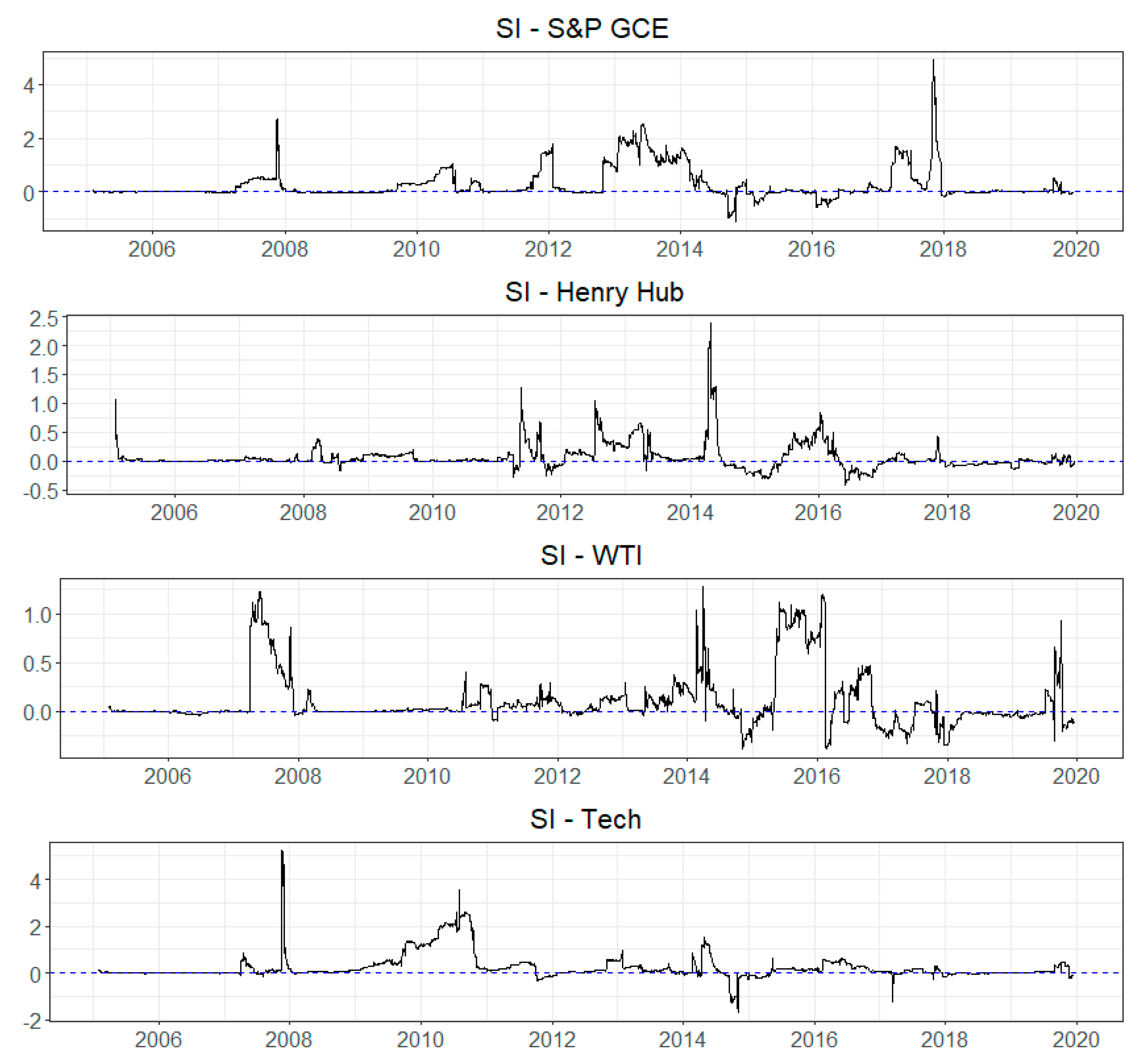
We considered the daily data of five variables in our study to analyze the connectedness measures across clean energy and other assets in the system, including clean energy stock, natural gas, crude oil, technology stock, and the investor sentiment index. The sample period was from 1 February 2005 to 20 December 2019. All variables were obtained from Bloomberg, except for the investor sentiment index. Figure 1 captures the variation in variables in the sample period.

3.1.1. Data Sources

For the clean energy index, we applied the S&P Global Clean stock index (S&P GCE) as a proxy for the performance of the global clean energy market. The S&P GCE is a weighted index comprising 30 companies around the world related to clean energy businesses. The Henry Hub natural gas and WTI crude oil are widely used as the benchmarks of the natural gas and crude oil prices, respectively. Therefore, we used the futures price of the Henry Hub and WTI to represent the fossil energy market. In addition, the NYSE Arca Tech 100 index was applied as a measurement of the technology companies’ stock performance.

3.1.2. Sentiment Analysis

The news headline sentiment regarding clean energy was used as a proxy of the investor sentiment index in this study. We applied the lexicon-based approach of sentiment analysis to construct the investor sentiment index with TextBlob tool. The TextBlob is a python library for processing textual data, which allows us to conduct sentiment analysis of a news headline in our study (the details of TextBlob are in https://textblob.readthedocs.io/en/dev/ (accessed on 28 May 2021)). The investor sentiment index was constructed in three steps. The first step was the collection of news headline data. Then, we cleaned the collected textual data (a preprocessing of data). Finally, we obtained the sentiment polarity score by a sentiment analysis by TextBlob. The specific process as follows:
First, we downloaded the news headlines dataset from Kaggle (the news headline texts were sourced from the Australian Broadcasting Corporation (ABC)), containing all the news headlines on the ABC website and focused on international news. The news dataset ranges from early 2003 to the end of 2019, collected by Rohit Kulkarni. The details on the news dataset can be found online https://www.kaggle.com/therohk/million-headlines (accessed on 1 March 2021)). To analyze whether investment sentiment affects clean energy stock, we paid attention to the news headlines related to clean energy, not all news headlines. To analyze whether investment sentiment affects clean energy stock, we paid attention to the news headlines related to clean energy, not all news headlines. Thus, we collected information by choosing news headlines with some keywords related to clean energy from the raw news dataset (the keywords related to clean energy are listed in Appendix B).
Next, we performed a preprocessing of the collected news headline textual data before the sentiment analysis. The preprocessing procedure as follows:
(a)
converting all headlines to lower case.
(b)
converting numbers into words.
(c)
expanding abbreviations.
(d)
converting symbols into words.
(e)
removing punctuations.
(f)
removing stop words.
In the lexicon-based sentiment analysis approach, we can obtain a sentiment polarity score of a word or sentence based on the sentiment lexicon. The sentiment polarity score ranged between −1 and 1, where −1, 0, and 1 represent extremely negative, neutral, and extremely positive sentiments, respectively. Our study used the TextBlob tool to calculate the sentiment polarity score of each news headline. Since there may have been many news headlines in a day, the daily sentiment polarity score as the investor sentiment index was calculated as: S I t = i = 1 n S I i t N t , where S I i t is the sentiment score of news headline i at time t, and N t is the number of news headline at time t.

3.2. Summary Statistics

The summary statistics of the variables are presented in Table 1. We calculated the logarithmic returns for S&P GCE, Henry Hub, WTI, and Tech. WE obtained the volatility of each return by fitting the AR-GARCH model. The order of AR-GARCH model was selected using the Akaike Information Criterion: AR(4)-GARCH(1,1) for S&P GCE; AR(2)-GARCH(1,1) for Henry Hub; AR(1)-GARCH(1,1) for WTI; and AR(1)-GARCH(1,1) for Tech.
From Table 1, we found that the means of WTI and Tech returns are positive, while S&P GCE and Henry Hub have negative mean returns. Table 1 shows that all the series are positively skewed except the returns of S&P GCE and Tech, and all the return and volatility series are leptokurtic. From the results of the Jarque and Bera (JB) test [28], we found that all the series returns and volatility are non-normally distributed at the 1% significance level. We must ensure all series are stationary before fitting the TVP-VAR model. Thus, using ERS unit root test [29], we found that the null hypothesis that each series has a unit root is rejected at the 1% significance level for all series. The results of the weighted Ljung-Box of Fisher and Gallagher [30] indicate that all series are significantly autocorrelated in both the series and the squared series. This implies that each series has time-varying variances; thus, employing the TVP-VAR model in this study seemed to be an appropriate econometric framework.

4. Empirical Results and Discussion

This section reports the results of the connectedness across S&P GCE, Henry Hub natural gas, WTI crude oil, technology stock (Tech), and investor sentiment (SI) from estimating the TVP-VAR-based connectedness approach proposed by Antonakakis and Gabauer [21]. The results are based on the variance decomposition of the 10 days ahead forecast horizon, and the lag order of TVP-VAR was selected by the Bayesian information criterion (BIC) (the lag is one in both the return and volatility systems).

4.1. Averaged Dynamic Connectedness Measures

Table 2 and Table 3 report the results of the average dynamic connectedness measures across the returns and volatilities of S&P GCE, Henry Hub, WTI, Tech, and SI considered in our sample using the TVP-VAR-based connectedness approach.
According to the definition of the connectedness index, we focused on the off-diagonal elements, which show the directional connectedness (e.g., the ijth entry presents the average directional connectedness from market j to market i). The From column exhibits the average total connectedness received by one asset from all the other assets, while the to row reports the average total connectedness transmits from one asset to all other assets in the full sample. Net is the average net total connectedness of market i, which determines the net transmitter (contributor) or net receiver of the connectedness in the system (To-From). Total represents the average of the total dynamic connectedness in the system.
Table 2 displays the estimated return spillover indices across five variables, which helps us to understand the direction and average strength of dynamic return connectedness across S&P GCE, Henry Hub, WTI, Tech, and SI over the full sample period. The results in Table 2 show that the total return connectedness was 20.4%, indicating the 20.4% total forecast error variance in the system was from crossvariables. This reveals that there was an interrelation among the asset returns in the system.
In the To row, S&P GCE contributes most to the GFEVD of the other variables in the system (37.0%), followed by Tech (34.6%), WTI (19.7%), Henry Hub (8.2%), and SI (2.5%). For the From column, S&P GCE receives 35.5% from the other variables, followed by Tech (33.0%), WTI (21.0%), Henry Hub (9.5%), and SI (3%). Thus, S&P GCE was the largest contributor and receiver of total return spillover, while the investor sentiment index transmitted and received the least return spillover in the system. With regard to Net, we found that S&P GCE and Tech were the net (total) contributors and other assets were the net (total) receivers of return spillover in this system.
Following the pairwise connectedness results of S&P GCE in the first row in Table 2, we identified that Tech was the largest contributor of the S&P GCE return spillover and SI transmits the least return spillover to S&P GCE, which implies that the technology stock had a more significant impact on the clean energy stock return in this system. Moreover, the results also indicated that the impact of investor sentiment on the clean energy stock was less than that of other assets in the system. This finding is consistent with previous literature, in which Song et al. [15] obtained the same result, that investor sentiment has a small impact on the renewable energy stock, by analyzing the relationship between investor sentiment and renewable energy stock.
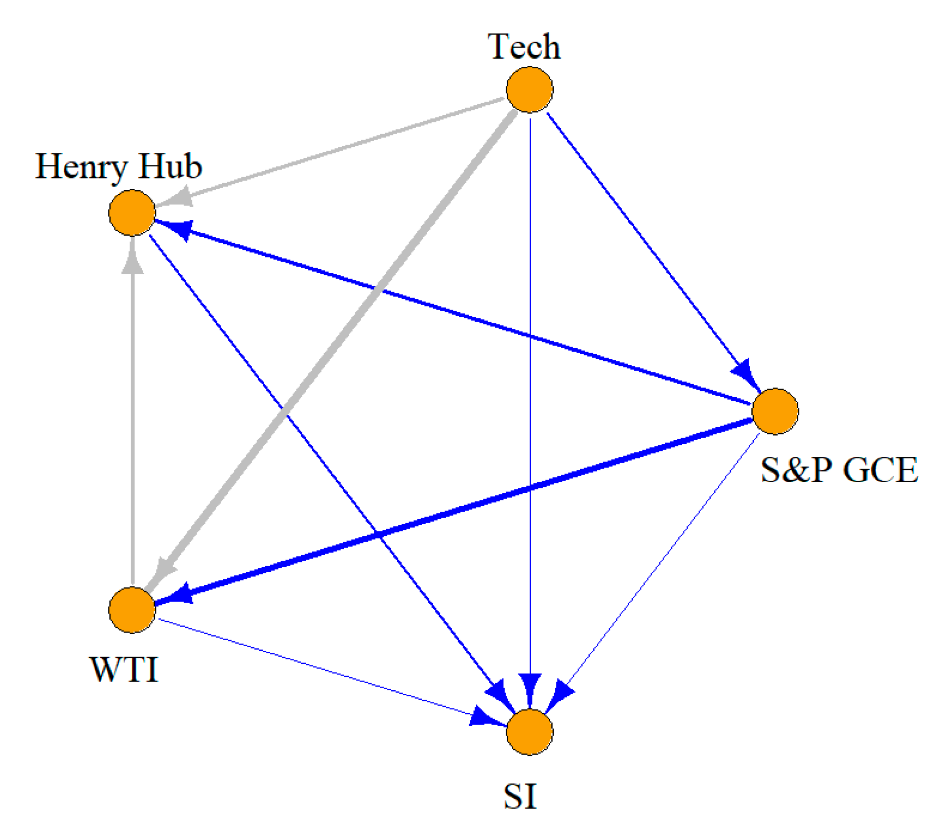
Figure 2 displays the net pairwise directional connectedness network across each variable, which allows us to identify the direction and intensity of the net return connectedness from one variable to another variable in the system. The nodes represent the variables in the system, whereas the direction of the arrows indicates the transmission direction of the net pairwise connectedness between a pair of variables. The thickness of the edges represents the strength of the net pairwise connectedness across variables. We use blue edges of S&P GCE and SI nodes to highlight the performance of S&P GCE and SI in the network system.
In Figure 2, the direction of arrows is from S&P GCE to WTI, Henry Hub, and SI, suggesting that S&P GCE contributed more return spillover to WTI, Henry Hub, and SI than received spillover from them. Tech contributed more return spillover to S&P GCE than S&P GCE contributed to it. It was worth noting that SI was a net pairwise connectedness receiver of other variables in the return system, which suggested that other variables significantly impact SI in the full sample. As mentioned earlier, the thickness of the edges is the strength of net pairwise connectedness; the thicker the edge, the greater the difference between the two variables’ pairwise directional spillover. We concluded that the net pairwise directional connectedness between S&P GCE and WTI was highest from the finding of the thickest edge in the network being between S&P GCE and WTI.
The volatility connectedness indices across five variables in the full sample are presented in Table 3. The total volatility connectedness was 23.8%, which is higher than the total return connectedness (20.4%), suggesting a higher level of information transmission across the assets in the volatility system.
Per the From and To in Table 3, Tech received the most volatility spillover (41.5%) from the other variables, while S&P GCE was the most significant contributor (39.8%) of the volatility spillover in this system. In terms of the net (total) connectedness index, S&P GCE and SI were the net volatility contributors; and Henry Hub, WTI, and Tech were the net receivers of volatility connectedness, which is slightly different from the return connectedness result.
As shown by the pairwise connectedness results of S&P GCE in Table 3, Tech still transmitted the most spillover to the S&P GCE volatility, whereas SI contributed the least volatility spillover to S&P GCE.
Overall, both in the return and volatility systems, S&P GCE received more spillover from Tech than from Henry Hub and WTI, which implies that the relationship between clean energy stock and technology stock was closer than the relationship between clean energy stock and fossil fuel commodities. Our results are consistent with previous literature [4,7,31]. For example, Sadorsky [7] analyzed the relationship between clean energy companies’ stock prices, technology companies’ stock prices, and oil prices. The results showed that the clean energy companies’ stock prices more strongly correlated with technology stock prices than oil prices. According to our findings, the investors interested in clean energy stock should consider fossil fuel commodities in their portfolio to increase their diversification benefits.
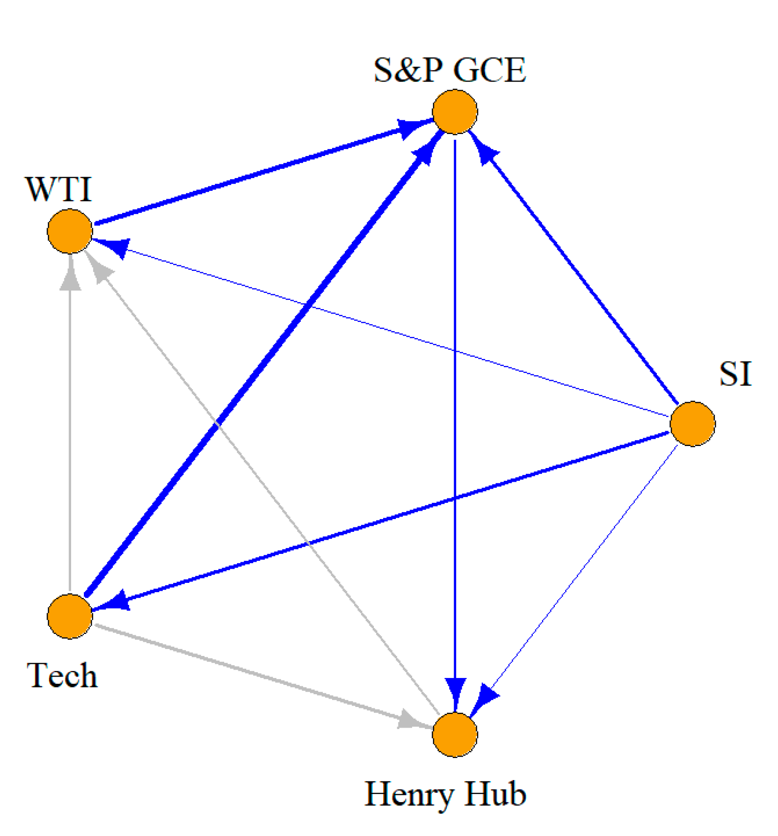
The net pairwise directional volatility connectedness network is shown in Figure 3. Around the S&P GCE node, the direction of arrows is from Tech, WTI, and SI to S&P GCE. This suggests that Tech, WTI, and SI had a more critical impact on S&P GCE than they were affected by it over the sample period. The direction of the arrow being from S&P GCE to Henry Hub means that S&P GCE contributed more volatility spillover to Henry Hub than it received spillover from it. The highest net pairwise directional connectedness was between S&P GCE and Tech. Interestingly, contrary to the return system result, SI was a net pairwise connectedness transmitter of other variables in the volatility system. It suggested that SI is a valuable tool to predict the performance of the S&P GCE volatility and other variable volatility.

4.2. Dynamic Connectedness Measures

The full-sample results presented in Table 2 and Table 3 only consider the average dynamic spillover indices over the whole sample period and ignore the variation in the spillover indices over time in the sample. Therefore, we focused on the dynamic connectedness across S&P GCE, Henry Hub natural gas, WTI crude oil, technology stock, and investor sentiment over time.

4.2.1. Dynamic Total Connectedness Analysis

The dynamic total return connectedness is plotted in Figure 4. The dynamic total return connectedness index ranged between 12% and 35% and changed considerably over time, which implies that the degree of information transmission across assets in this system varied with time. From Figure 4, several significant spikes can be observed during the periods of 2008–2009, 2011–2012, and 2018–2019, with an approximately 20% uplift in the total connectedness during those periods. Those could be attributed to emergency events, such as the global financial crisis in 2008, the European sovereign debt crisis in 2011, and the China–United States trade war in 2018. In line with previous literature [32,33,34], our study provides evidence that supports the notion that the connectedness across different assets increases rapidly during financial turmoil. The dynamic connectedness exhibited some significant decreases (e.g., 2012–2014) after the turmoil in the financial market; a reasonable explanation for those decreases could be the economic recovery and economic prosperity.
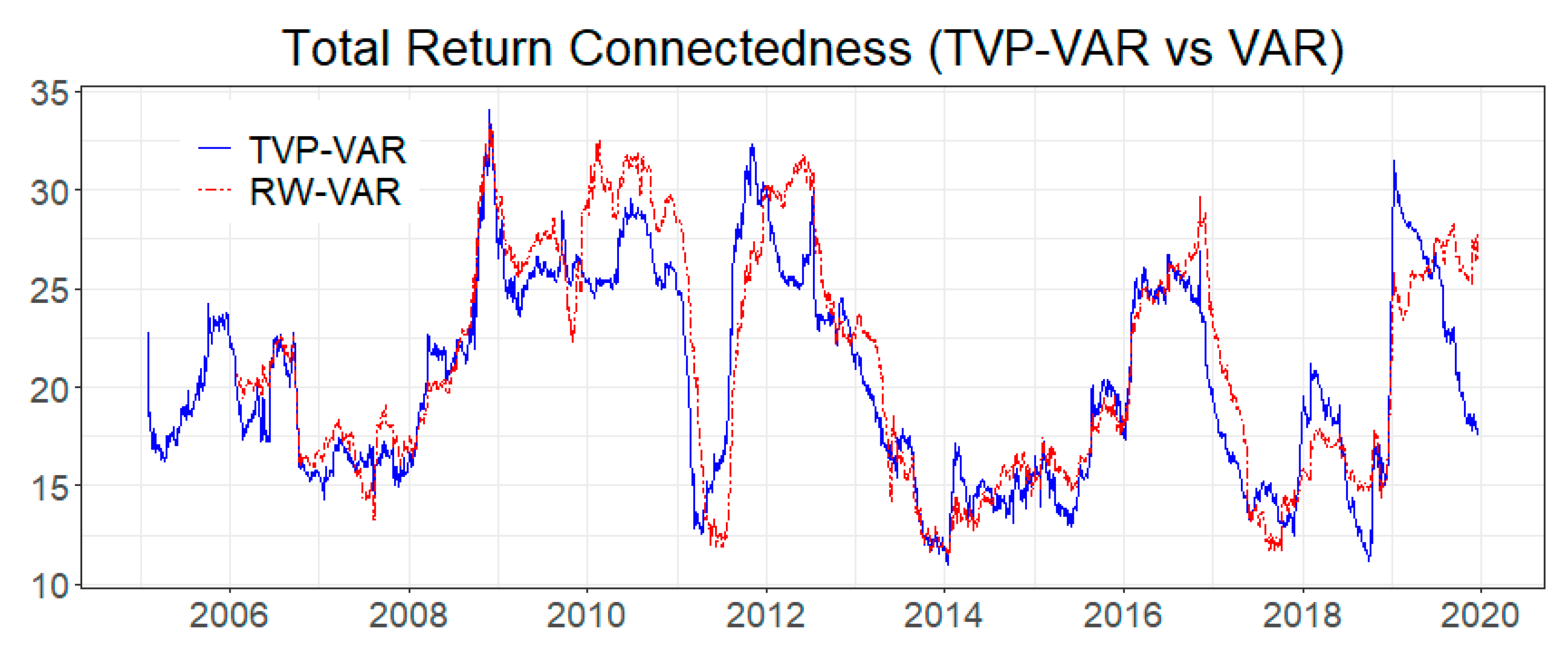
To compare the dynamic connectedness indices estimated by traditional VAR, we applied a 200 day rolling window to capture the variation in total connectedness estimated by the VAR-based Diebold–Yilmaz approach over time. Figure 5 shows the comparison results. The blue line (solid line) resulted from the TVP-VAR-based connectedness measures, and the red line (two-dash line) was the rolling-window VAR-based connectedness measures results. We observed that the observations of rolling-window VAR-based connectedness measures are less than those of TVP-VAR-based connectedness measures. This finding confirmed that the rolling-window VAR-based connectedness measures would lose some observations in the sample. It further reflected that one of the advantages of TVP-VAR-based connectedness measures was that it would not lose any observations.
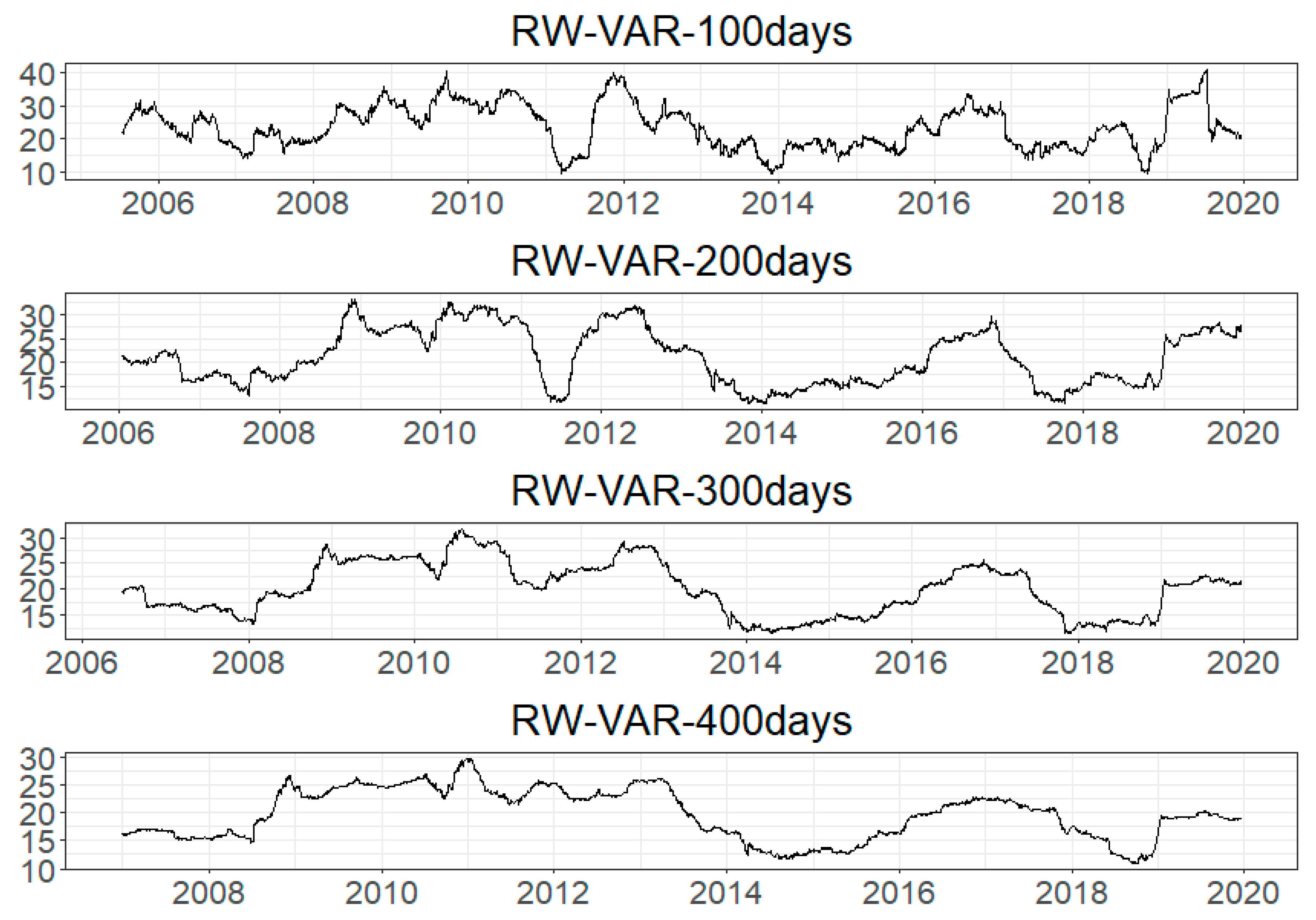
Interestingly, the trend in dynamic total return connectedness based on the TVP-VAR is similar to the dynamic total return connectedness based on the traditional VAR-based Diebold–Yilmaz approach. Furthermore, the traditional dynamic total return connectedness shows the same sharp fluctuations during the financial turmoil. We also found that the strength of the dynamic connectedness indices estimated by the traditional VAR changes with a rolling-window size; the trend in connectedness indices becomes flat with a larger window length (we present the comparison of dynamic total spillover with different window lengths in Figure A1 in Appendix B). In other words, the VAR-based connectedness measures with a rolling window may ignore some variation in connectedness in the sample, which may affect investment decisions.
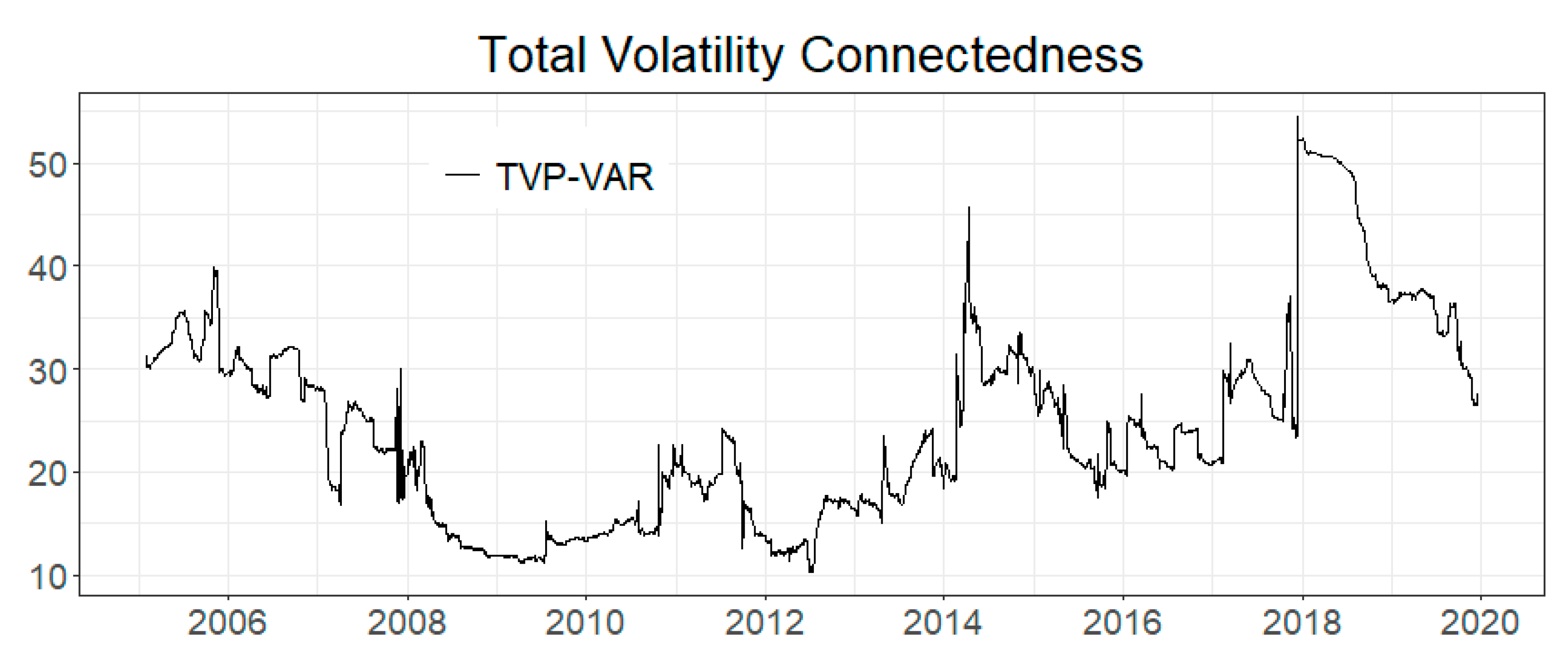
Figure 6 shows the dynamic total spillover across asset volatilities. The variation in volatility connectedness ranged between 10% and 55% in the sample, which is more dramatic in comparison with the total return connectedness in Figure 4. Interestingly, total volatility connectedness significantly increased in 2014, but this rise was not obvious in total return connectedness. This rise could be related to the crude oil crisis in 2014. It implied the volatility connectedness has a more intense reaction than return connectedness to this crude oil crisis. Moreover, the degree of changes in dynamic total volatility connectedness in financial turmoil is higher than in total return connectedness. These findings suggest that volatility connectedness is more sensitive than return connectedness, especially during financial turmoil. The findings also revealed that the correlations across S&P GCE, Henry Hub, WTI, Tech, and SI volatilities were closer than those of returns during financial turmoil. The information transmission of the volatility system is more effective than the return system when financial events occur.
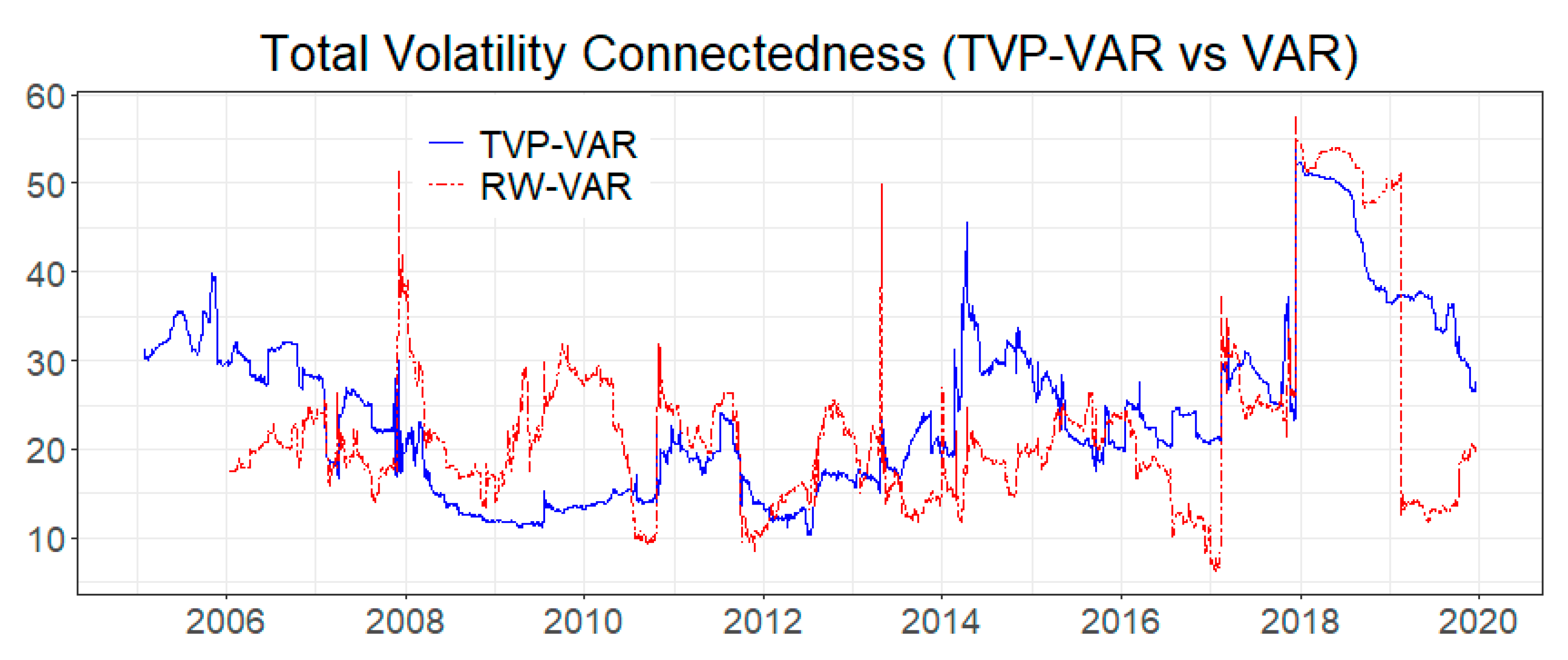
In Figure 7, we compare the volatility connectedness calculated by the dynamic connectedness measures based on the TVP-VAR with that of the 200 day rolling-window VAR model. Though the volatility connectedness estimated based on the VAR model showed a different trend in the sample, the volatility connectedness based on the rolling-window VAR model also increased significantly during financial turmoil, which is similar to the results of the volatility connectedness based on the TVP-VAR model.

4.2.2. Dynamic Net Connectedness Analysis

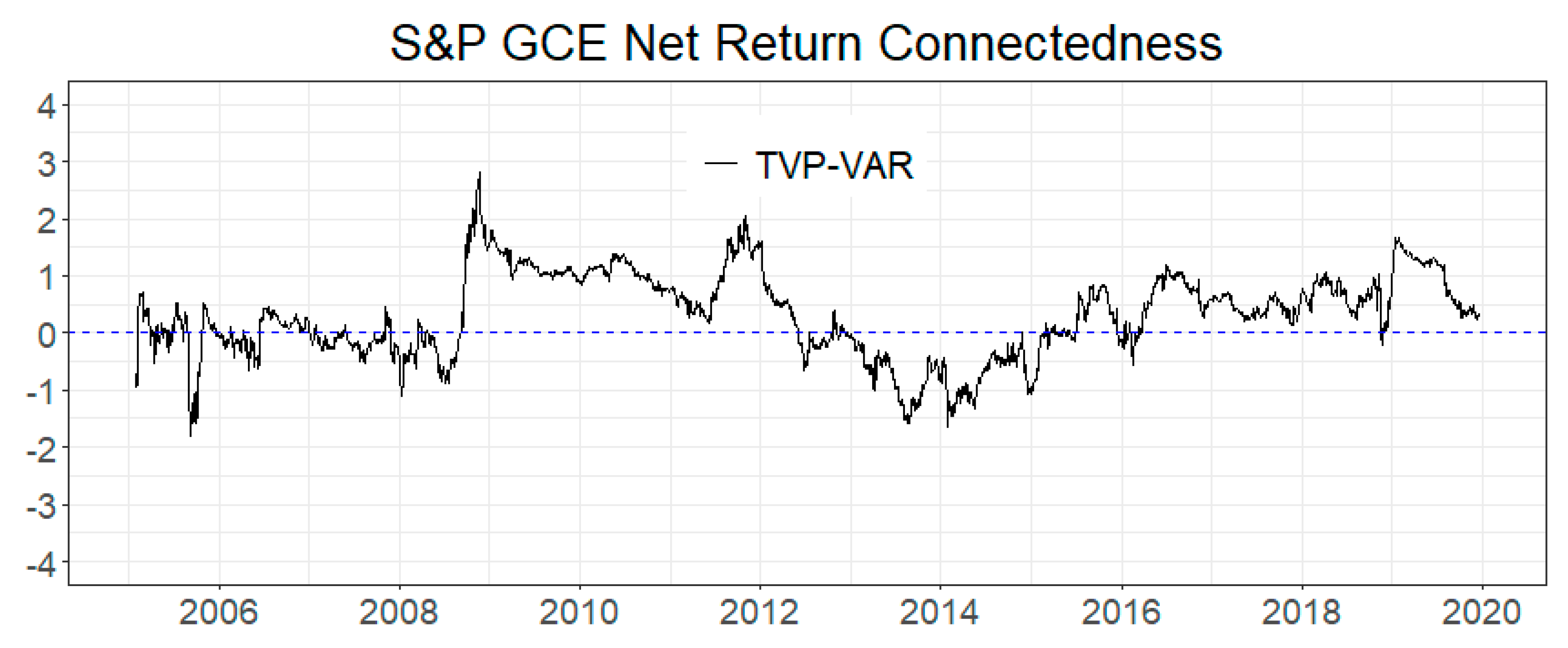
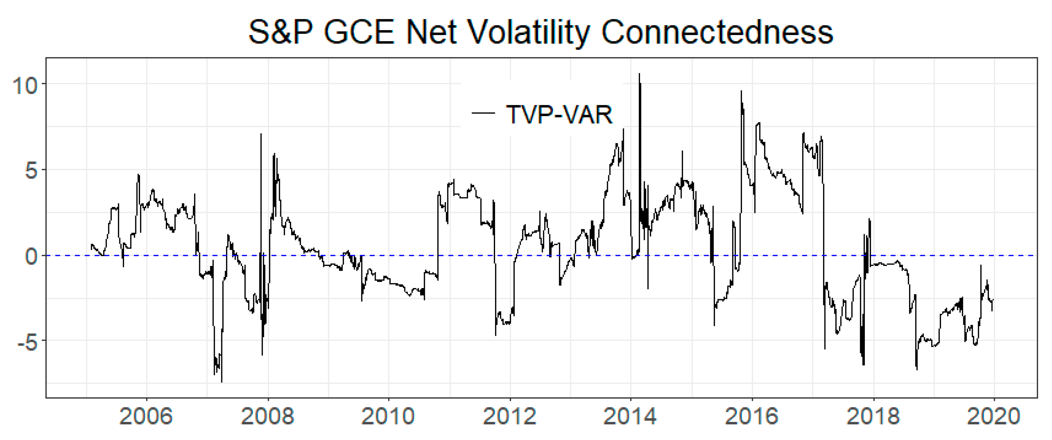
Since we focused more on clean energy investment, Figure 8 and Figure 9 outline the dynamic net return and volatility connectedness of S&P GCE. The net connectedness changing between positive and negative values in the sample reveals that S&P GCE was not a simple receiver in this system and further reflected the importance of the dynamic analysis of connectedness. During the GFC period, S&P GCE transformed from a net receiver to a contributor in the return system, while S&P GCE was a contributor in the European sovereign debt crisis and China–United States trade war.
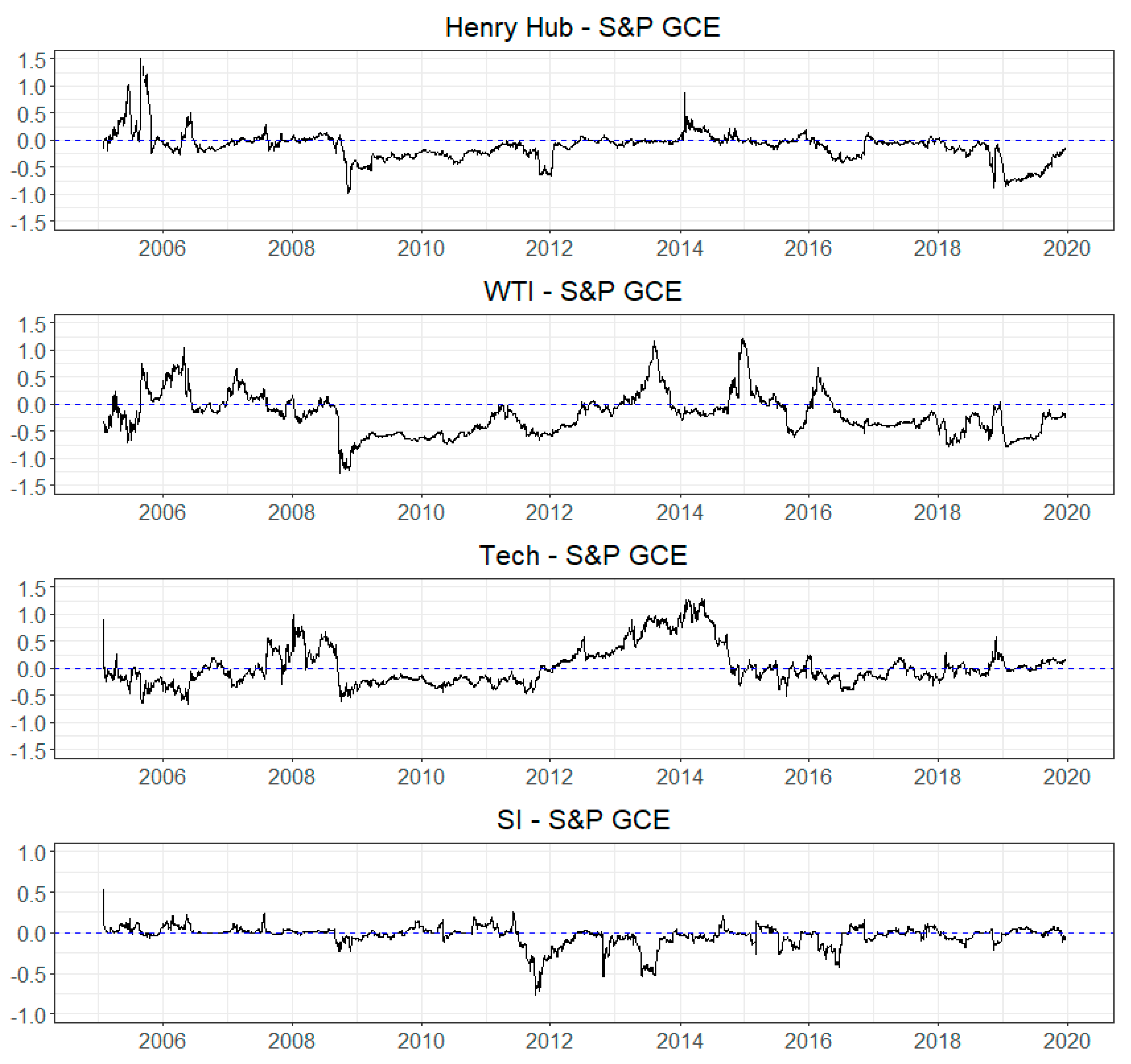
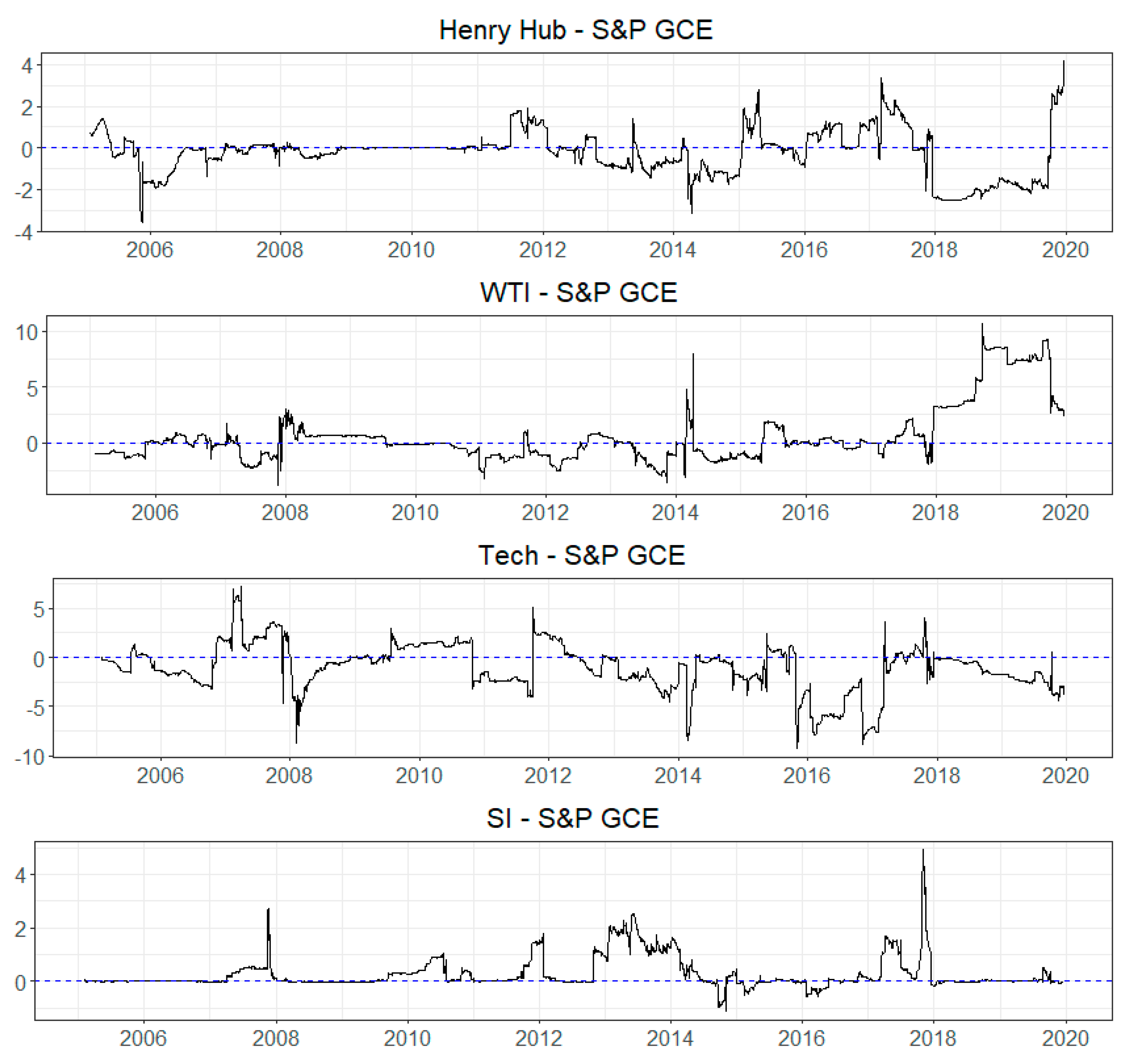
We also capture the net pairwise spillover between S&P GCE and the other variables in Figure A2 and Figure A3 in Appendix B. The results shown in Figure A2 and Figure A3 indicate that the net pairwise connectedness between S&P GCE and other assets changed drastically during financial turmoil. The findings provide useful information for investors. An investor may diversify the assets by considering the net pairwise spillover between S&P GCE and the other assets. Since the net pairwise spillover varies with time, investors should adjust their portfolios in time, especially when financial events occur.
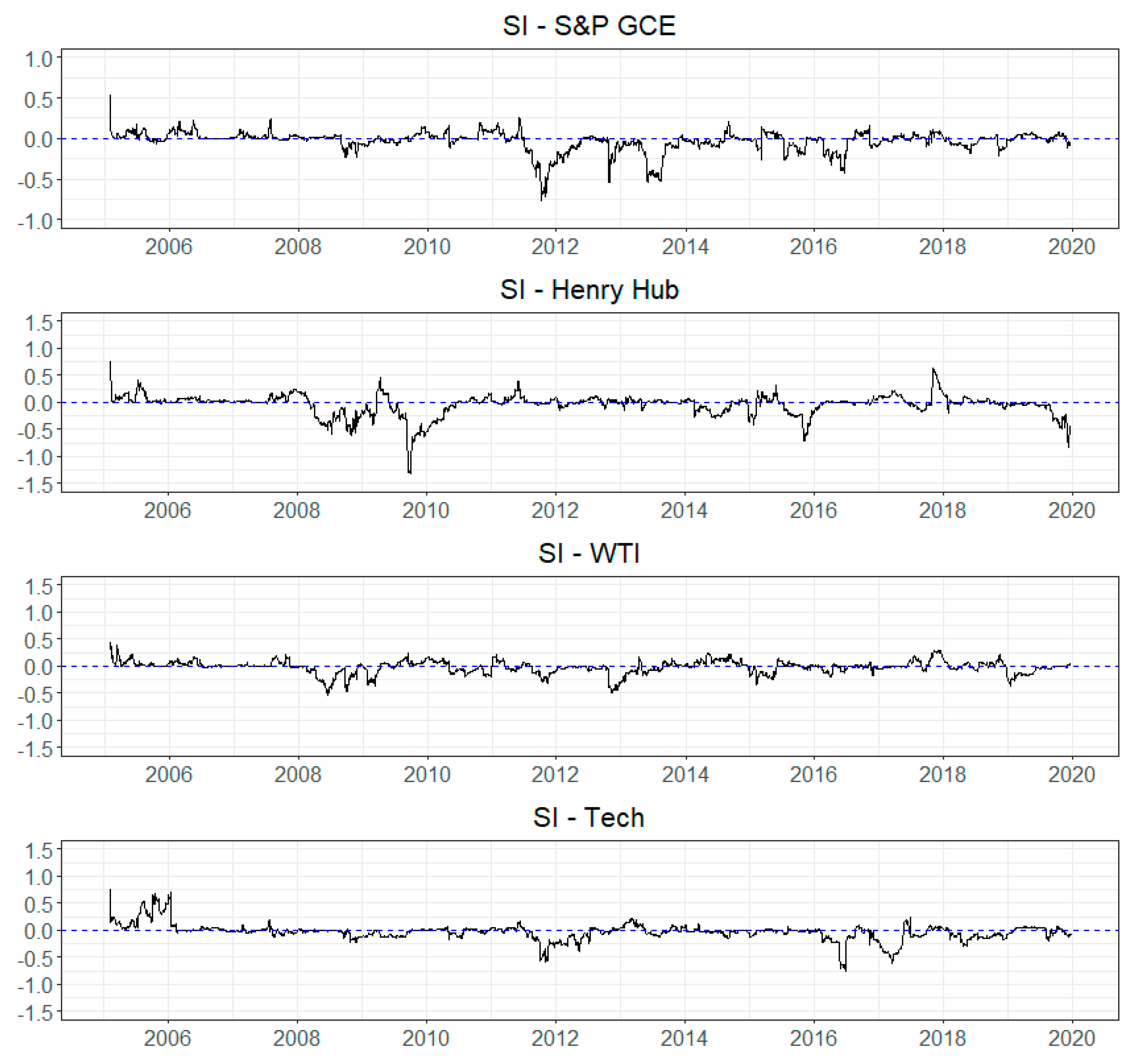
The dynamic net pairwise return and volatility spillover between SI and the other variables are presented in Figure A4 and Figure A5 in Appendix B. In Figure A5, we found that in most economic events, SI was a net pairwise transmitter in the pair of SI and the other variables. This finding implies that the impact of SI on S&P GCE, Tech, and fossil fuel volatility strengthened significantly in most economic events. From this result, we may speculate that investor sentiment significantly affects the stock market and commodities volatility in economic events.

5. Conclusions

In this study, we investigated the interaction across the return and volatility of clean energy stock, technology stock, fossil energy, and investor sentiment from 2005 to 2019. Specifically, we constructed a system comprising S&P GCE clean energy stock, NYSE Arca technology stock, WTI crude oil, Henry Hub natural gas, and investor sentiment, using a TVP-VAR-based dynamic connectedness approach. To the best of our knowledge, no study has previously covered this field in the literature, and our study fills this gap. Moreover, we compared the dynamic total connectedness estimated by the TVP-VAR-based connectedness approach and that was estimated by the rolling-window VAR-based connectedness approach.
The main empirical results are as follows: First, the average total dynamic connectedness was higher in the volatility system than in the return system. Second, both in the return and volatility systems, the technology stock contributed the most spillover, while investor sentiment transmitted the least spillover, to the clean energy stock. Third, the dynamic total connectedness across assets in terms of return and volatility varied with time and showed a noticeable increase during financial turmoil. We also found that the dynamic total volatility connectedness changed more dramatically and rapidly during abrupt events. Fourth, the dynamic total return connectedness of the TVP-VAR model is similar to the estimated results of a 200 day rolling-window VAR model.
The innovation of this study as follows: First, to the best of our knowledge, this is the first study to examine the interaction of the return and volatility of S&P GCE clean energy stock, NYSE Arca technology stock, WTI crude oil, Henry Hub natural gas, and investor sentiment. Second, we employed an investor sentiment index by collecting the information from clean-energy-related news headlines. The main differences in this index compared to other indexes used for analyzing investor sentiment and clean energy are the information sources and lengths. The length of our investor sentiment series is over a decade. Thus, one advantage of this investor sentiment index is that it covers enough information so that variations in the sample caused by some financial crises in past times are not lost due to too short a time period. Third, we used a TVP-VAR-based connectedness approach to calculate the dynamic connectedness across assets in the return and volatility systems. The approach allowed us to quantify the intensity and direction of dynamic connectedness across different assets in the system. The approach does not lose observations or variation in the sample period compared with the rolling-window VAR-based connectedness approach.
Our study findings have some implications for policymakers and investors in the clean energy market. It is crucial for policymakers to strengthen the stability of the clean energy markets against exposure to risks, especially during financial turmoil. According to our evidence of the close interaction between clean energy stock and technology stock, they should pay close attention to technology company stock behavior and related policies to consider the adjustment of policies or actions in time to promote the development of clean energy. Since the connectedness across assets is dynamic and rises rapidly during financial turmoil, investors may adjust their investment portfolios and strategies in a timely manner to mitigate or circumvent losses. The investor sentiment had the weakest average impact on the clean energy stock over the full sample period. However, the impact of investor sentiment on clean energy stock and other variables volatilities increase greatly in most economic events in the sample period. Therefore, policymakers and investors should focus on investor sentiment in economic events because investor sentiment causes great fluctuations in clean energy stock volatility. In addition, the directional connectedness between natural gas and clean energy stock is the lowest; thus, considering natural gas in the clean energy portfolio may relatively reduce risk and improve the performance of the portfolio.
Some previous literature [35,36,37] had emphasized the importance of asymmetric conditional correlation in financial markets. Therefore, it would be interesting to compare the conditional correlation with dynamic pairwise connectedness in our future analysis.

Author Contributions

Investigation, T.L.; writing—original draft preparation, T.L.; writing—review and editing, S.H.; project administration, S.H.; funding acquisition, S.H. All authors have read and agreed to the published version of the manuscript.

Funding

This work was supported by JSPS KAKENHI Grant Number 17H00983.

Institutional Review Board Statement

Not applicable.

Informed Consent Statement

Not applicable.

Data Availability Statement

Not applicable.

Acknowledgments

We thank Rohit Kulkarni for allowing us to use the news dataset. We are grateful to three anonymous referees for their many helpful comments and suggestions.

Conflicts of Interest

The authors declare no conflict of interest.

Appendix A

The TVP-VAR is defined as:
y t = Φ t z t 1 + ε t           ε t | Ω t 1 ~ N ( 0 , Σ t )
v e c ( Φ t ) = v e c ( Φ t 1 ) + ξ t       ξ t | Ω t 1 ~ N ( 0 , Ξ t )
where Ω t 1 contains all the information available until t 1 . y t and z t 1 represent an N × 1 and N p × 1 dimensional vector of the observed variables, respectively. Φ t is an N × N p time-varying matrix of coefficient ε t and an N × 1 dimensional vector, and Σ t is an N × N time-varying variance matrix. Additionally, v e c ( Φ t ) and ξ t are an N 2 p × 1 dimensional vector, and Ξ t is an N 2 p × N 2 p time-varying variance matrix.
This study employs the noninformative prior, and the prior parameters Φ 0 and Σ 0 are set as follows:
v e c ( Φ 0 ) ~ N ( v e c ( 0 ,   N p · I ) Σ 0 = C o v ( y )
The Kalman filter estimation controls how fast the estimated coefficients vary over time via the forgetting factors (0 ≤ κi ≤ 1). Following Chatziantoniou and Gabauer [38], we also set the forgetting factor κ 1 = κ 2 = 0.99 .
Hence, the multivariate Kalman filter can be formulated as follows:
v e c ( Φ t ) | z 1 : t 1 ~ N ( v e c , Φ t | t 1 , Σ t | t 1 Φ ) Φ t | t 1 = Φ t 1 | t 1 ε t = y t Φ t | t 1 z t 1 Σ t = κ 2 Σ t 1 | t 1 + ( 1 κ 2 ) ε t ε t Ξ t = ( 1 κ 1 1 ) Σ t 1 | t 1 Φ Σ t | t 1 Φ = Σ t 1 | t 1 Φ + Ξ t Σ t | t 1 = z t 1 Σ t | t 1 Φ z t 1 + Σ t
We update Φ t   , Σ t Φ , and Σ t   , given the information at time t as follows:
v e c ( Φ t ) | z 1 : t ~ N ( v e c , Φ t | t , Σ t | t Φ ) Κ t = Σ t | t 1 Φ z t 1 Σ t | t 1 1 Φ t | t = Φ t | t 1 + K t ( y t Φ t | t 1 z t 1 ) Σ t | t Φ = ( Ι Κ t )   Σ t | t 1 Φ ε t | t = y t Φ t | t z t 1 Σ t | t = κ 2 Σ t 1 | t 1 + ( 1 κ 2 ) ε t | t ε t | t
where Kt represents the Kalman gain that explains by how much the parameters Φ t should be changed in the given state.

Appendix B

Table A1. Keywords used to collect news headlines related to clean energy.
biodieselphotovoltaic systemsolar resource
bioenergy photovoltaicssolar techniques
biofuel pollution free energysolar thermal
biomasspower generationsolar thermal collector
carbon neutral renewablesolar thermal energy
clean energyrenewable energysolar thermal power systems
climaterenewable heatsolar tower
climate change renewable thermal energysolar towers
concentrated solar powerrenewables power capacitysolar tracker
energysolarsolar water heater
environmentsolar air sustainable
environmentalsolar air conditioningtidal
genesis solar energy projectsolar air heattidal energy
geothermalsolar air heatingtidal power
geothermal developmentsolar cellvariable renewable energy
geothermal energysolar cell efficiencywater power
geothermal heat pumpssolar cellswatermill
geothermal power plantssolar collectorwatermills
global warmingsolar combisystemwave
greensolar cookerwave energy
green energysolar desalinationwave energy converter
green wastesolar energywave farm projects
ground source heat pumpsolar energy generating systemswave hub
hydroelectricsolar energy projectwave power
hydroelectric powersolar fuelwaves and tides
hydroelectric power plants solar furnacewind
hydroelectricitysolar generating stationwind energy
hydropowersolar heatwind farm
hydropower resourcesolar heatingwind farms
marine and hydrokinetic energysolar hot waterwind park
marine energy solar hot water capacitywind parks
marine powersolar hot water heatingwind power
molten salt heat storagesolar irradiancewind power plant
ocean energysolar moduleswind power station
ocean powersolar panelwind project
ocean power technologiessolar powerwind projects
ocean thermal energy conversionsolar power stationwind turbine
ocean wavessolar power towerwind turbines
parabolic troughsolar pv capacitywind waves
photovoltaic developmentsolar pv
Figure A1. Dynamic total return connectedness via VAR-based connectedness approach with 100, 200, 300, and 400 days.
Energies 14 03442 g0a1
Figure A2. Dynamic net pairwise directional return connectedness (S&P GCE). Note: S&P GCE indicates Standard & Poor Global Clean Energy Index; Henry Hub indicates Henry Hub Natural Gas Futures; WTI indicates West Texas Intermediate Crude Oil Futures; Tech indicates NYSE Arca Tech 100 Index; SI indicates investor sentiment index.
Energies 14 03442 g0a2
Figure A3. Dynamic net pairwise directional volatility connectedness (S&P GCE).
Energies 14 03442 g0a3
Figure A4. Dynamic net pairwise directional return connectedness (SI).
Energies 14 03442 g0a4
Figure A5. Dynamic net pairwise directional volatility connectedness (SI).
Energies 14 03442 g0a5

References

  1. Liu, T.; Hamori, S. Spillovers to Renewable Energy Stocks in the US and Europe: Are They Different? Energies 2020, 13, 3162. [Google Scholar] [CrossRef]
  2. Xia, T.; Ji, Q.; Zhang, D.; Han, J. Asymmetric and extreme influence of energy price changes on renewable energy stock performance. J. Clean. Prod. 2019, 241, 118338. [Google Scholar] [CrossRef]
  3. Uddin, G.S.; Rahman, M.L.; Hedström, A.; Ahmed, A. Cross-quantilogram-based correlation and dependence between renewable energy stock and other asset classes. Energy Econ. 2019, 80, 743–759. [Google Scholar] [CrossRef]
  4. Reboredo, J.C.; Ugolini, A. The impact of energy prices on clean energy stock prices. A multivariate quantile dependence approach. Energy Econ. 2018, 76, 136–152. [Google Scholar] [CrossRef]
  5. Henriques, I.; Sadorsky, P. Oil prices and the stock prices of alternative energy companies. Energy Econ. 2008, 30, 998–1010. [Google Scholar] [CrossRef]
  6. Ahmad, W. On the dynamic dependence and investment performance of crude oil and clean energy stocks. Res. Int. Bus. Financ. 2017, 42, 376–389. [Google Scholar] [CrossRef]
  7. Sadorsky, P. Correlations and volatility spillovers between oil prices and the stock prices of clean energy and technology companies. Energy Econ. 2012, 34, 248–255. [Google Scholar] [CrossRef]
  8. Kumar, S.; Managi, S.; Matsuda, A. Stock prices of clean energy firms, oil and carbon markets: A vector autoregressive analysis. Energy Econ. 2012, 34, 215–226. [Google Scholar] [CrossRef]
  9. Bahloul, W.; Bouri, A. The impact of investor sentiment on returns and conditional volatility in US futures markets. J. Multinatl. Financ. Manag. 2016, 36, 89–102. [Google Scholar] [CrossRef]
  10. Yang, C.; Gao, B. The term structure of sentiment effect in stock index futures market. N. Am. J. Econ. Financ. 2014, 30, 171–182. [Google Scholar] [CrossRef]
  11. Aloui, C.; Hkiri, B.; Lau, C.K.M.; Yarovaya, L. Investors’ sentiment and US Islamic and conventional indexes nexus: A time-frequency analysis. Financ. Res. Lett. 2016, 19, 54–59. [Google Scholar] [CrossRef]
  12. Ji, Q.; Li, J.; Sun, X. Measuring the interdependence between investor sentiment and crude oil returns: New evidence from the CFTC’s disaggregated reports. Financ. Res. Lett. 2019, 30, 420–425. [Google Scholar] [CrossRef]
  13. Dergiades, T. Do investors’ sentiment dynamics affect stock returns? Evidence from the US economy. Econ. Lett. 2012, 116, 404–407. [Google Scholar] [CrossRef] [Green Version]
  14. Reboredo, J.C.; Ugolini, A. The impact of twitter sentiment on renewable energy stocks. Energy Econ. 2018, 76, 153–169. [Google Scholar] [CrossRef]
  15. Song, Y.; Ji, Q.; Du, Y.J.; Geng, J.B. The dynamic dependence of fossil energy, investor sentiment and renewable energy stock markets. Energy Econ. 2019, 84, 104564. [Google Scholar] [CrossRef]
  16. Liu, T.; He, X.; Nakajima, T.; Hamori, S. Influence of Fluctuations in Fossil Fuel Commodities on Electricity Markets: Evidence from Spot and Futures Markets in Europe. Energies 2020, 13, 1900. [Google Scholar] [CrossRef] [Green Version]
  17. Zhang, Y.; He, X.; Nakajima, T.; Hamori, S. Oil, Gas, or Financial Conditions-Which One Has a Stronger Link with Growth? N. Am. J. Econ. Financ. 2020, 54, 101220. [Google Scholar] [CrossRef]
  18. Zhang, W.; Hamori, S. Crude oil market and stock markets during the COVID-19 pandemic: Evidence from the US, Japan, and Germany. Int. Rev. Financ. Anal. 2021, 74, 101702. [Google Scholar] [CrossRef]
  19. Diebold, F.X.; Yilmaz, K. On the network topology of variance decompositions: Measuring the connectedness of financial firms. J. Econom. 2014, 182, 119–134. [Google Scholar] [CrossRef] [Green Version]
  20. Antonakakis, N.; Gabauer, D. Refined Measures of Dynamic Connectedness Based on TVP-VAR. Available online: https://mpra.ub.uni-muenchen.de/id/eprint/78282 (accessed on 1 April 2021).
  21. Bouri, E.; Cepni, O.; Gabauer, D.; Gupta, R. Return connectedness across asset classes around the COVID-19 outbreak. Int. Rev. Financ. Anal. 2021, 73, 101646. [Google Scholar] [CrossRef]
  22. Antonakakis, N.; Gabauer, D.; Gupta, R.; Plakandaras, V. Dynamic connectedness of uncertainty across developed economies: A time-varying approach. Econ. Lett. 2018, 166, 63–75. [Google Scholar] [CrossRef] [Green Version]
  23. Gabauer, D.; Gupta, R. On the transmission mechanism of country-specific and international economic uncertainty spillovers: Evidence from a TVP-VAR connectedness decomposition approach. Econ. Lett. 2018, 171, 63–71. [Google Scholar] [CrossRef] [Green Version]
  24. Koop, G.; Korobilis, D. A new index of financial conditions. Eur. Econ. Rev. 2014, 71, 101–116. [Google Scholar] [CrossRef] [Green Version]
  25. Antonakakis, N.; Chatziantoniou, I.; Gabauer, D. Refined measures of dynamic connectedness based on time-varying parameter vector autoregressions. J. Risk Financ. Manag. 2020, 13, 84. [Google Scholar] [CrossRef]
  26. Koop, G.; Pesaran, M.H.; Potter, S.M. Impulse response analysis in non-linear multivariate models. J. Econom. 1996, 74, 119–147. [Google Scholar] [CrossRef]
  27. Pesaran, H.H.; Shin, Y. Generalized impulse response analysis in linear multivariate models. Econ. Lett. 1998, 58, 17–29. [Google Scholar] [CrossRef]
  28. Jarque, C.M.; Bera, A.K. Efficient tests for normality homoscedasticity and serial independence of regression residuals. Econ. Lett. 1980, 6, 255–259. [Google Scholar] [CrossRef]
  29. Elliott, G.; Rothenberg, T.J.; Stock, J.H. Efficient Tests for an Autoregressive Unit Root; Technical Working Paper 0130; National Bureau of Economic Research: Cambridge, MA, USA, 1992. [Google Scholar] [CrossRef]
  30. Fisher, T.J.; Gallagher, C.M. New weighted portmanteau statistics for time series goodness of fit testing. J. Am. Stat. Assoc. 2012, 107, 777–787. [Google Scholar] [CrossRef]
  31. Manage, S.; Okimoto, T. Does the price of oil interact with clean energy prices in the stock market? Jpn. World Econ. 2013, 27, 1–9. [Google Scholar] [CrossRef] [Green Version]
  32. Li, L.; Yin, L.; Zhou, Y. Exogenous shocks and the spillover effects between uncertainty and oil price. Energy Econ. 2016, 54, 224–234. [Google Scholar] [CrossRef]
  33. Křehlík, T.; Baruník, J. Cyclical properties of supply-side and demand-side shocks in oil-based commodity markets. Energy Econ. 2017, 65, 208–218. [Google Scholar] [CrossRef] [Green Version]
  34. Ferrer, R.; Shahzad, S.J.H.; López, R.; Jareño, F. Time and frequency dynamics of connectedness between renewable energy stocks and crude oil prices. Energy Econ. 2018, 76, 1–20. [Google Scholar] [CrossRef]
  35. Ang, A.; Chen, J. Asymmetric correlations of equity portfolios. J. Financ. Econ. 2002, 63, 443–494. [Google Scholar] [CrossRef]
  36. Hong, Y.; Tu, J.; Zhou, G. Asymmetries in stock returns: Statistical tests and economic evaluation. Rev. Financ. Stud. 2007, 20, 1547–1581. [Google Scholar] [CrossRef]
  37. Longin, F.; Solnik, B. Extreme correlation of international equity markets. J. Financ. 2001, 56, 649–676. [Google Scholar] [CrossRef]
  38. Chatziantoniou, I.; Gabauer, D. EMU risk-synchronisation and financial fragility through the prism of dynamic connectedness. Q. Rev. Econ. Financ. 2021, 79, 1–14. [Google Scholar] [CrossRef]
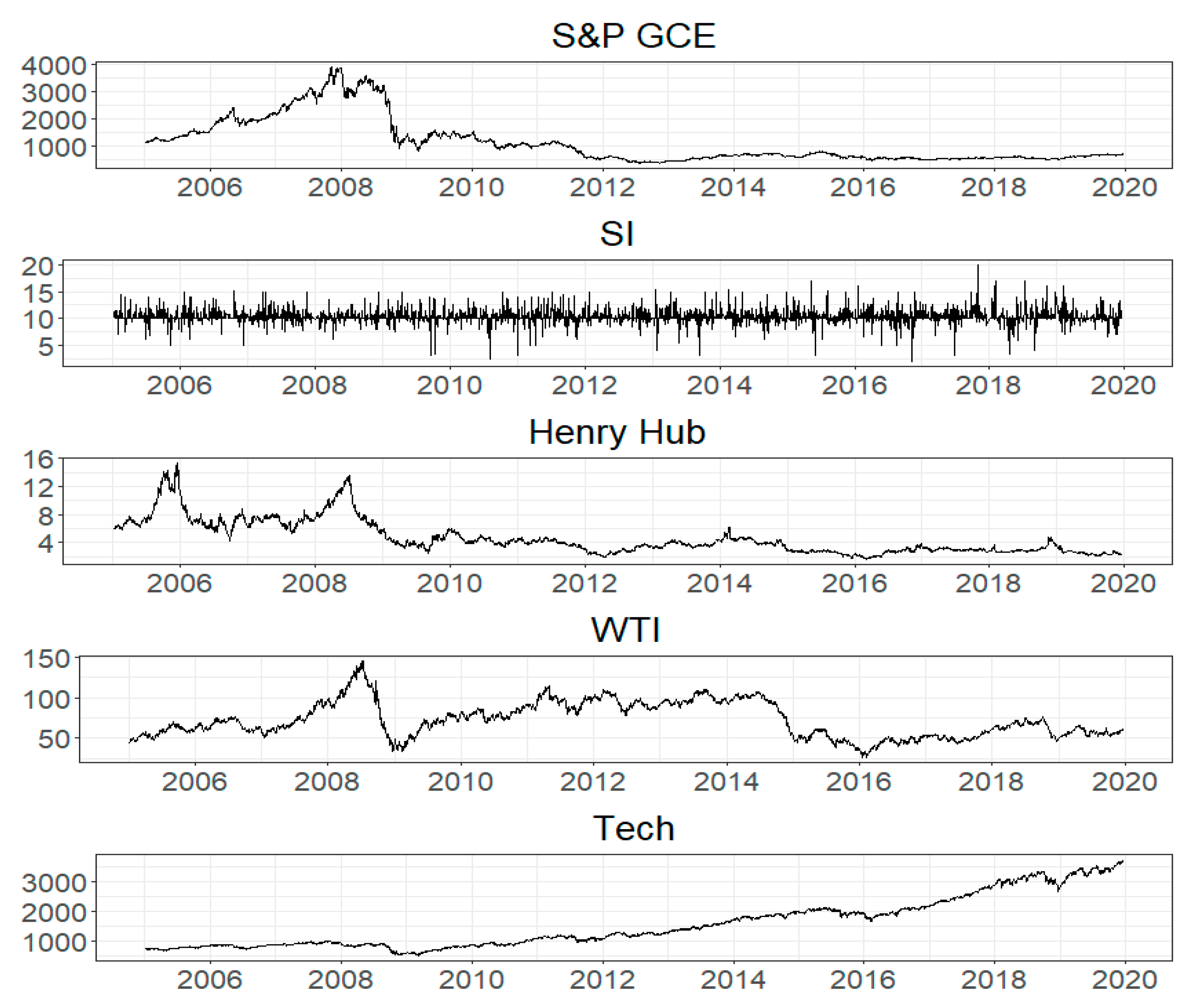
Figure 1. Time variations of variables. Note: S&P GCE, Standard & Poor Global Clean Energy Index; Henry Hub, Henry Hub Natural Gas Futures; WTI, West Texas Intermediate Crude Oil Futures; Tech, NYSE Arca Tech 100 Index; SI, investor sentiment index.
Energies 14 03442 g001
Figure 2. Net pairwise directional return connectedness. Note: S&P GCE, Standard & Poor Global Clean Energy Index; Henry Hub, Henry Hub Natural Gas Futures; WTI, West Texas Intermediate Crude Oil Futures; Tech, NYSE Arca Tech 100 Index; SI, investor sentiment index.
Energies 14 03442 g002
Figure 3. Net pairwise directional volatility connectedness.
Energies 14 03442 g003
Figure 4. Dynamic total return connectedness. Note: the horizontal axis is the timeline; the vertical axis is the connectedness.
Energies 14 03442 g004
Figure 5. Dynamic total return connectedness (TVP-VAR vs. VAR). Note: the horizontal axis is the timeline; the vertical axis is the connectedness.
Energies 14 03442 g005
Figure 6. Time-varying total volatility connectedness. Note: the horizontal axis is the timeline; the vertical axis is the connectedness.
Energies 14 03442 g006
Figure 7. Dynamic total volatility connectedness (TVP-VAR vs. VAR). Note: the horizontal axis is the timeline; the vertical axis is the connectedness.
Energies 14 03442 g007
Figure 8. Dynamic net return connectedness. Note: the horizontal axis is the timeline; the vertical axis is the connectedness.
Energies 14 03442 g008
Figure 9. Dynamic net return connectedness. Note: the horizontal axis is the timeline; the vertical axis is the connectedness.
Energies 14 03442 g009
Table 1. Descriptive statistics of series.
Descriptive Statistics
MeanSkewnessKurtosisJBERSQ (20)Q2 (20)
Descriptive Statistics of the Return
S&P GCE−0.0001−0.2014.2517,323.00 ***−12.37 ***124.95 ***4438.90 ***
Henry Hub−0.00030.7614.8419,463.00 ***−12.67 ***47.42 ***101.87 ***
WTI0.00010.419.616057.50 ***−14.56 ***46.07 ***959.98 ***
Tech0.0005−0.079.185227.30 ***−17.09 ***59.50 ***1803.40 ***
Descriptive Statistics of the Volatility
S&P GCE0.00045.8442.02226,800.00 ***−3.27 ***31,233.00 ***28,301.00 ***
Henry Hub0.00125.7355.31392,012.00 ***−5.22 ***19,180.00 ***10,270.00 ***
WTI0.00064.7433.16136,589.00 ***−4.59 ***31,159.00 ***27,158.00 ***
Tech0.00025.1038.83189,703.00 ***−5.68 ***23,773.00 ***18,520.00 ***
Descriptive Statistics of the Investor Sentiment
SI10.24830.2812.6512,761.00 ***−21.88 ***9.46 ***12.64 ***
Note: JB, Jarque and Bera [28] normality test; ERS, Stock et al. [29] unit root test; Q (20) and Q2 (20), Fisher and Gallagher [30] weighted portmanteau test; *** indicates rejection of null hypothesis at 1% significance level.
Table 2. Average dynamic return connectedness.
S&P GCESIHenry HubWTITechFrom
S&P GCE64.50.51.67.825.735.5
SI0.697.01.00.70.73.0
Henry Hub2.10.890.55.21.49.5
WTI8.80.64.7796.821.0
Tech25.50.60.96.067.033.0
To37.02.58.219.734.6Total: 20.4
Net1.4−0.5−1.3−1.31.6
Note: From, average total directional connectedness received from other variables; To, average total directional connectedness contributed to other variables; Net, average total net connectedness (To–From); and Total, average total connectedness.
Table 3. Average dynamic volatility connectedness.
S&P GCESIHenry HubWTITechFrom
S&P GCE63.11.82.711.620.836.9
SI0.498.40.40.40.51.6
Henry Hub3.70.887.83.64.112.2
WTI9.61.04.373.411.726.6
Tech26.11.82.810.858.541.5
To39.85.310.226.437.1Total: 23.8
Net2.93.7−2.0−0.2−4.5
Note: S&P GCE, Standard & Poor Global Clean Energy Index; Henry Hub, Henry Hub Natural Gas Futures; WTI, West Texas Intermediate Crude Oil Futures; Tech, NYSE Arca Tech 100 Index; SI, investor sentiment index; From, average total directional connectedness received from other variables; To, average total directional connectedness contributed to other variables; Net, average total net connectedness (To–From); and Total, average total connectedness.
Publisher’s Note: MDPI stays neutral with regard to jurisdictional claims in published maps and institutional affiliations.