Review

Velocity Prediction Based on Vehicle Lateral Risk Assessment and Traffic Flow: A Brief Review and Application Examples

1
School of Traffic and Transportation, Northeast Forestry University, Harbin 150040, China
2
Department of Mechanical Engineering, Tarsus University, Tarsus, Mersin 33400, Turkey
3
School of Mechanical and Precision Instrument Engineering, Xi’an University of Technology, Xi’an 710048, China
4
Department of Mechanical Engineering, Texas A&M University, College Station, TX 77840, USA
*
Author to whom correspondence should be addressed.
Energies 2021, 14(12), 3431; https://doi.org/10.3390/en14123431
Submission received: 16 May 2021 / Revised: 6 June 2021 / Accepted: 7 June 2021 / Published: 10 June 2021

Abstract

:
Forecasting future driving conditions such as acceleration, velocity, and driver behaviors can greatly contribute to safety, mobility, and sustainability issues in the development of new energy vehicles (NEVs). In this brief, a review of existing velocity prediction techniques is studied from the perspective of traffic flow and vehicle lateral dynamics for the first time. A classification framework for velocity prediction in NEVs is presented where various state-of-the-art approaches are put forward. Firstly, we investigate road traffic flow models, under which a driving-scenario-based assessment is introduced. Secondly, vehicle speed prediction methods for NEVs are given where an extensive discussion on traffic flow model classification based on traffic big data and artificial intelligence is carried out. Thirdly, the influence of vehicle lateral dynamics and correlation control methods for vehicle speed prediction are reviewed. Suitable applications of each approach are presented according to their characteristics. Future trends and questions in the development of NEVs from different angles are discussed. Finally, different from existing review papers, we introduce application examples, demonstrating the potential applications of the highlighted concepts in next-generation intelligent transportation systems. To sum up, this review not only gives the first comprehensive analysis and review of road traffic network, vehicle handling stability, and velocity prediction strategies, but also indicates possible applications of each method to prospective designers, where researchers and scholars can better choose the right method on velocity prediction in the development of NEVs.

1. Introduction

Today’s world is undergoing unprecedented changes in the 21th century. A new round of technological revolution and industrial transformation is in the ascendant, and intelligent networked new energy vehicles (NEVs) have become the strategic direction of global industrial development [1]. In February 2020, China’s 11 national ministries and commissions, including the National Development and Reform Commission, the Ministry of Industry and Information Technology, the Ministry of Public Security, and the Ministry of Transport, jointly issued the Smart Vehicle Innovation and Development Strategy in its “Strategic Vision”, which points out that: “Looking forward from 2035 to 2050, China’s standard intelligent vehicle system will be fully completed and more complete. The vision of a safe, efficient, green, and civilized intelligent vehicle system has been gradually realized, and the intelligent vehicle can fully meet the people’s growing needs for a better life.”
The application of traffic information in the design of hybrid electric vehicles (HEVs) energy management is one of the important objects, wherein the adjustment of power distribution ratio based on traffic information is achieved by predicting the change of vehicle speed [2,3]. In order to achieve the goals of “safe”, “efficient”, and “green” for future intelligent networked NEVs, it is of great significance to predict and plan their future speed [4,5], because the above three goals are closely related to the speed, as shown in Figure 1. “Efficient” means that the vehicles in the traffic flow move at high speeds, which makes the roads more efficient. A vehicle driving at a higher speed increases the probability of road traffic accidents, so in order to drive “safely”, the vehicle often slows down in advance in the condition of high traffic risk. This process leads to the change of vehicle speed and the problem of optimal vehicle speed planning. Accurate speed prediction is the key to energy management, reduce emissions, and improved energy-saving control of NEVs [6,7], that is, “green” driving. Therefore, it is of great significance to accurately predict and reasonably plan vehicle speed for balancing the relationship among “safe”, “efficient”, and “green” of vehicles in the future traffic system.
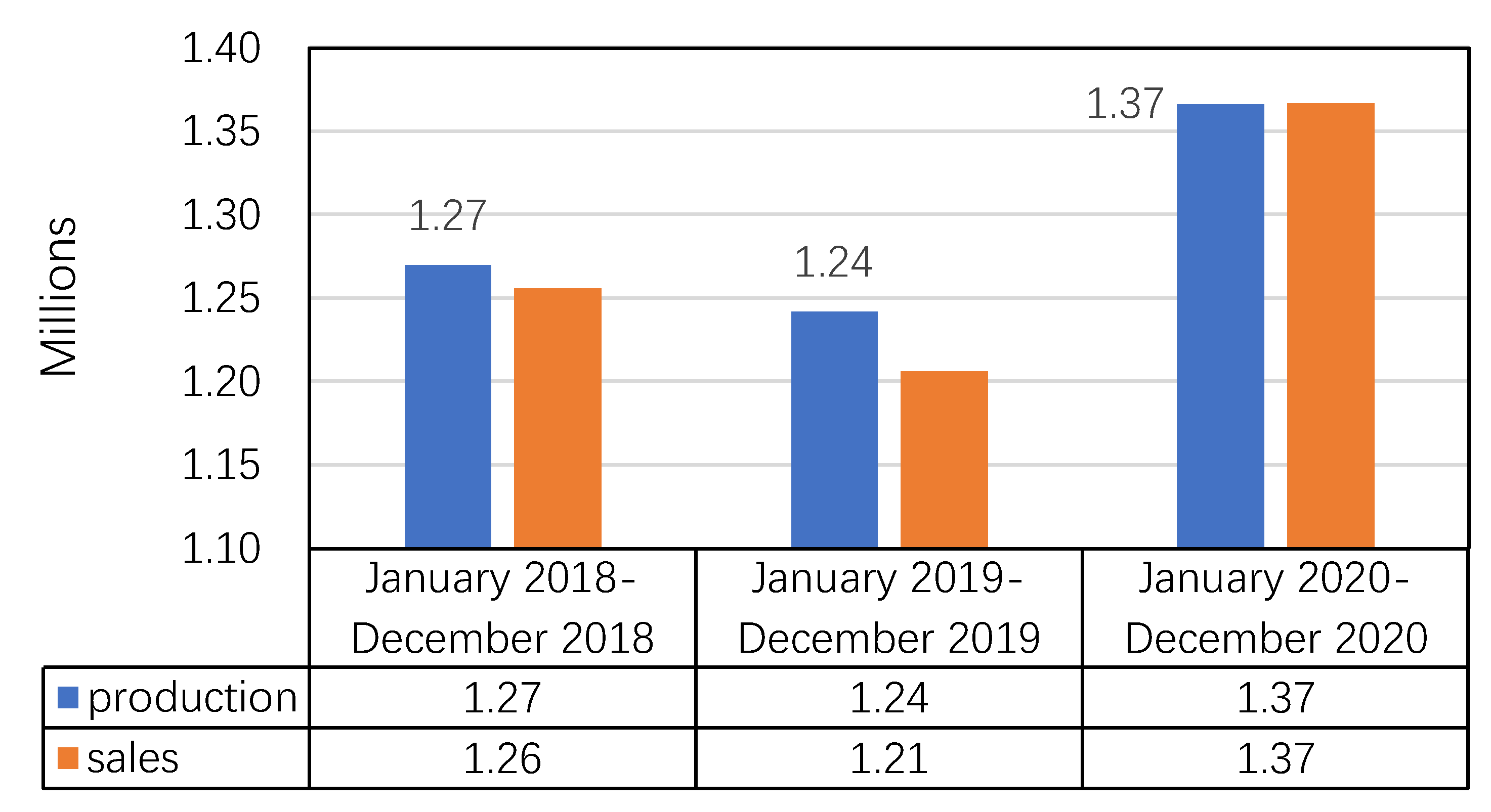
The automobile industry is now undergoing an electrification revolution. Take China as an example, in 2018, the production and sales of NEVs reached 1.27 million and 1.256 million units, respectively. In 2019, the production and sales of NEVs reached 1.242 million units and 1.206 million units, respectively. From January to December in 2020, the production of NEVs reached 1.366 million units, and the sales volume reached 1.367 million units [8].
The above data is briefly described in Figure 2. On the whole, China’s new energy vehicle production and sales are greatly affected by government policy. In 2019, due to the retreat of subsidy policies, the production and sales of NEVs decreased compared with 2018. Due to the impact of the epidemic, China restored the subsidy policy of NEVs in 2020, and the production and sales increased accordingly.

1.1. The Relationship among Velocity Prediction, Traffic Environment, and Vehicle Handling Dynamics

In order to achieve the goals of “fast”, “safe”, and “energy savings” for future intelligent networked NEVs, a basic challenge is to model the road traffic environment and accurately predict the evolution of traffic flow [9]. Accurate speed prediction is the key to energy management and energy-saving control of NEVs, and the driving condition determines the energy consumption and driving safety simultaneously. Therefore, it is very important to predict and select working conditions. Drivers control vehicles’ speed, and in fact interfere with the prediction of the speed. The level of human driving skills plays a key role in the prediction error of longitudinal and lateral speed. In the context of intelligent connected vehicles, a vehicle can automatically perceive the surrounding environment and drive themselves. The vehicle will have a clear understanding of its future traffic environment and its handling stability, which will increase the accuracy of speed prediction. Therefore, the velocity prediction method is based on vehicle dynamics concerned for intelligent and connected NEVs in this paper.
The road traffic network has temporal and spatial, self-organization, and random characteristics. Analyzing the dynamic evolution law of the road traffic network and the traffic operation situation is helpful to fully understand the complex characteristics of the road network, and one can grasp the mechanism of traffic bottlenecks and traffic accidents [10]. The traffic dynamic evolution law model under the mixed traffic network is constructed to realize the rapid identification of traffic behavior characteristics, which provides technical support for further prediction and evaluation of vehicle speed and road traffic network security risks.
Speed prediction is not only related to the inherent characteristics of traffic flow but also related to the judgment of drivers or intelligent vehicles for traffic risks. Combined with intelligent networked vehicles, the road network abstract model and traffic risk prediction and evaluation model with low computational resource occupancy and more flexibility will lay a foundation for vehicle velocity/routing planning technology under multiple constraints and more effective traffic management methods. Therefore, the establishment of a traffic risk prediction and assessment model based on real-time information is of great importance for improving the safety of vehicles driving in bad weather conditions such as rain and snow. How to effectively integrate the existing traffic information collection methods to analyze the evolution law and operating situation of the road traffic network in real-time, and to accurately assess and predict traffic network security risks is a key research topic in the field of road traffic safety [10]. The framework of road traffic network security risk identification is shown in Figure 3.
The safety and reliability of traffic have an important influence on users’ speed choices [11]. Road traffic network safety risk prediction and assessment is a process of accurate identification, effective assessment, and early warning of risks in road network, which is the core link of road traffic network risk identification [10]. Previous studies of road network safety risk assessment are mostly based on traffic accident simulation or later on the basis of traffic accident data analysis and the qualitative assessment, such as road network risk impact factor assessment, road network vulnerability assessment, and vehicle collision risk factor prediction in case of emergency or extreme weather, but it is difficult to find the safety risk impact factors before the accident on time [10]. Traffic hazard identification and risk quantitative assessment before accidents are the key technologies to break through the risk identification of road transportation network [10].
Under bad weather conditions such as rainy and snowy, research on road traffic risk prediction and assessment has a practical significance for vehicle speed forecast and planning. In order to predict traffic risk, it is necessary to explore the evolution law of road traffic system, which is quantified by the traffic flow model. The evaluation of traffic risk needs to be established with the lateral dynamic model and stability controller model of the vehicle. Vehicles with different handling characteristics need a personalized vehicle traffic risk prediction and assessment. Therefore, we will review the influence of various stability control methods on speed prediction. Next, we will introduce the current research progress of macroscopic traffic flow model and artificial intelligence big data model. At the same time, we will explore the tendency of these two-model combined with lateral traffic risk assessment model on the prediction and assessment of traffic risk. It will give a direction of the solution for basic theoretical problems of real-time accurate prediction and assessment of traffic risk before the accident, with the goal of improving vehicle safety and saving energy for the application of safe path and energy-saving speed planning of intelligent networked vehicles.

1.2. Contributions and Paper Structure

Although there are many studies on energy management strategies (EMSs) for HEVs [12,13,14], there is almost no work that has focused on velocity prediction methods combined with traffic risk prediction and assessment of HEVs. In the literature, studies on driving prediction of predictive energy management of plug-in hybrid electric vehicles are put forward [15] without introducing traffic risk prediction and assessment of HEVs.
Thus, the inspiration behind this article is to conduct a brief review on vehicle speed prediction based on traffic environment and vehicle lateral risk assessment. Prospective designers of NEVs will benefit from a number of approaches in the field where they can better establish their solutions. In response to the above analysis, the contributions of this paper are as follows:
(1)
Firstly, we reviewed the macroscopic-traffic-flow-model-based prediction method, which could help improve vehicle speed prediction. This mathematical model has a quick solving speed, and it is easy to integrate the advantages of the information from various traffic sensors and communication systems. This makes the amount of interference quickly back the forecast results in real-time traffic.
(2)
Secondly, we reviewed forecasting method based on traffic data, helping to facilitate the possible integration of multiple prediction algorithms. On combining model-based forecasting methods and data-based forecasting methods, the hybrid prediction method has high computing efficiency, covering more data, and updating online at the same time. This paper can help improve the prediction method’s instantaneity, accuracy, and robustness.
(3)
Thirdly, different from available studies, since the vehicle lateral dynamics and correlation control methods are emerging techniques for velocity prediction, we provide a list of studies for potential applications in velocity prediction in NEVs.
(4)
Fourthly, a questionnaire section about the influence of various traffic flow models and vehicle lateral dynamics is given, and the application field of speed prediction algorithms along with missing points provides deep insight for prospective designers.
(5)
Lastly, a set of application examples are given, wherein three applications are introduced considering various traffic flow models, vehicle lateral dynamics, and speed prediction methods.
This survey is structured as follows. A review of vehicle speed prediction methods for NEVs, with an emphasis on macroscopic traffic flow models, data-based traffic flow models, and influence of vehicle lateral dynamic on speed prediction is introduced in Section 2. In Section 3, research status and analysis of the development of vehicle speed prediction methods for NEVs are established. The application field of speed prediction is discussed in Section 4. Lastly, conclusions and future trends are summarized in Section 5.

2. Review of Vehicle Speed Prediction Methods for NEVs

The velocity of a vehicle is closely related to its traffic environment. Therefore, it is important to accurately predict the change of traffic flow parameters for improving the accuracy of vehicle speed prediction. We now introduce macroscopic traffic flow models, data-based traffic flow models, and the influence of vehicle lateral dynamics on speed prediction in this sequel.

2.1. Macroscopic Traffic Flow Model and Vehicle Velocity Prediction

Macroscopic traffic flow models use a mathematical model to describe traffic dynamics. The mathematical model evaluates the unmeasured area based on real-time input data. This model is usually based on empirical relationship, in which the parameters to be evaluated are either obtained from external calculation of historical data or generated from internal evaluation of an algorithm. The macroscopic traffic flow model method has been widely used in traffic state assessment.
Literature [16,17] introduces in detail the current developments and trends of the above macro traffic flow model, as well as traffic modeling, evaluation, and control methods based on intelligent networked vehicles. The macroscopic traffic flow model method has the following advantages: First, this method explains the mechanism of traffic, expands the observation data, and provides additional information. Therefore, this method can use less data to predict accurate traffic conditions. Second, it has higher interpretability. This means that even if the prediction is not accurate, the reason may be found in a certain confidence interval. Third, it can be directly integrated with traffic control practices, such as using model predictive control. The macroscopic traffic flow model method also has the following shortcomings: First, inaccurate or uncalibrated models will lead to poor performance of traffic state assessment results. Therefore, in actual application, the macroscopic traffic flow model traffic state assessment method must be carefully selected and calibrated. In this case, checking the validity of a model or calibrating a model requires a big set of data [18]. Second, since the macro-traffic flow model cannot be adjusted adaptively, it cannot reflect the changes in traffic flow brought by random traffic interference alone. Therefore, in the absence of real-time traffic information, it is more suitable for the prediction of traffic flow that does not change rapidly, such as the prediction of traffic parameters in expressways and urban loops.
Traffic flow (simulation) models are used to characterize complex traffic flow systems in order to understand, describe, and predict traffic flow [19]. It is a basic tool for analysis and experimental research of transportation systems. The traffic flow model is not only used in the traditional fields of traffic system design, testing, management, and personnel training. With hot research direction on intelligent vehicles and intelligent transportation systems, it has also been used to evaluate and predict the state of the transportation system [18]. Macroscopic traffic flow models can be classified according to the degree of detail they represent in traffic systems. This classification can be implemented by considering different levels of traffic entities in their respective flow models. Literature [20] classifies the traffic flow model as follows:
  • Submicroscopic models (describing in detail the equations of vehicle subunits and their interactions with surrounding vehicles).
  • Micro model (describing the distinction and tracking of individual entities in detail).
  • Mesoscopic model (medium detail description).
  • Macro model (less description of individuals).
The microscopic traffic flow model not only describes the time and space behavior of system entities (vehicles, drivers, etc.), but also describes the interaction between them in detail. For example, a lane change behavior of each vehicle in the flow is described as a series of driver decisions.
Similar to the microscopic model, the submicroscopic model describes the characteristics of a single vehicle in the traffic flow. However, in addition to the detailed description of the driving behavior, the control behaviors (transmission shifting, ESP, etc.) of the vehicle in response to the surrounding conditions are also modeled. Moreover, the sub-modules of the vehicle are also modeled by mathematical equations.
The mesoscopic traffic flow model neither identifies nor tracks individual vehicles, but it lists the behavior of individual vehicles (for example, in the form of probability). In view of this, traffic is represented by small groups of traffic entities. The model does not describe the behavior and interaction of these groups in detail. For example, the lane change of a single-vehicle is described as a transient event. The decision to change lanes is based on parameters such as the relative density of the lane and the speed difference. Some mesoscopic models analogous to the theory of gas motion have been pushed out. These gas motion models describe the dynamic distribution of model velocity.
The macroscopic traffic flow model describes the traffic flow at an overall level without identifying its constituent details. For example, traffic flow is aggregated (represented by flow, density, and speed). The behavior of individual vehicles (lane changes, etc.) is usually not displayed. A macroscopic traffic flow model assumes that it is appropriately allocated to the road lanes and uses approximate methods to achieve it. Macroscopic traffic flow models are usually classified based on the number of their partial differential equations. Usually, one side of the equation is the model representation, and the other side is the order of the equation. Here are some typical traffic flow models and their extended models [18].

2.1.1. One-Dimensional Flow Model

The Lighthill-Whitham-Richards (LWR) model [21] is a famous innovation in the mesoscopic traffic flow model. It uses a conservation law of vehicles in the traffic flow and assumes that the traffic parameters (traffic speed and density) follow a fundamental diagram (FD) in equilibrium. This traffic model has the ability to identify traffic congestion and distinguish between traffic congestion and free flow. Moreover, because of its relatively simple equations, it can be quickly calculated and solved. However, due to the limitations of the model, it cannot reproduce some complicated phenomena, for example: unstable flow and the stop-and-go phenomenon.
After the LWR model, higher-order models were developed in order to show phenomena different from equilibrium traffic state (usually referred to as micro disturbance and non-equilibrium state), higher-order models usually use another momentum equation to describe the evolutionary relationship of traffic speed instead of the FD. The Payne-Whitham (PW) model [22] is the first well-known high-order modeling attempt. The PW model and its extension [23] successfully reproduce some well-known traffic phenomena, such as hysteresis, reduced capacity. However, it still has some shortcomings, such as negative speed [17].
The Aw-Rascle-Zhang (ARZ) model [24] is another high-order model. It allows the equilibrium state of traffic to be transformed into other states. It also overcomes the limitations of the PW model. It can be derived from the LWR model. The ARZ model is further developed and extended to the following models: general second-order model [25], phase change model [26], and generalized ARZ (GARZ) model [27].
Recently, the theory of explaining the traffic flow model has made new progress. Some models can be represented using Hamilton-Jacobi partial differential equations (HJ-PDE). HJ-PDE has been studied in detail in the field of partial differential equations and physics [28], and its theory can effectively solve this kind of model [29]. For example, the traffic density state variable ρ ( t ,   x ) of the traditional LWR model can be transformed into the state variable N(t, x) of the accumulation flow. In addition, due to the nature of the accumulated flow, this model can implicitly express vehicle trajectory and travel time. The relationship between macro and micro can be shown. Then, a Lagrangian coordinate system was proposed and used accumulated flow and vehicle trajectories in the mesoscopic traffic flow model [30]. Similar topics have also been discussed in other traffic flow models [31].

2.1.2. Multi-Lane Models, Multi-Class Models, and Random Models

Actual traffic often has multiple lanes and multiple categories, different from the model introduced in Section 2.1.1. The studies [32,33] proposed some models that consider multi-lane and multi-category traffic behavior. For these extended models, modeling lane change behavior is one of their main challenges. Regarding lane changes, human behavior is quite important.
For the random properties of the traffic and the uncertainty of input/output data, a stochastic model [34] based on the LWR model is proposed. In the references [35,36], the source of randomness in dynamics explains the heterogeneity of vehicles, which means the relationship between multi-class models and random models. Moreover, the work [37] developed an LWR stochastic model based on HJ PDE.

2.1.3. Development Trend

The traffic flow model is not only used in the traditional fields of traffic system design, testing, management, and personnel training [20]. As the research on intelligent vehicles and intelligent transportation systems is a hotspot, it is also used to evaluate and predict the state of the transportation system [18]. It extends from ensuring the stability and energy efficiency optimization of a single vehicle to the safety and efficiency of the entire system.
The main principle of the prediction algorithm is to combine numerical simulation, traffic model, real-time data, and historical data to predict the evolution of future traffic conditions. Designing a fast, scalable, and accurate road traffic forecasting tool is the key to overcome the lack of forecasting ability of the existing traffic management information system [18], and it can be applied to the prediction and planning of vehicle path and speed in the future. At present, there is no hybrid traffic flow model that combines the advantages of macro traffic flow model and data-based traffic flow model. The hybrid traffic flow model is of great significance to improve the accuracy, robustness, and real-time performance of prediction. In the future, the traffic flow model will not be used individually, but a multi-layered hybrid model, as well as possible complementary and combined use of model-based traffic flow models and data-based learning models.

2.2. Data-Based Traffic Flow Model and Vehicle Velocity Prediction

Traffic parameter prediction method based on big data and machine learning has attracted the research interest of many scholars in recent years [38,39]. The traffic management department realizes the prediction of traffic flow by collecting and analysising the current and historical traffic data. Big data analysis can effectively predict the occurrence of traffic accidents. Big data analysis mainly solves the following three problems: data storage, data analysis, and data management [40]. The collected traffic big data is trained into a prediction model by machine learning method to analyze the evolution trend of traffic. Machine learning models can be divided into: supervised learning, unsupervised learning, reinforcement learning, deep learning and entity-based algorithms [40]. The labeled training data is used for supervised learning algorithms. Linear regression, decision tree, neural network and support vector machine are typical supervised learning methods.
The data-based traffic flow model can be divided into historical data-based traffic flow model and real-time big data-based traffic flow model. Among them, the traffic condition assessment method that widely relies on historical data uses a statistical method or machine learning method to find the relationship between historical data. Traffic conditions are evaluated based on this correlation and real-time data, meaning that it does not require prior knowledge of explicit modeling in the macroscopic traffic flow model. This method usually requires a big amount of historical data.
The traffic flow model based on historical data has the following advantage: less time for model selection and calibration. The disadvantages are: first, based on historical data means that the model may fail when unexpected events occur or when a relatively long trend is predicted. Second, the computational consumption required for training and learning will be very high. Third, the method can be regarded as a “black box”, which means it is unable to properly explain the model decisions [18]. Fourth, if the information from real traffic flow is greatly different from that stored in the data used for the training model, the prediction accuracy will not be guaranteed.
Compared with the macro traffic flow model and the traffic flow model method based on historical data, the method based on real-time big data is defined as a method that does not rely on the empirical relationship that appears in the macro traffic flow model but depends on real-time data flow. This means that this method relies less on the prior knowledge of transportation. Its advantage is that it is robust to uncertain phenomena or unpredictable accidents. In an era of ubiquitous sensors (smart phones) and the emergence of a large number of intelligent networked vehicles, methods based on real-time big data streams may become popular in the future [41,42]. This method is more suitable for the prediction of urban road network traffic flow.

2.2.1. Research Status of Traffic Flow Evolution Using History Traffic Data and Artificial Intelligence Methods

It has become a hot research direction using deep learning method to predict the change of traffic parameters, for example in [43,44,45,46,47]. The unsupervised incremental machine learning, deep learning, and deep reinforcement learning was adopted by Dinithi Nallaperuma et al. to structure an expansive smart traffic management platform [43]. It can successfully model traffic flow with fluctuation; however, the method proposed in the literature is not effective for predicting traffic flow with high frequency fluctuation. An improvement to this problem is to increase the amount of data used to train the deep learning model. The restricted Boltzmann Machine method was used to predict traffic [44]. This method has a better nonlinear fitting ability and high prediction accuracy for typical chaotic time series. Di Zang et al. [45] solved the task of long-term traffic speed prediction for elevated highways by coupling convolutional long-short-term memory and convolutional neural network (CNN) into a single framework.
For the problem of uncertain data used in the training model, a common solution is to combine fuzzy rules with deep learning [48] and neural network [49]. By introducing the fuzzy representation into the deep learning model to lessen the impact of data uncertainty, a deep convolutional network model was established to explore the spatiotemporal connection of traffic flow to promote traffic flow prediction in [48]. The experimental results show that the combination of deep learning and fuzzy theory can improve the prediction accuracy, compared with other methods, such as autoregressive integrated moving average (ARIMA), deep learning-based prediction model for Spatial-Temporal data, CNN, fully convolutional neutral network, and fatigue detection convolutional network. The Takagi-Sugeno system was used for fuzzy reasoning, and two learning processes were proposed to update the membership function of the fuzzy system [49]. The proposed method has advantages over the six traditional models, such as artificial neural network, support vector machine, ARIMA model, and vector autoregressive model.
In addition to representing uncertainty with fuzzy rules, another approach is to point out exactly what the uncertainties are and then label those uncertainties with contextual factors. The relationship between traffic flow values in a time interval is investigated based on a combination of contextual factors from historical data [50]. From the analysis results, forecasting accuracy can be better improved by the proposed new method. On the other hand, the design is slightly inferior to the conventional method due to inconsistent points. This can be interpreted to the high volatility degree associated with low-traffic-flow periods.
There are several ways to improve the prediction accuracy of deep learning methods: training data are screened [51,52] or training parameters are optimized [53]. A deep belief network (DBN) model and a kernel extreme learning machine classifier is combined as a prediction model, wherein the important features of the traffic flow data are extracted through DBN at the bottom of the network. To predict the traffic flow, the extracted results are inputted into the kernel extreme learning machine classifier [52]. Automatically use those highly correlated spatiotemporal points to train the deep learning network, and reduce the use of less correlated data [51]. This explains the interaction between past and future data to some extent. Traffic flow theory and its application on urban transportation networks with more efficient deep learning architectures is a promising study field [51]. This is the valuable research direction recommended by this paper.

2.2.2. Research Status of Velocity Prediction Using Real-Time Traffic Data

Real-time prediction model of vehicle travel speed is helpful to improve vehicle safety, maneuverability, and fuel economy. In order to achieve these effects, an accurate velocity prediction model needs to be established and can be successfully implemented in the real system. There are two main types of vehicle speed prediction models: the prediction model based on Markov chain and the prediction model based on recursive neural network. Markov chains are stochastic data-driven models that predict future states from state transition matrices and current states. Transient probabilities are aggregated into state transition matrices. The structure of measurement based on transfer conditions is intuitive and easy to implement. There are three kinds of Markov chain models: interval coding, fuzzy coding, and velocity constraint model [54]. The speed prediction models are based on recurrent neutral network (RNN) including standard RNN, long short-term memory, and gated recurrent unit (GRU) models [54]. Among the three models based on Markov chain, the model combining the fuzzy coding method and the constraint model has the highest prediction accuracy. Of the three RNN-based models, GRU has the highest prediction accuracy due to the appropriate structure of long-term dependent learning by combining the amount of previously determined state data [54].

2.2.3. Development Trend

More research study needs to be performed in the following aspects for future data-based vehicle speed prediction methods [15]:
  • Multiple prediction algorithms integration.
  • Online correction and update technique.
  • Balance between running online and computing burdens.
  • Driver model and driving style recognition.
  • Multi-source information integration.

2.3. Influence of Vehicle Lateral Dynamic on Speed Prediction

The influence of vehicle lateral dynamics on vehicle speed prediction is based on the traffic risk assessment from drivers or intelligent vehicles. Traffic risk assessment models can be divided into two types: longitudinal and lateral models. The longitudinal traffic risk assessment model mainly evaluates vehicle collision accidents caused by untimely braking or insufficient braking force. It includes a risk assessment model based on traffic accident data or simulation data [55,56] and a model-based risk assessment model [57,58,59]. Model-based work often requires parameters and empirical assumptions, while data-based methods only focus on extracting the relationship between images and road safety without considering other influencing factors such as drivers; thus, it has certain limitations.
Lateral traffic risk assessment models often build lane change risk models based on road traffic environment and lane change path factors, such as building a highway exit lane change risk model based on a proportional advantage model [60]. The existing literature rarely considers the impact of the traffic environment and vehicle lateral handling characteristics [61]. How to dynamically and accurately analyze the impact of traffic conditions on the prediction of vehicle velocity change and intermittent road safety (vehicle lateral stability) is a huge challenge for road safety analysis in practical application [60].
In order to study the stability characteristics of different vehicles and generate their stability criteria (lateral traffic risk assessment model), it is necessary to study the structural characteristics of vehicles and their handling stability control methods. For example, distributed drive control (also known as torque vector control) enhances the vehicle’s dynamic performance [62], so its traffic risk assessment should be different from that of ordinary front-wheel steering vehicles. In a similar work, Kun jiang et al. [63] presented a method to estimate and predict individual tire forces based on a vehicle dynamics model and observer with low-cost sensors and driver assistance map, which is in close relation to the speed of the vehicle. Yu-Chen Lin et al. [64] developed an ecological cruise control based on an adaptive prediction-based control strategy. The design guarantees the safety of driving, riding comfort, as well as fuel efficiency simultaneously when running on roads with curves and up-down slopes. However, the above two literature did not involve the personalized assessment of vehicle traffic risk, nor did they pay attention to the relationship between traffic risk and predicted speed.
Some researches combine vehicle lateral safety with longitudinal speed prediction. To this end, a three-degree-of-freedom vehicle lateral dynamics model with lateral load transfer ratio index is derived for a rollover speed prediction model in [65]; similarly [66,67]. Lin Li et al. [68] combined the energy management of HEVs with vehicle speed prediction and planning before entering the corner. Pan Song et al. [69] demonstrated an improved optimal speed adjusting method based on the vehicle handling stability and path following performance. Med Krid et al. [70] presented a model predictive control (MPC) strategy for an active anti-roll system, which aims to minimize the load transfer during cornering and the consumed energy by the actuators. Hongbin Ren et al. [71] formulated a quadratic optimization problem for an integrated control of longitudinal speed and lateral motion control based on longitudinal progression maximization and lateral path tracking error minimization.

2.3.1. Influence of Vehicle Stability Control Methods on Speed Prediction

In order to reach the destination faster, the driver or the intelligently connected vehicles will choose a higher speed, which means that the vehicle’s speed is greater than the speed of the surrounding vehicles (traffic), so it needs to overtake and change lanes frequently. In bad weather conditions such as rain and snow, this can bring the risk of accidents such as vehicle skidding. Moreover, in a cold region’s road traffic environment, traffic accidents caused by overtaking and lane change on snow and ice slippery road surface are common. In addition, vehicle steering characteristics, driving characteristics, control methods, mass, the height of center of mass, wheelbase, tire lateral stiffness, and other factors affect vehicle handling characteristics in a road traffic environment. Therefore, in order to assess the traffic risk caused by sideslipping and predict the speed variation of the vehicle, a method of lateral traffic risk assessment and speed prediction based on vehicle handling characteristics should be established. This lies in the connection between personalized lateral traffic risk assessment demand and vehicle speed prediction demand. Analyzing the mechanism of mutual coupling between the two demands is beneficial to improve the accuracy of risk assessment prediction and vehicle speed prediction at the same time, so as to achieve the goal of improving road traffic safety and energy saving.
Modern vehicles are equipped with advanced vehicle lateral control strategies, such as active front steering (AFS) and direct yaw moment control (DYC) to enhance vehicle lateral motion control. In recent years, there have been continuous publications on vehicle lateral dynamics control, such as [72,73,74]. At present, the research literature on distributed electric drive is limited, and it mainly focuses on the theme of four wheel independently actuated electric vehicle. The research content mainly focused on the innovation and application of control methods, such as [75,76,77]. The uncertainty of tire-road friction factor and vehicle load distribution affect the lateral stability and handling performance of the vehicle. The vehicle dynamics solution for this problem is through a combination of active rear wheel steering (ARS) (also known as “four-wheel steering”) and DYC, or through AFS combined with DYC. The study [78] proposed a cooperative control method of AFS and DYC based on optimal guaranteed performance to achieve stability and better vehicle maneuverability. Literature [79] considered the lateral dynamics stability of the vehicle under the condition of time-varying vehicle longitudinal speed. In the work [80], an augmented linear variable parameter model based on combined proportional integral control rate and a robust gain-scheduling state-feedback controller is proposed. It minimizes the energy-to-peak control performance of the AFS/DYC system. Other researchers have proposed the combination of front-wheel active steering and direct yaw moment control to promote vehicle handling and stability in the literature [81]. The innovation of the above control methods focuses on the vehicle, closely following the reference path in the interference environment, but the speed prediction problem is not studied. Studies that combine speed prediction with vehicle lateral dynamics are usually found in driving decision problems, such as [82]. A receding horizon method based on mixed logic dynamics constraints with the objectives of the steering wheel of the driver, longitudinal speed control, and lateral lane tracking performance is established through a safety-guaranteed optimization model.

2.3.2. Development Trend

There is no control strategy to restore the stability of a vehicle after the tire forces on all four wheels are saturated, because there are no more controllable external forces acting on the vehicle. In this case, the way to avoid danger is to anticipate the danger in advance and take actions to avoid it. This is reflected in advance during the deceleration of vehicles, that is, the “speed prediction and planning” mentioned above. Therefore, it can be said that accurate prediction and planning of vehicle speed is very important for both vehicle energy efficiency and vehicle handling stability.
The existing distributed drive control theory research mainly focuses on the four-wheel independent control of electric vehicles. As the degree of vehicle electrification increases, there will be more and more research on the comprehensive consideration of distributed drive control and energy management of hybrid vehicles [65].
The advantages, disadvantages, and applications of the above traffic velocity and vehicle speed forecasting methods are shown in Table 1.

2.4. The Relationship between Energy Management and Velocity Prediction of HEVs

The United States Energy Information Administration forecasts that oil and other liquid fuels will continue to dominate the transportation industry from 2010 to 2040 although it is noted that their share will decrease significantly (for example, from 98% to 80%) [83]. In other words, fossil energy will still be the main energy resource under the current situation that diesel vehicles account for the majority. Carbon dioxide emissions produced by the transportation industry account for 22% of all emissions, which leads to climate change issues such as global warming [84]. To address air pollution, climate change, and energy shortages, vehicle engineering researchers and policymakers are looking for sustainable alternatives that are less dependent on oil and cause less pollution. HEVs is one of the most promising alternatives.
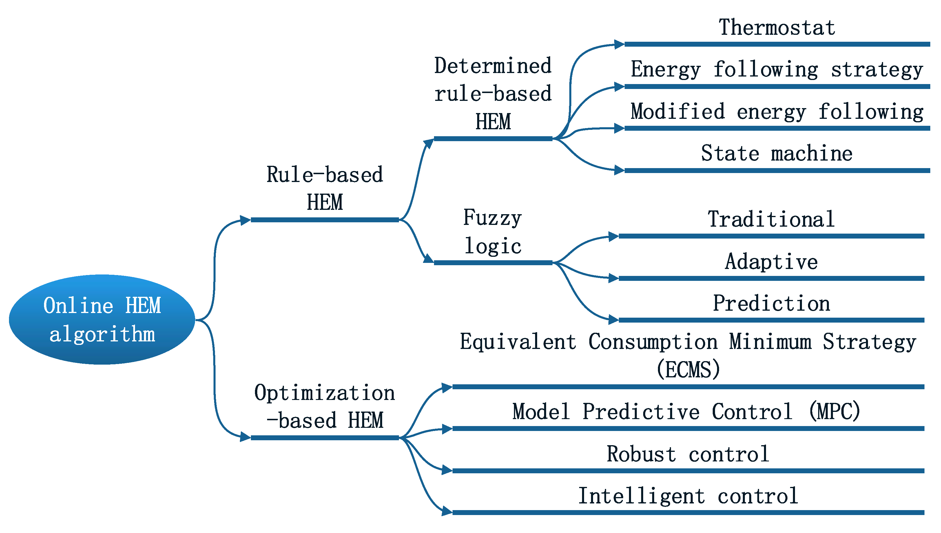
The main purpose of energy management is to allocate energy demand among different energy sources in order to maintain battery state-of-charge (SoC), optimize energy efficiency, and reduce fuel consumption and emissions, among other related purposes. Huang, Y. et al. [85] divides energy management strategies into two categories: offline and online. The benchmark for this classification is whether the algorithm can operate in real-time, because energy management is designed to be applied in real-time, or as a benchmark to prove the effectiveness of other approaches. Online energy management algorithms can be divided into rule-based energy management and optimization-based energy management [85], as shown in Figure 4.
Velocity prediction and the quality of prediction results have great impacts on the performance of corresponding predictive energy management strategies (PEMSs) [15]. Velocity prediction should pay attention not only to the accuracy of the prediction, but also the length of the forecast time.

2.4.1. The Accuracy of Velocity Prediction in the Effectiveness of Energy Management

It is common to study an improved velocity prediction in the existing energy management methods of HEVs. Velocity prediction is usually associated with hybrid systems to achieve the objectives of minimum energy consumption, increasing battery life, improving driving safety, etc. Typical examples are given below:
A driver-oriented velocity prediction is created by a deep fuzzy predictor utilizing fuzzy granulation technology, and vehicle speed and acceleration are learned by transition probabilities of a finite-state Markov chain. A chaos-enhanced accelerated swarm optimization is presented with the dual-loop online intelligent algorithm to optimally determine power distribution between two power sources [86]. Markov chain and fuzzy C-means clustering are proposed for cooperative velocity forecasting that is composed of predictive sub-models to deal with various driving patterns. Forecasted velocity profiles are blended via the entire sub-models using quantified fuzzy membership degrees to obtain the final prediction results [87].
Under different short-term velocity horizons, i.e., 5 s, 10 s, and 15 s horizons, a deep neural network is utilized. At the same time, to calculate the optimal power-split at each MPC decision step, the dynamic programming method is applied [88]. Another strategy to speed forecast is introduced via a multi-stage neural network in [89]. ARIMA (autoregressive integrated moving average)-based data-driven strategy to predict short-term speed and road gradient in real-time is demonstrated [90].
Based on the driving power distribution under different driving cycles, a reinforcement learning controller (RLC) trained by the Q-learning algorithm is studied. A multi-step Markov speed prediction model-based RLC is embedded into a stochastic MPC to find optimal battery power in the predicted time [91]. To achieve the cross-type knowledge transfer between deep learning-based EMSs, a transfer-learning-based method is designed [92].
Another method is the pattern sequence-based speed predictor for accurate short-term speed prediction [93]. It is important to highlight that there are numerous speed prediction strategies based on the driver model. The main idea is that the speed prediction is obtained with optimization of the engine torque, the brake force, and the gearshift schedule, taking into account safe driving distance and traffic speed limits [94].
Through literature research, it can be concluded that accurate speed prediction can improve the above-mentioned objectives. The objective of speed planning and energy management is generally conflicted with driving safety cost, energy consumption cost, and battery life loss when the EMS is defined as a co-optimization problem over the moving horizon [95]. To better understand the influence of horizon length in speed prediction, the following section is introduced.

2.4.2. The Time Length of Velocity Prediction

For the prediction length of traffic parameters, it is relatively easy to accurately predict the change of traffic parameters within a short period of time, because the existing literature assumes that the traffic parameters remain unchanged within a short period of time [15]. However, short-term prediction of traffic parameters has limitations in practical application. For example, when short speed prediction is applied to the energy management of HEVs, it will lead to suboptimality of the solution [15]. In addition, short-term traffic parameter prediction cannot adequately provide the information required for vehicle path planning, and incorrect path planning will lead to the complete loss of fuel economy improved by predicted energy management [15].
These are the current challenges in accurately predicting traffic parameters: (1) The contradiction between prediction accuracy and computation burden (for example, the number of parameters to identify past traffic flow segments); (2) How to choose the duration of data collection and traffic parameter prediction so as to balance the contradiction between prediction accuracy and application requirements?

2.4.3. Development Trends

The goals of energy management for hybrid vehicles are as follows [65]:
  • The engine operates in an efficient range.
  • Making the vehicle friction process (between the tire and the road, and friction braking) as little as possible.
  • Increasing battery life. Battery SoC is not too high or too low (usually between 40% and 90%), and corresponds to saturated (90% to 100%) and insufficient (0% to 40%) states.
The second goal is the core issue of vehicle energy management, that is the “speed forecast and planning” that should be as accurate as possible in the future. The goal of “speed forecast and planning” is not limited to individual vehicles, but should be extended to the entire transportation system. In future, vehicular communication networks (vehicle-to-everything (V2X)), i.e., internet of vehicles and traffic infrastructure (mainly referring to traffic sensors, communication network, and big data analysis and prediction), should be established, and improvements should be made in vehicle intelligence vehicle electrification—braking should be mainly completed by regenerative braking of the motor. One goal of NEVs is to focus on braking without the frequent use of brakes, that is, to pursue accurate prediction and planning speed. Braking is only used in case of emergency.

3. Questions Raised

From the above research status and development analysis, the following key issues need to be resolved urgently: (1) Establishing a mixed traffic flow model to measure the overall operation of the comprehensive transportation network. The mixed traffic flow model is a complex transportation system model that breaks through the traditional single road network level and integrates multiple types of road networks. (2) Most safety risk assessments are based on accident data analysis, and the identification and quantitative assessment of risk points before accidents need to be improved. At the same time, the vehicle speed prediction method based on vehicle lateral dynamics needs to be studied carefully. Therefore, it is an interesting research direction to study the vehicle speed prediction method, which integrates vehicle handling stability and mixed traffic flow model with its mechanism and implementation method for improving vehicle safety and energy savings. It will have an important impact on improving traffic efficiency, reducing traffic risks, and improving energy utilization on a theoretical basis, revealing the dynamic evolution law and traffic operation situation of road traffic network, mastering the formation mechanism of traffic bottlenecks and traffic accidents. Further, the safety risk of road traffic network needs to be evaluated, so as to lay the foundation for early prediction and avoidance of accidents under adverse weather conditions such as rain and snow. In terms of practical engineering applications, the results provide personalized traffic risk assessment for vehicles with dynamic and handling characteristics, which can improve vehicle safety (safe path planning method) and energy utilization efficiency (energy-saving speed planning method), and promote the application and market-oriented development of intelligent vehicles and intelligent transportation systems.

3.1. Traffic Flow Model (Both Macro and Data-Based)

The macroscopic traffic flow model has experienced a relatively long period of development, and it is still continuing. In recent years, machine learning methods have been used to study and predict traffic parameters. Both model-based and data-based traffic flow models have their own advantages. Their comparison and possible combination and complementarity will be a research direction in the future.
For macroscopic traffic flow models, the following questions need to be answered:
  • What causes errors in the macro traffic flow model?
  • What determines the magnitude of the error?
  • How to improve the model to reduce the error?
  • What is the cause of the error in the prediction delay in the time axis?
For data-based traffic flow models, we have the following questions:
  • How does the macroscopic traffic flow model and the data-based model affect the error of prediction results?
  • How can combining the above two methods reduce prediction error?
  • How can neural networks correct the prediction delay of macroscopic traffic flow models?

3.2. Influence of Vehicle Lateral Dynamic on Speed Prediction

For the influence of vehicle lateral dynamic on speed prediction, we have the following questions:
  • What are the vehicle handling stability factors causing the speed prediction error?
  • How do traffic velocity and traffic density affect drivers’ decision-making with different handling characteristics?
  • Energy, time, and safety are often conflicted. Their weights vary depending on the driver. What is the mechanism by which we get optimal path and speed?
  • Planning the longitudinal speed of intelligent vehicles to improve traffic efficiency, traffic safety, and energy utilization efficiency is a key scientific problem.

4. The Application Field of Speed Prediction

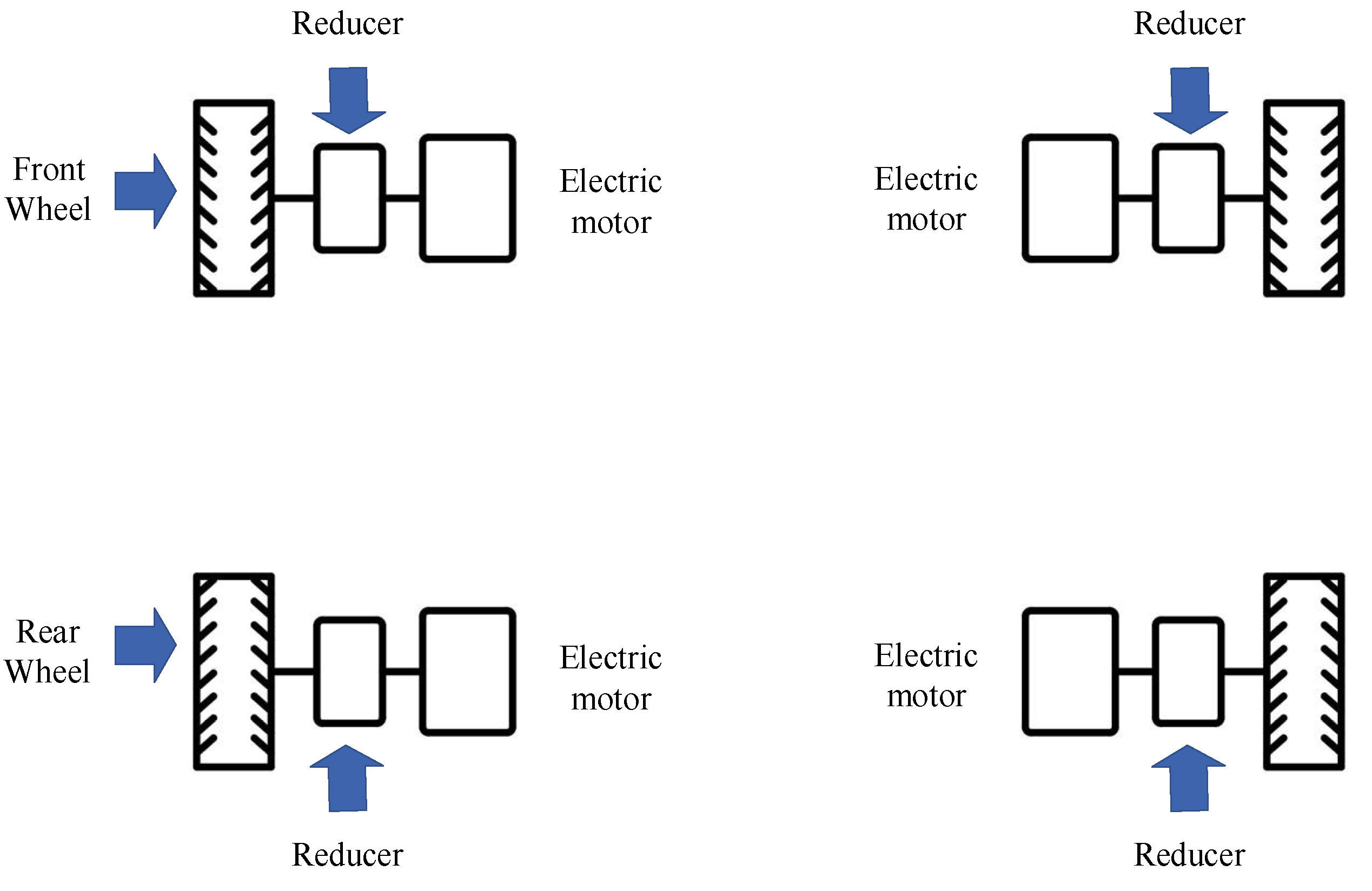
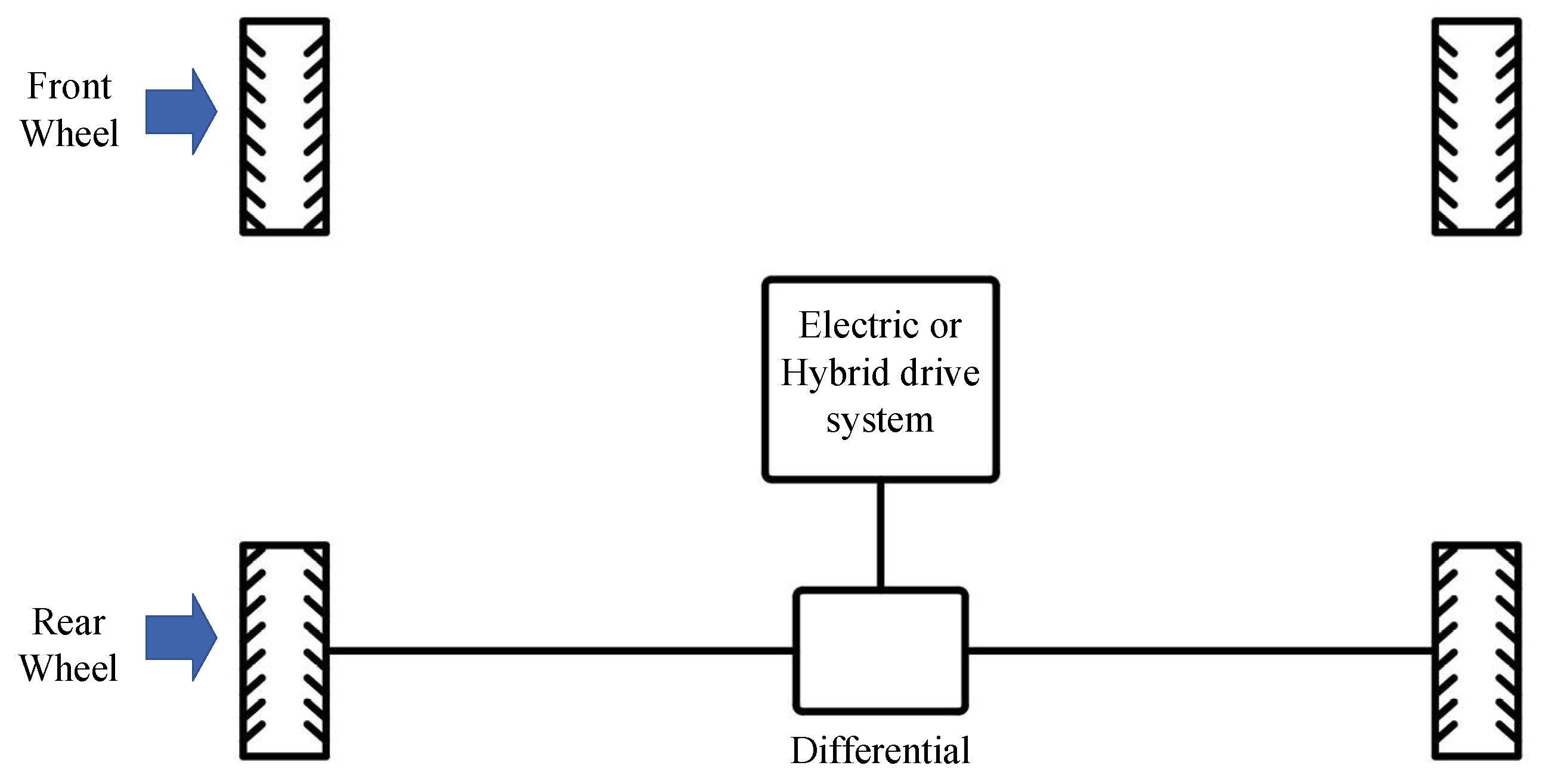
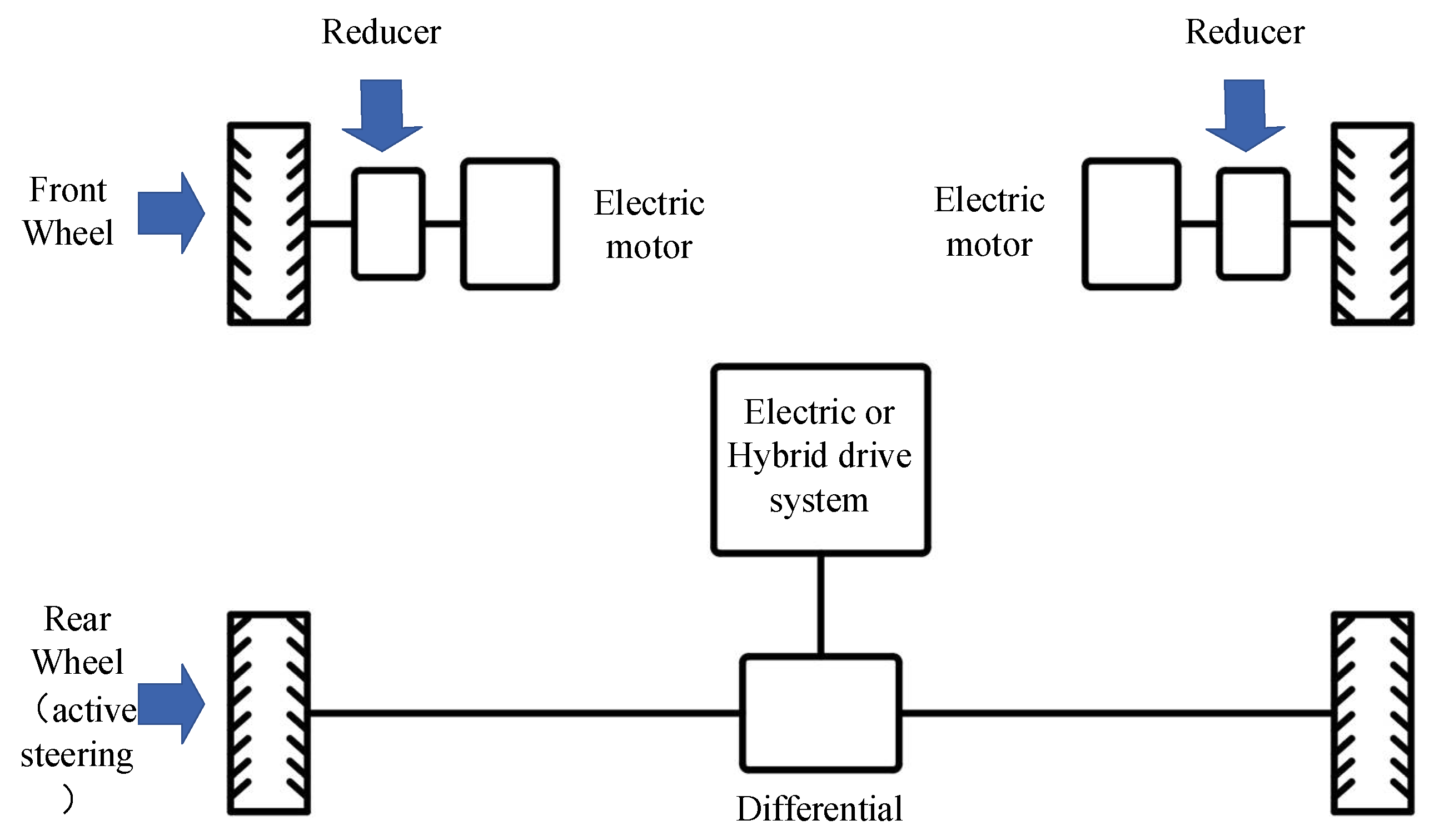
The development of modern intelligent vehicles and intelligent transportation systems requires that different research directions in the past be integrated and comprehensively considered to meet the requirements of simultaneous realization of multiple goals in vehicle design and transportation fields. The comprehensive consideration of vehicle “lateral handling stability” and “optimal energy efficiency” is becoming a trend. The power and steering structures of the existing NEVs are shown as Figure 5, Figure 6 and Figure 7. The existing literature mainly focuses on the optimal multi-objective control problem of the handling stability and energy efficiency of pure electric vehicles [96,97], and its structure is shown in Figure 5. Energy management studies are common in the design of HEVs, for example: [98]. The stability control of HEV is usually obtained from a series hybrid vehicle similar to the four-wheel independent drive pure electric vehicle, for example: [99]. However, the optimal multi-objective control problem of handling stability and energy efficiency of parallel HEVs and Split HEVs is lacking. In Figure 7, the feature of this arrangement is that the front and rear wheels can be steered separately, and the two front wheels are driven by a wheel motor separately. “Lateral vehicle dynamics” is concerned with the handling stability of the vehicle, namely vehicle “safety”.
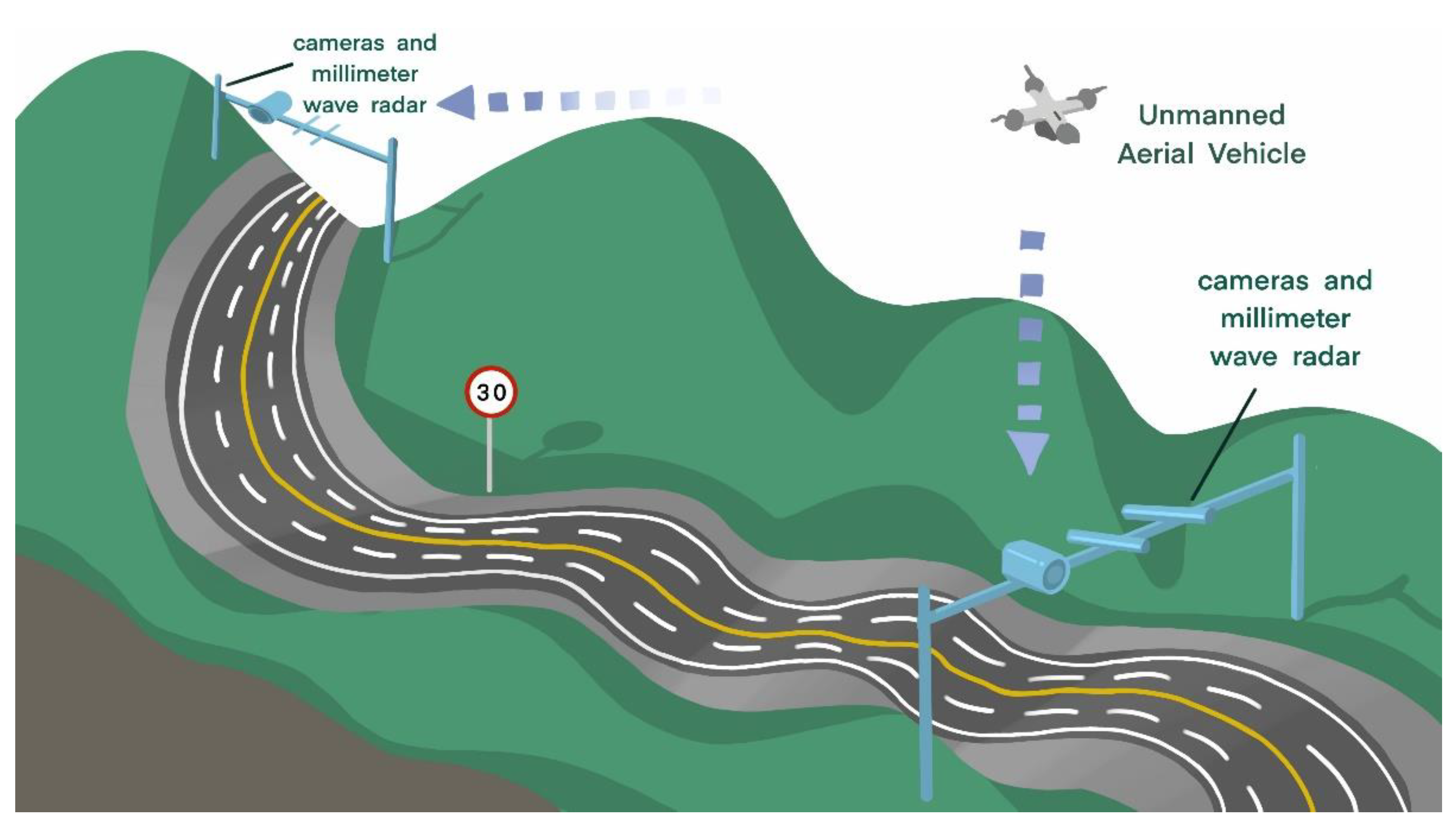
Traffic flow parameters such as traffic velocity and traffic density have a direct impact on the speed prediction of vehicles. As shown in Figure 8, traffic parameters are collected by roadside sensors (such as millimeter-wave radar, cameras, etc.) and high-altitude unmanned aerial vehicles. Accurate traffic historical data and real-time data are very important for the accurate prediction of traffic velocity. The data collected by the sensors is applied to macroscopic traffic flow models and learning models to predict traffic velocity in short and relatively long horizons.
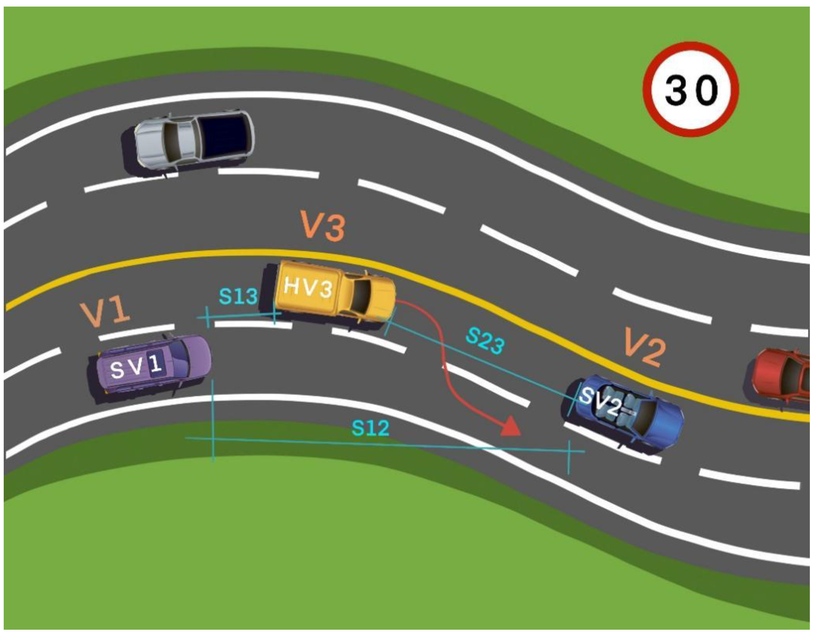
Once we understand the evolution of traffic flow and can predict changes in traffic parameters, we then need to understand the dynamics of the vehicles we are riding in. In order to improve traffic efficiency, we assume that the minimum speed of the vehicle is the traffic velocity at this time. However, to get to their destination earlier, passengers sometimes need to travel faster than the traffic speed. At this time, vehicle dynamics plays a key role in the decision-making and speed prediction of intelligent vehicles. Because at this time, whether in the curve or during an overtaking lane change condition, vehicle tire force is closer to its adhesion limit. As shown in Figure 9, when the host vehicle (HV3) is in these conditions, it needs to comprehensively consider the distance (s13 means the relative distance between HV3 and SV1, s23 means the relative distance between HV3 and SV2, s12 means the relative distance between SV1 and SV2), relative speed (V1, V2, V3 indicate the speed of the SV1, SV2, and HV3, respectively) with surrounding vehicles, and the speed limit on the curve. The vehicle needs to assess traffic risks and predict changes in its speed before performing these actions. At this time, the speed prediction is no longer passive, but an active planning process. Thus, one gets a more accurate prediction of speed when traffic flow and vehicle dynamics are taken into account.
For the problem of vehicle routing, most of the existing literature adopt the optimization of single objective as the criterion. This paper proposes a multi-objective optimization method for hybrid vehicle path planning as follows:

4.1. Vehicle Handling Stability Criterion Model by Neural Network

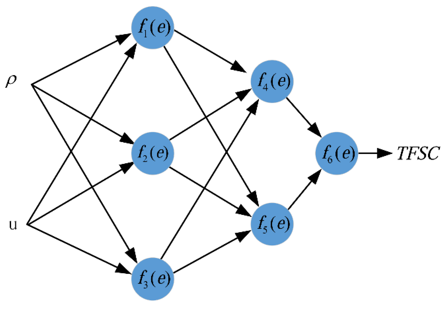
The vehicle handling stability criterion model is investigated with test data in this part. In this approach, previous measurements of traffic flow velocity and traffic density are mainly considered. An artificial neural network is represented in Figure 10. As the figure depicts, the inputs of the network include traffic flow speed and traffic density in Equation (1).
δ TFSC = f [ ρ ( 1 ) , ρ ( 2 ) , ρ ( 3 ) ρ ( n ) ; V ( ρ ( 1 ) ) , V ( ρ ( 2 ) ) , V ( ρ ( 3 ) ) V ( ρ ( n ) ) ] , .
where ρ ( 1 ) , ρ ( 2 ) , ρ ( 3 ) , …, ρ ( n ) are traffic density, V ( ρ ( 1 ) ) , V ( ρ ( 2 ) ) , V ( ρ ( 3 ) ) , …, V ( ρ ( n ) ) are traffic speed. The δ TFSC is the tire force saturation coefficient represented by Equations (2) and (3):
δ TFSCb = ( F xk μ F zk ) 2 + ( F yk F ymaxk ) 2 , .
δ TFSCmax = m a x ( ( F xk μ F zk ) 2 + ( F yk F ymaxk ) 2 ) , .
where: F xk , F yk , F zk are the longitudinal, lateral, and vertical tire forces of the vehicle tires, respectively; μ is the friction factor between the tire and the road; k is the number of the tire (specifically refers to four different tires); F ymaxk is the maximum lateral force of the k th tire.
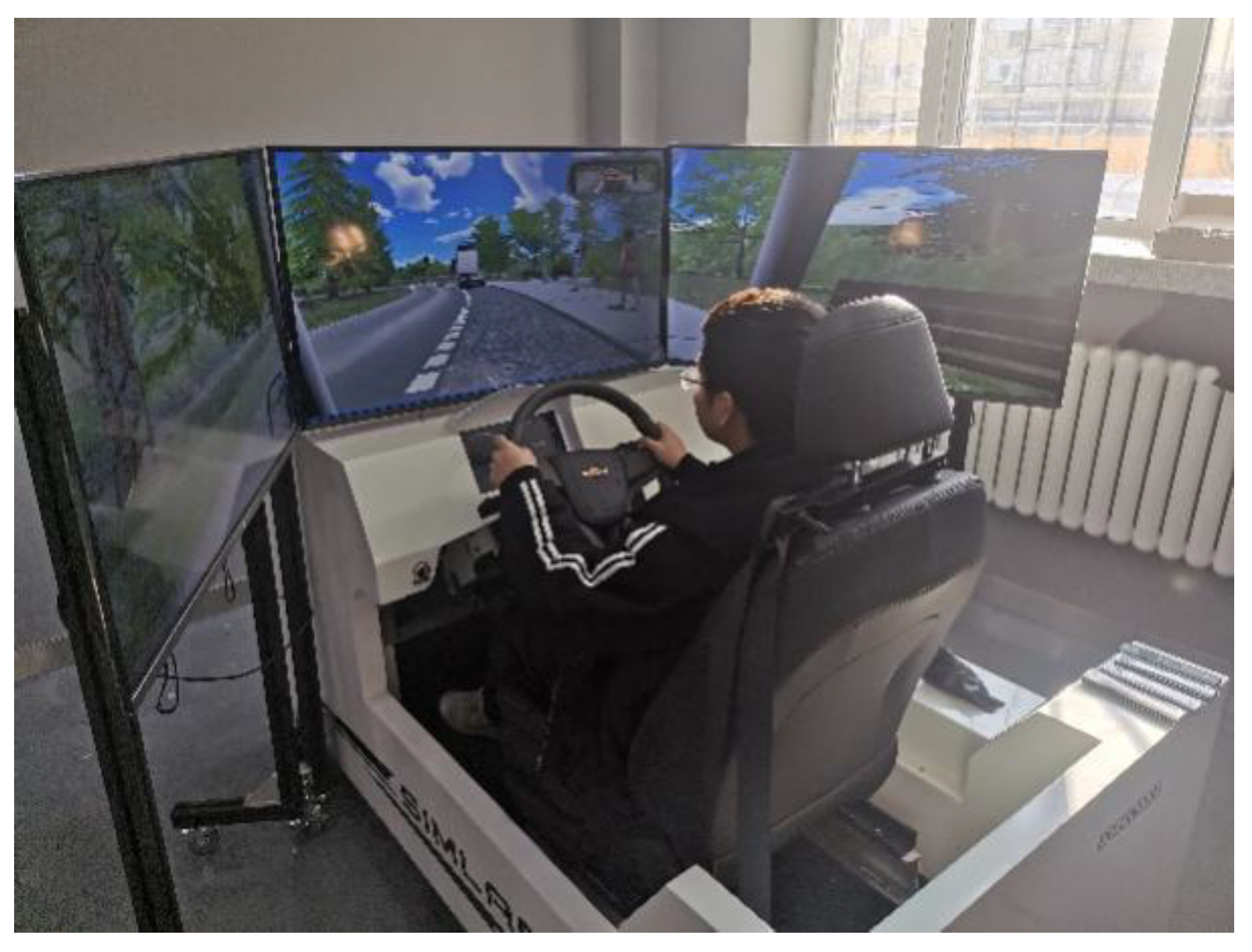
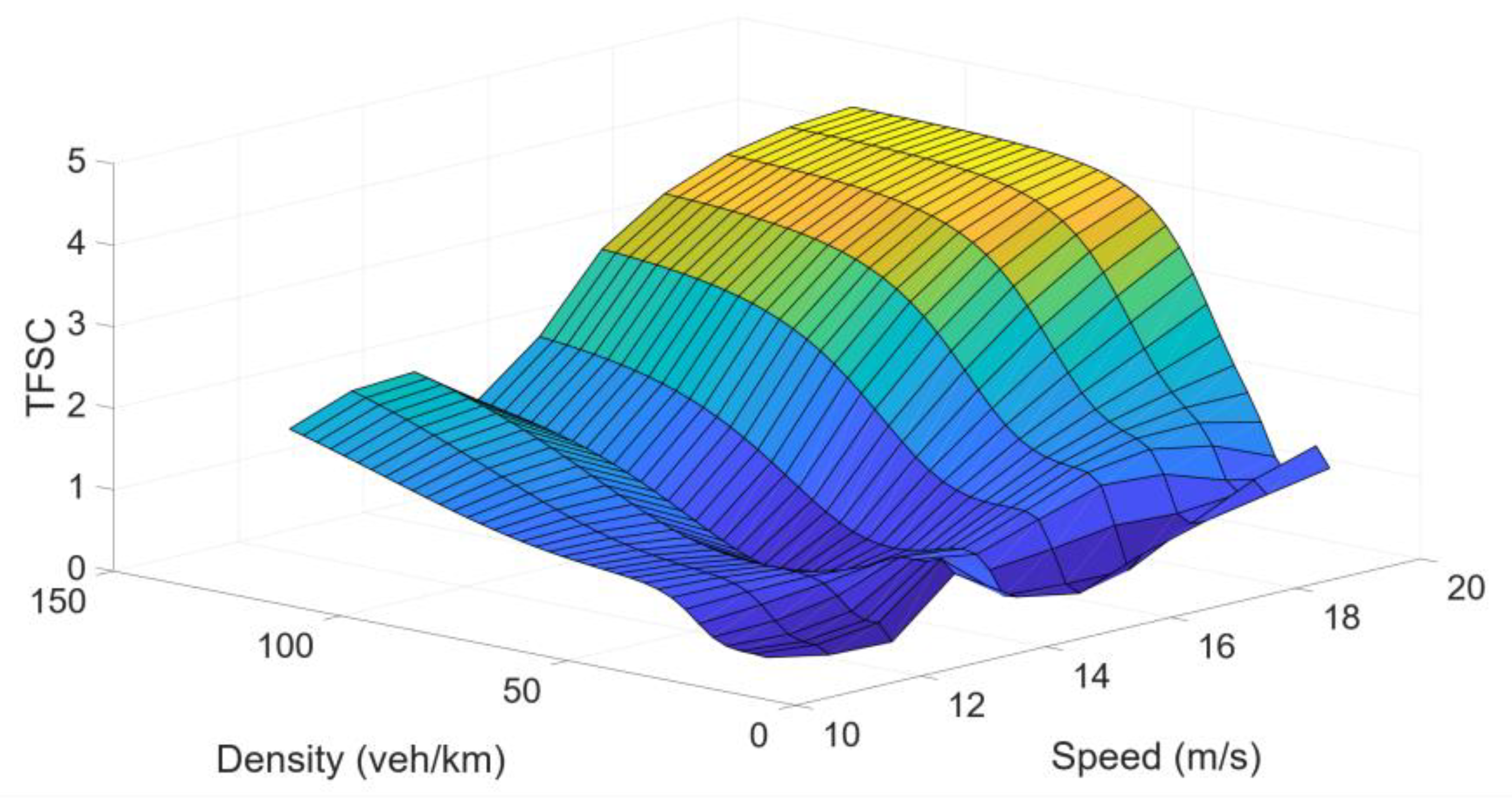
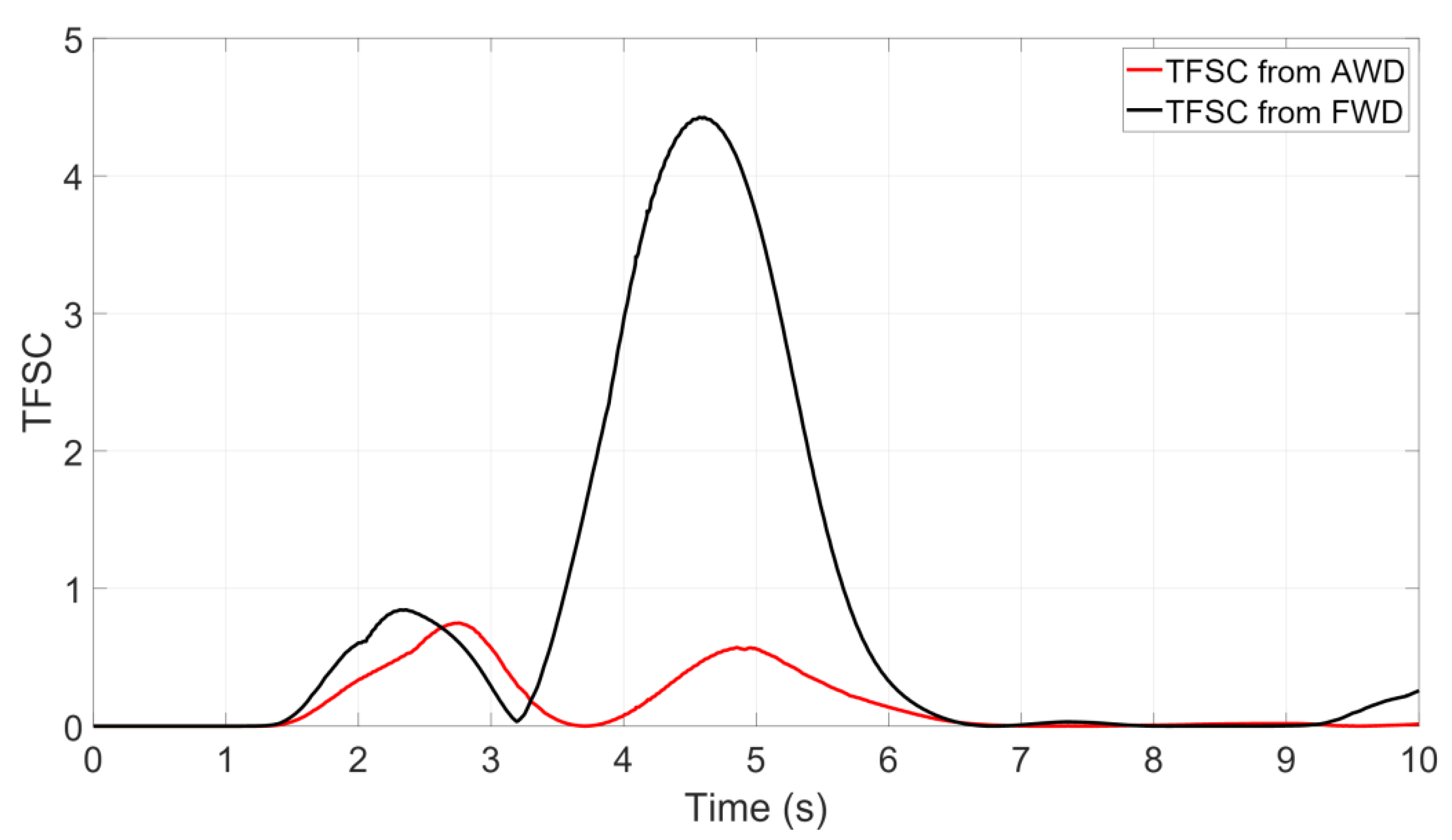
The idea of stability criteria model is that we first build the lateral dynamics model of the vehicle (please refer to our previous work [68]), and then we build the traffic environment shown in Figure 11. A driver-in-the-loop simulation environment for the presented scenario is shown in Figure 12. The traffic environment in the figure mainly shows two main traffic parameters: Distance and speed of SV and HV. Distance represents traffic density; at the same time, the speed of the SV indicates the speed of the traffic. We use this simulation environment to simulate the change in the saturation coefficient of the vehicle’s tires when the driver faces different traffic conditions and makes a lane change. For a front-wheel-drive ordinary vehicle, Figure 13 shows the change in the tire’s tire saturation coefficient as a function of traffic flow speed and density. As can be seen from Figure 13, the δ TFSC increases as the vehicle speed and density increase when the driver performs a lane change.

4.2. Multi-Objective Optimization Path Planning for Hybrid Vehicles

In this article, the speed prediction method based on the traffic flow model, speed prediction method based on traffic historical data and real-time data, and speed prediction method based on the vehicle lateral dynamics are reviewed. The relationship between the energy management method and speed prediction of HEVs is briefly summarized. The existing problems of speed prediction methods are presented and a new system structure of a hybrid electric vehicle is constructed. Based on the new system structure of the hybrid electric vehicle and the proposed stability criterion model, a vehicle path planning method and its application case based on the vehicle speed prediction method and vehicle lateral risk assessment are given below. According to the various traffic flow prediction methods reviewed above, this paper assumes that future traffic flow parameters, such as traffic density ρ and traffic velocity V, can be accurately predicted. Furthermore, the vehicle tire force saturation factor δ TFSC corresponding to each traffic density ρ and traffic velocity V was calculated by the vehicle stability criterion model established above. The constructed vehicle stability criterion model based on the use of tire force saturation factors can reflect the result of vehicle safety during driving. Next, the stability criterion model shown in Figure 13 will be used as the basis of the multi-objective optimization path planning to make the vehicle reach its destination safely, quickly, and efficiently. Driving safety, driving time, and energy consumption are trade-offs to achieve the best overall performance. The problem of vehicle path planning and selection is described as an optimization problem. The optimized performance indicators are described below.

4.2.1. Composite Index

The composite index { J com } is used to evaluate the overall performance of vehicle driving safety, time, and energy consumption, and the composite index is represented by Equation (4):
min J com = λ J s i + β J t i + γ J e i ,
where λ, β, γ represent the weighting factors of vehicle safety, travel time, and energy consumption, respectively.

4.2.2. Driving Safety Index

Using the steering stability criterion of the vehicle, the tire force saturation factor can be used to evaluate this basis, and the driving safety index can be represented by { J s i }. Driving safety is often the most important factor when the driver is driving a vehicle on the road. The larger the driving safety index { J s i }, the greater the influence of path security on the planning result.
J s i = e δ TFSC ( i ) ,

4.2.3. Travel Time Index

The driver expects that the driving time of the vehicle be as short as possible. However, most of the time, we have an expected period of time to arrive at our destination, and the weight function should reflect penalties that are greater than the expected time and rewards that are less than the expected time. The travel time index of the vehicle path can be represented by { J t i }:
J t i = { 0.8 + ( t i t lb ) t i < t lb 0.8 t lb t i t ub 0.8 + ( t i t ub ) t i > t ub ,
where { t i } is the travel time of the vehicle on the ith path, and t lb and t ub are the lower and upper bounds of the expected vehicle travel time, respectively.

4.2.4. Energy Expenditure Index

According to the longitudinal vehicle dynamics model, it can be seen that the vehicle is driving on a flat road, which means that there is no up and down gradient during the driving process [65]. At this time, the longitudinal dynamics model is expressed from Equations (7)–(10). The energy consumed is represented by Equation (11):
F ω = F air + F roll + F inertia ,
F air = C D A f 21.15 V 2 ,
F roll = m g f ,
F inertia = σ m d u d t ,
J e i = V t F ω ,
where C D is the coefficient of air resistance; A f is the front area of the vehicle; m is the vehicle quality; g is the acceleration of gravity; f is the rolling resistance coefficient; t is the time interval; σ is the rotating mass correction coefficient; F ω is the total resistance of the wheel when driving; F air is the air resistance; F roll is the rolling resistance; F inertia is the acceleration resistance; J e i is the energy consumed by the vehicle.

4.2.5. Determination of Weighting Factors

To compare the above three indexes, there is a need to weigh each of them by a coefficient. For driving safety index { J s i }, the weight factor {λ} is determined as follows (Equation (12)):
λ = { 1 , nomally η , other   characteristics ,
where η is adjusted according to the driver’s aggressiveness level, road friction coefficient, vehicle stability characteristics, etc. The travel time weighting factor β is determined as follows (Equation (13)):
β = { 1 , nomally κ , other   characteristics ,
where κ is determined according to the driver anxious degree, the congestion of the road network, rush hour, etc. Note that κ is used to avoid excessively congested roads.
Generally, we can find the shortest path from the starting point to the destination. Because the driver expects that the vehicle consumes as little energy as possible, we choose the energy consumed by the vehicle in the shortest route under a smooth traffic environment as a reference. The energy weight factor { γ } is determined as follows (Equation (14)):
γ = 1 J normal , .
where J normal is the normally expended energy or the average value of energy consumption from the beginning to the end.
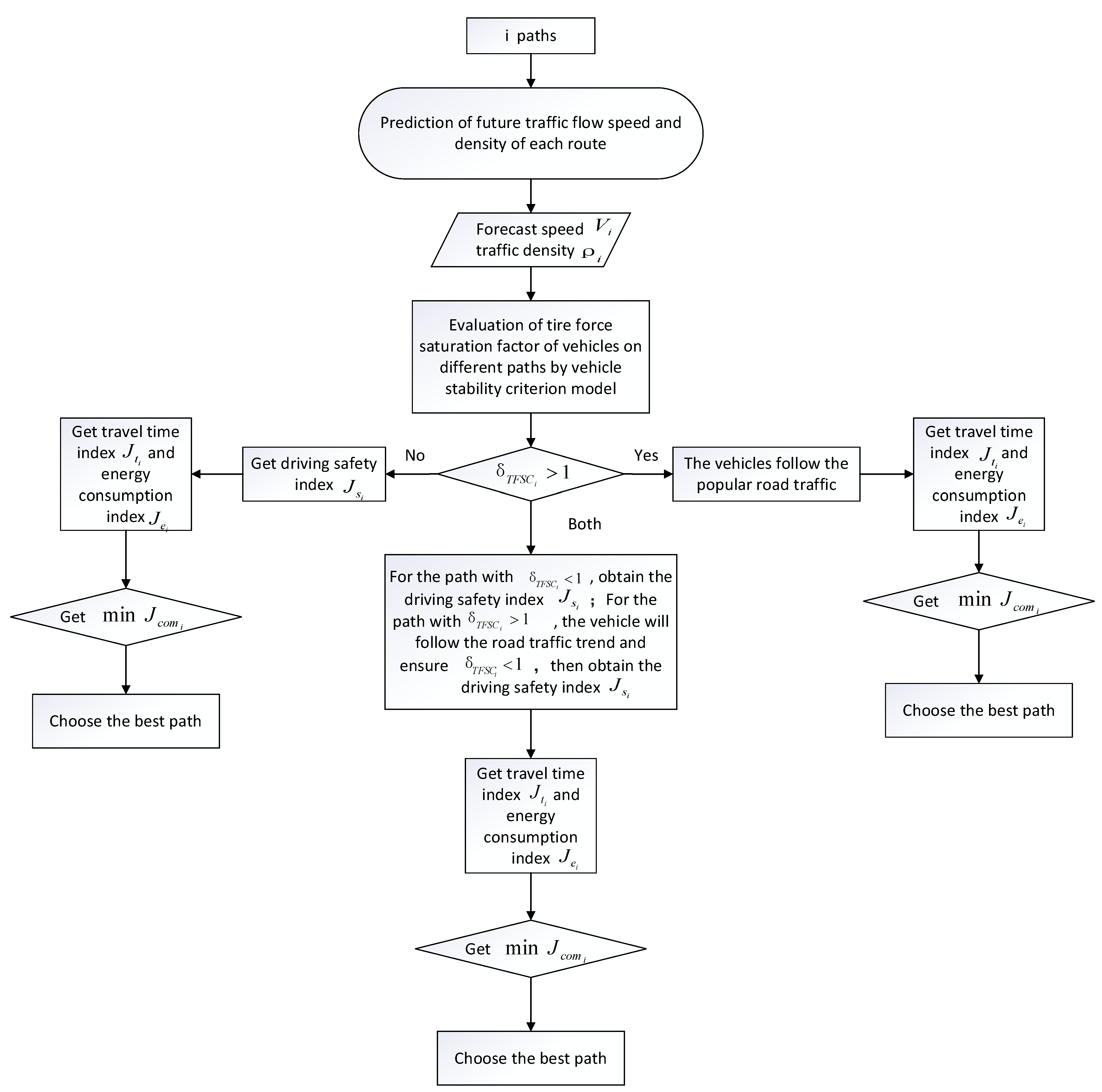
The control framework proposed in this section aims to find a trade-off between driving safety, driving time, and energy consumption during the vehicle driving process under the premise of ensuring the safety of the vehicle, so as to help the vehicle rationally plan and select the path. As shown in Figure 14, consider there are i paths available for vehicles to choose, and it is assumed that the parameters of traffic flow can be accurately predicted. Then, the vehicle stability criterion model is used to evaluate the stability of the future parameters of each path, and the saturation factor of the tire force δ TFSC is obtained when the vehicle is traveling at a predicted traffic density and speed in the future. To evaluate the tire force saturation factor of each path, if the tire force saturation factor of each path δ TFSC i < 1 , vehicles can adopt driving behavior strategies such as lateral overtaking and changing lanes, at this time, calculate the driving safety index of each path J s i . Then we calculate travel time index J t i and energy consumption index J e i of each path, respectively, by substituting the driving index of each path and the weighting factor corresponding to each index into the comprehensive index model to obtain the best path. If the tire force saturation factor of each path is δ TFSC i > 1 , drivers on such roads should avoid overtaking and changing lanes, and choose conservative driving behaviors, such as following the car in front. Under the premise of ensuring the safety of the vehicle, we then get the travel time index J t i and energy consumption index J e i of each path, and obtain the comprehensive index of each path and the weighting factor corresponding to each index. We then analyze the weight function “composite index” to get the best path. If some sections of a path have a criterion δ TFSC i < 1 and others sections have δ TFSC i > 1 , then it needs to be discussed separately. For the sections of δ TFSC i < 1 , vehicles are free to make overtaking lane changes. In the sections of δ TFSC i > 1 , in order to ensure the stability of the vehicle, the driver needs to follow the traffic flow instead of lane-changing and overtaking. At this time, we recalculate the driving safety index J s i , the travel time index J t i , and energy consumption index J e i of each path, and obtain the weighting factor corresponding to each index, using the composite index model to finally obtain the best choice path.

4.3. Path Planning Application

The process of achieving the path planning goals can be expressed as follows: The traffic parameter set P ( x , t ) (vehicle velocity, traffic density, etc.) is predicted for each sub-path, and it is provided to the vehicles in the traffic system so as to arrange the journey according to their respective characteristics. Then, through machine learning, the stability criterion model S ( ρ , u ) of all-wheel-drive (AWD) vehicles and front-wheel-drive (FWD) vehicles is established facing different traffic parameter sets P ( x , t ) . Then the optimal path is chosen according to S ( ρ , u ) . In the end, the optimal path for the current vehicle, among multiple paths, is obtained by using the multi-objective optimal path planning method J ( ρ , u ) proposed in this paper.
When the expected vehicle speed is higher than the traffic flow speed, it means that the vehicle needs to change lanes frequently. At a certain vehicle flow speed and density, the maximum front-wheel angle of a successful lane change can be predicted. Furthermore, we can calculate the lateral tire force of the vehicle through the vehicle lateral dynamics model. Similar to energy and time, the vehicle’s tire force saturation coefficient δ TFSC can be used as a basis for the vehicle’s path selection. Finally, depending on the travel time, energy consumption, environment (road friction coefficient), and vehicle characteristics (vehicle handling stability), one can choose a safe, efficient, and fast road for the driver.
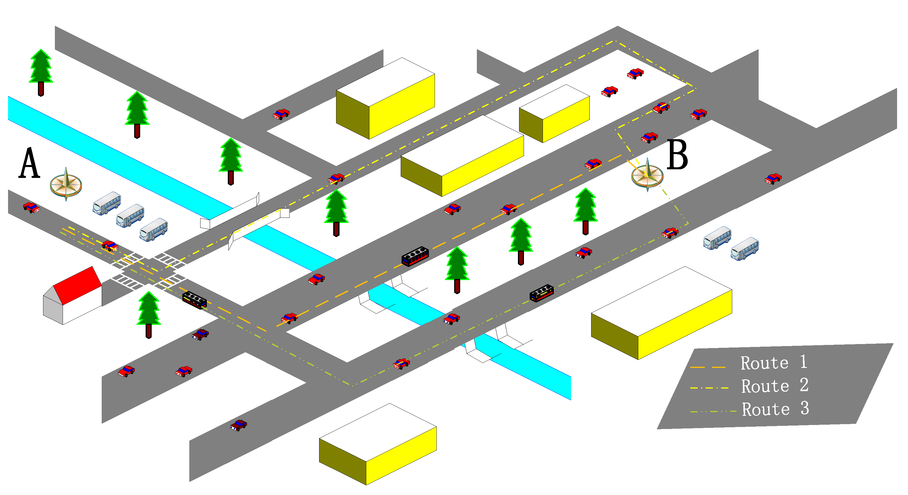
We consider route planning of a traffic system using traffic flow model and vehicle stability criterion as an example in Figure 15. Assume that Elbert intends to drive his vehicle from point A, seen on the left side of the figure, to point B, shown on the right side of the figure. There are three routes for Elbert to choose, namely Route 1, Route 2, and Route 3. Route 1 is closer, but the traffic flow is dense and the speed is slow. The distance of Route 2 is longer, but the traffic density is small and vehicle speed can be fast while traveling. The length and traffic flow of Route 3 are moderate, between Route 1 and Route 2, but road friction is poor. At this time, the predicted traffic flow parameters, the stability criterion model, and the multi-objective optimization route planning method can help Elbert select a safe, efficient, and fast road that matches the characteristics of his vehicle.
In addition, for the problem shown in Figure 15, we consider that Elbert encounters a rainy and snowy day (Route 1’s and Route 2’s tire-road friction coefficient is 0.4, Route 3’s friction coefficient is 0.1 due to road icing). According to the statement above, he will have different options to drive All-Wheel-Drive (AWD) and Front-Wheel-Drive (FWD) vehicles. Figure 11 shows a lane change and overtaking condition when the driver is close to the preceding vehicle, the target vehicle (HV)’s speed is large, and the front vehicle (SV)’s speed is small. Furthermore, Figure 16 shows the variation in δ TFSC for AWD and FWD vehicles at the same steering input in an overtaking and lane change condition from Route 1 [100]. We can observe that the FWD vehicle has been destabilized, but the AWD vehicle can keep the vehicle stable under such extreme conditions. For Route 3, where the road is icy, both AWD and FWD cannot stabilize the vehicle during a lane change and overtaking condition. Therefore, although the path 1 traffic flow speed is slow, when the driver drives the AWD vehicle, the destination can be reached faster by continuously overtaking and changing lanes. However, when driving a FWD vehicle, Path 2 would be a better choice.

5. Conclusions

Energy management strategies of new energy vehicles (NEVs) highly depend on accurate prediction of future velocity. In this paper, we present a review study on various vehicle speed prediction methods for NEVs. In this regard, various macroscopic traffic flow models, data-based traffic flow models, and the influence of vehicle lateral dynamics are introduced.
Through a detailed review and comparison of each method, it is clear that each approach is suitable for different application scenarios. Macroscopic and data-based traffic flow models are introduced and compared in terms of their pros and cons, potentially leading to better identification of development trends for prospective designers. Questions regarding the error in the macro traffic flow model, the magnitude of the error, and how to reduce the error with delay are to be answered. Moreover, prediction error between data-based and macro traffic models as well as how to combine these to reduce error remains an open headline.
Since the core issue of vehicle energy management is accurate speed forecast and planning, an emerging field, namely, vehicle stability control methods on speed prediction are investigated. Key questions on establishing a mixed traffic flow model and safety risk assessments are investigated from a traffic flow model and influence on vehicle lateral dynamics viewpoints.
The link between vehicle stability and energy efficiency is demonstrated by the application field of speed prediction methods. Benefitting from the fast development of vehicular technologies; software developers in the field of artificial intelligence; and sensors, cameras, and radars, potential future developments for velocity prediction methods could guide and inspire prospective researchers.
Lastly, examples of driving safety, traffic efficiency, and energy management are used to demonstrate the applications of speed prediction method based on vehicle handling dynamics and driving environment in path planning.

Funding

This research was funded by Northeast Forestry University No. 520-60201418.

Conflicts of Interest

The authors declare no conflict of interest.

References

  1. Li, K.Q.; Dai, Y.F.; Li, S.B.; Bian, M.Y. Development status and trend of intelligent connected vehicle (ICV) technology. J. Automot. Saf. Energy 2017, 8, 1–14. [Google Scholar]
  2. Pei, J.; Su, Y.; Zhang, D.; Qi, Y.; Leng, Z. Velocity forecasts using a combined deep learning model in hybrid electric vehicles with V2V and V2I communication. Sci. China Technol. Sci. 2020, 63, 55–64. [Google Scholar] [CrossRef]
  3. Hu, X.; Yuan, H.; Zou, C.; Li, Z.; Zhang, L. Co-estimation of state of charge and state of health for lithium-ion batteries based on fractional-order calculus. IEEE Trans. Veh. Technol. 2018, 67, 10319–10329. [Google Scholar] [CrossRef]
  4. Zhang, F.; Hu, X.; Langari, R.; Wang, L.; Cui, Y.; Pang, H. Adaptive energy management in automated hybrid electric vehicles with flexible torque request. Energy 2021, 214, 118873. [Google Scholar] [CrossRef]
  5. Zhang, F.; Hu, X.; Liu, T.; Duan, Z.; Xu, K.; Pang, H. Computationally Efficient Energy Management for Hybrid Electric Vehicles Using Model Predictive Control and Vehicle-to-Vehicle Communication. IEEE Trans. Veh. Technol. 2020, 70, 237–250. [Google Scholar] [CrossRef]
  6. Hu, X.; Zou, C.; Tang, X.; Liu, T.; Hu, L. Cost-optimal energy management of hybrid electric vehicles using fuel cell/battery health-aware predictive control. IEEE Trans. Power Electron. 2019, 35, 382–392. [Google Scholar] [CrossRef] [Green Version]
  7. Yang, S.; Wang, J.; Zhang, F.; Xi, J. Self-adaptive Equivalent Consumption Minimization Strategy for Hybrid Electric Vehicles. IEEE Trans. Veh. Technol. 2020, 70, 189–202. [Google Scholar] [CrossRef]
  8. China Association of Automobile Manufacturers. 2021. Available online: http://en.caam.org.cn/ (accessed on 1 June 2021).
  9. Taha, A.E.; AbuAli, N. Route planning considerations for autonomous vehicles. IEEE Commun. Mag. 2018, 56, 78–84. [Google Scholar] [CrossRef]
  10. Lu, J.; Cheng, Z.Y. Research progress in road traffic network security risk identification. J. Southeast Univ. 2019, 49. [Google Scholar]
  11. Huang, H.L.; Jiang, M.X.; Han, C.Y.; Xu, G.M. Multi-class user traffic assignment model based on safety and reliability. China J. Highw. Transp. 2018, 31, 312–321. [Google Scholar]
  12. Zhang, F.; Wang, L.; Coskun, S.; Pang, H.; Cui, Y.; Xi, J. Energy management strategies for hybrid electric vehicles: Review, classification, comparison, and outlook. Energies 2020, 13, 3352. [Google Scholar] [CrossRef]
  13. Zhang, F.; Hu, X.; Langari, R.; Cao, D. Energy management strategies of connected HEVs and PHEVs: Recent progress and outlook. Prog. Energy Combust. Sci. 2019, 73, 235–256. [Google Scholar] [CrossRef]
  14. Tran, D.D.; Vafaeipour, M.; El Baghdadi, M.; Barrero, R.; Van Mierlo, J.; Hegazy, O. Thorough state-of-the-art analysis of electric and hybrid vehicle powertrains: Topologies and integrated energy management strategies. Renew. Sustain. Energy Rev. 2020, 119, 109596. [Google Scholar] [CrossRef]
  15. Zhou, Y.; Ravey, A.; Péra, M.C. A survey on driving prediction techniques for predictive energy management of plug-in hybrid electric vehicles. J. Power Sources 2019, 412, 480–495. [Google Scholar] [CrossRef] [Green Version]
  16. Djahel, S.; Doolan, R.; Muntean, G.M.; Murphy, J. A communications-oriented perspective on traffic management systems for smart cities: Challenges and innovative approaches. IEEE Commun. Surv. Tutor. 2014, 17, 125–151. [Google Scholar] [CrossRef]
  17. Papamichail, I.; Bekiaris-Liberis, N.; Delis, A.I.; Manolis, D.; Mountakis, K.S.; Nikolos, I.K.; Papageorgiou, M. Motorway traffic flow modelling, estimation and control with vehicle automation and communication systems. Annu. Rev. Control 2019, 48, 325–346. [Google Scholar] [CrossRef]
  18. Seo, T.; Bayen, A.M.; Kusakabe, T.; Asakura, Y. Traffic state estimation on highway: A comprehensive survey. Annu. Rev. Control 2017, 43, 128–151. [Google Scholar] [CrossRef] [Green Version]
  19. Van Wageningen-Kessels, F.; Van Lint, H.; Vuik, K.; Hoogendoorn, S. Genealogy of traffic flow models. EURO J. Transp. Logist. 2015, 4, 445–473. [Google Scholar] [CrossRef] [Green Version]
  20. Hoogendoorn, S.P.; Bovy, P.H. State-of-the-art of vehicular traffic flow modelling. Proc. Inst. Mech. Eng. Part I J. Syst. Control Eng. 2001, 215, 283–303. [Google Scholar] [CrossRef]
  21. Lighthill, M.J.; Whitham, G.B. On kinematic waves II. A theory of traffic flow on long crowded roads. Proc. R. Soc. London. Ser. A Math. Phys. Sci. 1955, 229, 317–345. [Google Scholar]
  22. Jin, W.L.; Zhang, H.M. The formation and structure of vehicle clusters in the Payne–Whitham traffic flow model. Transp. Res. Part B Methodol. 2003, 37, 207–223. [Google Scholar] [CrossRef]
  23. Papageorgiou, M.; Blosseville, J.M.; Hadj-Salem, H. Macroscopic modelling of traffic flow on the Boulevard Périphérique in Paris. Transp. Res. Part B Methodol. 1989, 23, 29–47. [Google Scholar] [CrossRef]
  24. Zhang, H.M. A non-equilibrium traffic model devoid of gas-like behavior. Transp. Res. Part B Methodol. 2002, 36, 275–290. [Google Scholar] [CrossRef]
  25. Lebacque, J.P.; Mammar, S.; Haj-Salem, H. The Aw–Rascle and Zhang’s model: Vacuum problems, existence and regularity of the solutions of the Riemann problem. Transp. Res. Part B Methodol. 2007, 41, 710–721. [Google Scholar] [CrossRef]
  26. Blandin, S.; Work, D.; Goatin, P.; Piccoli, B.; Bayen, A. A general phase transition model for vehicular traffic. SIAM J. Appl. Math. 2011, 71, 107–127. [Google Scholar] [CrossRef] [Green Version]
  27. Delis, A.I.; Nikolos, I.K.; Papageorgiou, M. High-resolution numerical relaxation approximations to second-order macroscopic traffic flow models. Transp. Res. Part C Emerg. Technol. 2014, 44, 318–349. [Google Scholar] [CrossRef]
  28. Crandall, M.G.; Ishii, H.; Lions, P.L. User’s guide to viscosity solutions of second order partial differential equations. Bull. Am. Math. Soc. 1992, 27, 1–67. [Google Scholar] [CrossRef] [Green Version]
  29. Claudel, C.G.; Bayen, A.M. Lax–Hopf based incorporation of internal boundary conditions into Hamilton–Jacobi equation. Part I: Theory. IEEE Trans. Autom. Control 2010, 55, 1142–1157. [Google Scholar] [CrossRef]
  30. Laval, J.A.; Leclercq, L. The Hamilton–Jacobi partial differential equation and the three representations of traffic flow. Transp. Res. Part B Methodol. 2013, 52, 17–30. [Google Scholar] [CrossRef]
  31. Jin, W.L. On the equivalence between continuum and car-following models of traffic flow. Transp. Res. Part B Methodol. 2016, 93, 543–559. [Google Scholar] [CrossRef] [Green Version]
  32. Madaan, N.; Sharma, S. A lattice model accounting for multi-lane traffic system. Phys. A Stat. Mech. Appl. 2021, 564, 125446. [Google Scholar] [CrossRef]
  33. Costeseque, G.; Duret, A. Mesoscopic multiclass traffic flow modeling on multi-lane sections. In Proceedings of the 95th Annual Meeting Trans-portation Research Board-TRB, Transportation Research Board, Washington, DC, USA, 10–14 January 2016; p. 27. [Google Scholar]
  34. Sumalee, A.; Zhong, R.X.; Pan, T.L.; Szeto, W.Y. Stochastic cell transmission model (SCTM): A stochastic dynamic traffic model for traffic state surveillance and assignment. Transp. Res. Part B Methodol. 2011, 45, 507–533. [Google Scholar] [CrossRef]
  35. Jabari, S.E.; Zheng, J.; Liu, H.X. A probabilistic stationary speed–density relation based on Newell’s simplified car-following model. Transp. Res. Part B Methodol. 2014, 68, 205–223. [Google Scholar] [CrossRef]
  36. Jabari, S.E.; Liu, H.X. A stochastic model of traffic flow: Theoretical foundations. Transp. Res. Part B Methodol. 2012, 46, 156–174. [Google Scholar] [CrossRef]
  37. Wada, K.; Usui, K.; Takigawa, T.; Kuwahara, M. An optimization modeling of coordinated traffic signal control based on the variational theory and its stochastic extension. Transp. Res. Proedria 2017, 23, 624–644. [Google Scholar] [CrossRef]
  38. Liu, Z.; Liu, Y.; Meng, Q.; Cheng, Q. A tailored machine learning approach for urban transport network flow estimation. Transp. Res. Part C Emerg. Technol. 2019, 108, 130–150. [Google Scholar] [CrossRef]
  39. Mackenzie, J.; Roddick, J.F.; Zito, R. An evaluation of HTM and LSTM for short-term arterial traffic flow prediction. IEEE Trans. Intell. Transp. Syst. 2018, 20, 1847–1857. [Google Scholar] [CrossRef]
  40. Zhu, L.; Yu, F.R.; Wang, Y.; Ning, B.; Tang, T. Big data analytics in intelligent transportation systems: A survey. IEEE Trans. Intell. Transp. Syst. 2018, 20, 383–398. [Google Scholar] [CrossRef]
  41. Malek, Y.N.; Najib, M.; Bakhouya, M.; Essaaidi, M. Multivariate deep learning approach for electric vehicle speed forecasting. Big Data Min. Anal. 2020, 4, 56–64. [Google Scholar] [CrossRef]
  42. Lin, X.; Wang, Z.; Wu, J. Energy management strategy based on velocity prediction using back propagation neural network for a plug-in fuel cell electric vehicle. Int. J. Energy Res. 2021, 45, 2629–2643. [Google Scholar] [CrossRef]
  43. Nallaperuma, D.; Nawaratne, R.; Bandaragoda, T.; Adikari, A.; Nguyen, S.; Kempitiya, T.; Pothuhera, D. Online incremental machine learning platform for big data-driven smart traffic management. IEEE Trans. Intell. Transp. Syst. 2019, 20, 4679–4690. [Google Scholar] [CrossRef]
  44. Kong, F.; Li, J.; Jiang, B.; Song, H. Short-term traffic flow prediction in smart multimedia system for Internet of Vehicles based on deep belief network. Future Gener. Comput. Syst. 2019, 93, 460–472. [Google Scholar] [CrossRef]
  45. Zang, D.; Ling, J.; Wei, Z.; Tang, K.; Cheng, J. Long-term traffic speed prediction based on multiscale spatio-temporal feature learning network. IEEE Trans. Intell. Transp. Syst. 2018, 20, 3700–3709. [Google Scholar] [CrossRef]
  46. Chen, M.; Yu, X.; Liu, Y. PCNN: Deep convolutional networks for short-term traffic congestion prediction. IEEE Trans. Intell. Transp. Syst. 2018, 19, 3550–3559. [Google Scholar] [CrossRef] [Green Version]
  47. Zhang, Y.; Cheng, T.; Ren, Y.; Xie, K. A novel residual graph convolution deep learning model for short-term network-based traffic forecasting. Int. J. Geogr. Inf. Sci. 2020, 34, 969–995. [Google Scholar] [CrossRef]
  48. Chen, W.; An, J.; Li, R.; Fu, L.; Xie, G.; Bhuiyan, M.Z.A.; Li, K. A novel fuzzy deep-learning approach to traffic flow prediction with uncertain spatial–temporal data features. Future Gener. Comput. Syst. 2018, 89, 78–88. [Google Scholar] [CrossRef]
  49. Tang, J.; Liu, F.; Zou, Y.; Zhang, W.; Wang, Y. An improved fuzzy neural network for traffic speed prediction considering periodic characteristic. IEEE Trans. Intell. Transp. Syst. 2017, 18, 2340–2350. [Google Scholar] [CrossRef]
  50. Qu, L.; Li, W.; Li, W.; Ma, D.; Wang, Y. Daily long-term traffic flow forecasting based on a deep neural network. Expert Syst. Appl. 2019, 121, 304–312. [Google Scholar] [CrossRef]
  51. Wu, Y.; Tan, H.; Qin, L.; Ran, B.; Jiang, Z. A hybrid deep learning based traffic flow prediction method and its understanding. Transp. Res. Part C Emerg. Technol. 2018, 90, 166–180. [Google Scholar] [CrossRef]
  52. Han, L.; Huang, Y.S. Short-term traffic flow prediction of road network based on deep learning. IET Intell. Transp. Syst. 2020, 14, 495–503. [Google Scholar] [CrossRef]
  53. Li, L.; Qin, L.; Qu, X.; Zhang, J.; Wang, Y.; Ran, B. Day-ahead traffic flow forecasting based on a deep belief network optimized by the multi-objective particle swarm algorithm. Knowl. Based Syst. 2019, 172, 1–14. [Google Scholar] [CrossRef]
  54. Shin, J.; Yeon, K.; Kim, S.; Sunwoo, M.; Han, M. Comparative Study of Markov Chain with Recurrent Neural Network for Short Term Velocity Prediction Implemented on an Embedded System. IEEE Access 2021, 9, 24755–24767. [Google Scholar] [CrossRef]
  55. Guo, Y.; Li, Z.; Liu, P.; Wu, Y. Modeling correlation and heterogeneity in crash rates by collision types using full Bayesian random parameters multivariate Tobit model. Accid. Anal. Prev. 2019, 128, 164–174. [Google Scholar] [CrossRef] [PubMed]
  56. Rahman, M.S.; Abdel-Aty, M. Longitudinal safety evaluation of connected vehicles’ platooning on expressways. Accid. Anal. Prev. 2018, 117, 381–391. [Google Scholar] [CrossRef]
  57. Wen-Xing, Z.; Li-Dong, Z. A new car-following model for autonomous vehicles flow with mean expected velocity field. Phys. A Stat. Mech. Its Appl. 2018, 492, 2154–2165. [Google Scholar] [CrossRef]
  58. Zhu, W.X.; Zhang, H.M. Analysis of mixed traffic flow with human-driving and autonomous cars based on car-following model. Phys. A Stat. Mech. Appl. 2018, 496, 274–285. [Google Scholar] [CrossRef]
  59. Li, G.; Yang, Y.; Zhang, T.; Qu, X.; Cao, D.; Cheng, B.; Li, K. Risk assessment based collision avoidance decision-making for autonomous vehicles in multi-scenarios. Transp. Res. Part C Emerg. Technol. 2021, 122, 102820. [Google Scholar] [CrossRef]
  60. Zhang, L.; Wang, S.; Chen, C.; Yang, M.; Zhe, X. Lane-changing risk model for expressway exit zone based on natural driving data. J. Tongji Univ. 2019, 47, 1446–1453. [Google Scholar]
  61. Peng, Z.; Gao, S.; Li, Z.; Xiao, B.; Qian, Y. Vehicle safety improvement through deep learning and mobile sensing. IEEE Netw. 2018, 32, 28–33. [Google Scholar] [CrossRef]
  62. Yu, Z.; Feng, Y.; Xiong, L. Review on vehicle dynamics control of distributed drive electric vehicle. Jixie Gongcheng Xuebao (Chin. J. Mech. Eng.) 2013, 49, 105–114. [Google Scholar] [CrossRef]
  63. Jiang, K.; Yang, D.; Xie, S.; Xiao, Z.; Victorino, A.; Charara, A. Real-time estimation and prediction of tire forces using digital map for driving risk assessment. Transp. Res. Part C Emerg. Technol. 2019, 107, 463–489. [Google Scholar] [CrossRef]
  64. Lin, Y.; Nguyen, H.; Balas, V.; Lin, T.; Kuo, I. Adaptive prediction-based control for an ecological cruise control system on curved and hilly roads. J. Intell. Fuzzy Syst. 2020, 38, 6129–6144. [Google Scholar] [CrossRef]
  65. Chu, D.; Li, Z.; Wang, J.; Wu, C.; Hu, Z. Rollover speed prediction on curves for heavy vehicles using mobile smartphone. Measurement 2018, 130, 404–411. [Google Scholar] [CrossRef]
  66. Imine, H.; Benallegue, A.; Madani, T.; Srairi, S. Rollover Risk Prediction of Heavy Vehicle Using High-Order Sliding-Mode Observer: Experimental Results. IEEE Trans. Veh. Technol. 2014, 63, 2533–2543. [Google Scholar] [CrossRef]
  67. Liu, K.; Gong, J.; Chen, S.; Zhang, Y.; Chen, H. Model Predictive Stabilization Control of High-Speed Autonomous Ground Vehicles Considering the Effect of Road Topography. Appl. Sci. 2018, 8, 822. [Google Scholar] [CrossRef] [Green Version]
  68. Li, L.; Coskun, S.; Zhang, F.; Langari, R.; Xi, J. Energy Management of Hybrid Electric Vehicle Using Vehicle Lateral Dynamic in Velocity Prediction. IEEE Trans. Veh. Technol. 2019, 68, 3279–3293. [Google Scholar] [CrossRef]
  69. Song, P.; Gao, B.; Xie, S.; Fang, R. Optimal Predictive Control for Path Following of a Full Drive-by-Wire Vehicle at Varying Speeds. Chin. J. Mech. Eng. 2017, 30, 711–721. [Google Scholar] [CrossRef]
  70. Krid, M.; Benamar, F.; Zamzami, Z. Design of an active device for controlling lateral stability of fast mobile robot. Robotica 2016, 34, 2629–2651. [Google Scholar] [CrossRef]
  71. Ren, H.; Chen, S.; Yang, L.; Zhao, Y. Optimal Path Planning and Speed Control Integration Strategy for UGVs in Static and Dynamic Environments. IEEE Trans. Veh. Technol. 2020, 69, 10619–10629. [Google Scholar] [CrossRef]
  72. Jin, X.J.; Yin, G.; Chen, N. Gain-scheduled robust control for lateral stability of four-wheel-independent-drive electric vehicles via linear parameter-varying technique. Mechatronics 2015, 30, 286–296. [Google Scholar] [CrossRef]
  73. Coskun, S.; Li, L. Vehicle lateral motion control via robust delay-dependent Takagi-Sugeno strategy. Trans. Inst. Meas. Control 2021, 43, 1430–1444. [Google Scholar] [CrossRef]
  74. Coskun, S. Autonomous overtaking in highways: A receding horizon trajectory generator with embedded safety feature. Eng. Sci. Technol. Int. J. 2021. [Google Scholar] [CrossRef]
  75. Wang, R.; Hu, C.; Yan, F.; Chadli, M. Composite nonlinear feedback control for path following of four-wheel independently actuated autonomous ground vehicles. IEEE Trans. Intell. Transp. Syst. 2016, 17, 2063–2074. [Google Scholar] [CrossRef]
  76. Guo, J.; Luo, Y.; Li, K. Dynamic coordinated control for over-actuated autonomous electric vehicles with nonholonomic constraints via nonsingular terminal sliding mode technique. Nonlinear Dyn. 2016, 85, 583–597. [Google Scholar] [CrossRef]
  77. Abzi, I.; Kabbaj, M.N.; Benbrahim, M. Fault tolerant control of vehicle lateral dynamic using a new pneumatic forces multiple model. Actuators 2020, 9, 120. [Google Scholar] [CrossRef]
  78. Yang, X.; Wang, Z.; Peng, W. Coordinated control of AFS and DYC for vehicle handling and stability based on optimal guaranteed cost theory. Veh. Syst. Dyn. 2009, 47, 57–79. [Google Scholar] [CrossRef]
  79. Zhang, H.; Zhang, X.; Wang, J. Robust gain-scheduling energy-to-peak control of vehicle lateral dynamics stabilisation. Veh. Syst. Dyn. 2014, 52, 309–340. [Google Scholar] [CrossRef]
  80. Zhang, H.; Wang, J. Vehicle lateral dynamics control through AFS/DYC and robust gain-scheduling approach. IEEE Trans. Veh. Technol. 2015, 65, 489–494. [Google Scholar] [CrossRef]
  81. Li, B.; Goodarzi, A.; Khajepour, A.; Chen, S.K.; Litkouhi, B. An optimal torque distribution control strategy for four-independent wheel drive electric vehicles. Veh. Syst. Dyn. 2015, 53, 1172–1189. [Google Scholar] [CrossRef]
  82. Yang, W.; Zheng, L.; Li, Y.; Ren, Y.; Xiong, Z. Automated highway driving decision considering driver characteristics. IEEE Trans. Intell. Transp. Syst. 2019, 21, 2350–2359. [Google Scholar] [CrossRef]
  83. Conti, J.; Holtberg, P.; Diefenderfer, J.; LaRose, A.; Turnure, J.T.; Westfall, L. International Energy Outlook 2016 with Projections to 2040; No. DOE/EIA-0484 (2016); Office of Energy Analysis, USDOE Energy Information Administration (EIA): Washington, DC, USA, 2016.
  84. Ramachandran, S.; Stimming, U. Well to wheel analysis of low carbon alternatives for road traffic. Energy Environ. Sci. 2015, 8, 3313–3324. [Google Scholar] [CrossRef] [Green Version]
  85. Huang, Y.; Wang, H.; Khajepour, A.; Li, B.; Ji, J.; Zhao, K.; Hu, C. A review of power management strategies and component sizing methods for hybrid vehicles. Renew. Sustain. Energy Rev. 2018, 96, 132–144. [Google Scholar] [CrossRef]
  86. Li, J.; Zhou, Q.; He, Y.; Shuai, B.; Li, Z.; Williams, H.; Xu, H. Dual-loop online intelligent programming for driver-oriented predict energy management of plug-in hybrid electric vehicles. Appl. Energy 2019, 253, 113617. [Google Scholar] [CrossRef] [Green Version]
  87. Zhou, Y.; Li, H.; Ravey, A.; Péra, M.C. An integrated predictive energy management for light-duty range-extended plug-in fuel cell electric vehicle. J. Power Sources 2020, 451, 227780. [Google Scholar] [CrossRef]
  88. Jinquan, G.; Hongwen, H.; Jiankun, P.; Nana, Z. A novel MPC-based adaptive energy management strategy in plug-in hybrid electric vehicles. Energy 2019, 175, 378–392. [Google Scholar] [CrossRef]
  89. Li, G.; Görges, D. Energy management strategy for parallel hybrid electric vehicles based on approximate dynamic programming and velocity forecast. J. Frankl. Inst. 2019, 356, 9502–9523. [Google Scholar] [CrossRef]
  90. Guo, J.; He, H.; Sun, C. ARIMA-based road gradient and vehicle velocity prediction for hybrid electric vehicle energy management. IEEE Trans. Veh. Technol. 2019, 68, 5309–5320. [Google Scholar] [CrossRef]
  91. Chen, Z.; Hu, H.; Wu, Y.; Zhang, Y.; Li, G.; Liu, Y. Stochastic model predictive control for energy management of power-split plug-in hybrid electric vehicles based on reinforcement learning. Energy 2020, 211, 118931. [Google Scholar] [CrossRef]
  92. Lian, R.; Tan, H.; Peng, J.; Li, Q.; Wu, Y. Cross-type transfer for deep reinforcement learning based hybrid electric vehicle energy management. IEEE Trans. Veh. Technol. 2020, 69, 8367–8380. [Google Scholar] [CrossRef]
  93. Zhai, C.; Luo, F.; Liu, Y. A novel predictive energy management strategy for electric vehicles based on velocity prediction. IEEE Trans. Veh. Technol. 2020, 69, 12559–12569. [Google Scholar] [CrossRef]
  94. Chen, H.; Guo, L.; Ding, H.; Li, Y.; Gao, B. Real-time predictive cruise control for eco-driving taking into account traffic constraints. IEEE Trans. Intell. Transp. Syst. 2018, 20, 2858–2868. [Google Scholar] [CrossRef]
  95. Xie, S.; Qi, S.; Lang, K.; Tang, X.; Lin, X. Coordinated management of connected plug-in hybrid electric buses for energy saving, inter-vehicle safety, and battery health. Appl. Energy 2020, 268, 115028. [Google Scholar] [CrossRef]
  96. Li, Y.; Zhang, J.; Lv, C.; Yuan, Y. Coordinated control of the steering system and the distributed motors for comprehensive optimization of the dynamics performance and the energy consumption of an electric vehicle. Proc. Inst. Mech. Eng. Part D J. Automob. Eng. 2017, 231, 1605–1626. [Google Scholar] [CrossRef]
  97. Ahmed, A.A.; Ramadan, H.S. Prototype implementation of advanced electric vehicles drivetrain system: Verification and validation. Appl. Energy 2020, 266, 114807. [Google Scholar] [CrossRef]
  98. Guo, L.; Gao, B.; Gao, Y.; Chen, H. Optimal energy management for HEVs in eco-driving applications using bi-level MPC. IEEE Trans. Intell. Transp. Syst. 2016, 18, 2153–2162. [Google Scholar] [CrossRef]
  99. Alcantar, J.V.; Assadian, F. Vehicle dynamics control of an electric-all-wheel-drive hybrid electric vehicle using tyre force optimization and allocation. Veh. Syst. Dyn. 2019, 57, 1897–1923. [Google Scholar] [CrossRef]
  100. Li, L.; Pei, Y.; Yin, L.; Zhou, L. Vehicle Path Planning Based on Stability and Macroscopic Traffic Flow Model. China J. Highw. Transp. 2020, 33, 71–80. [Google Scholar]
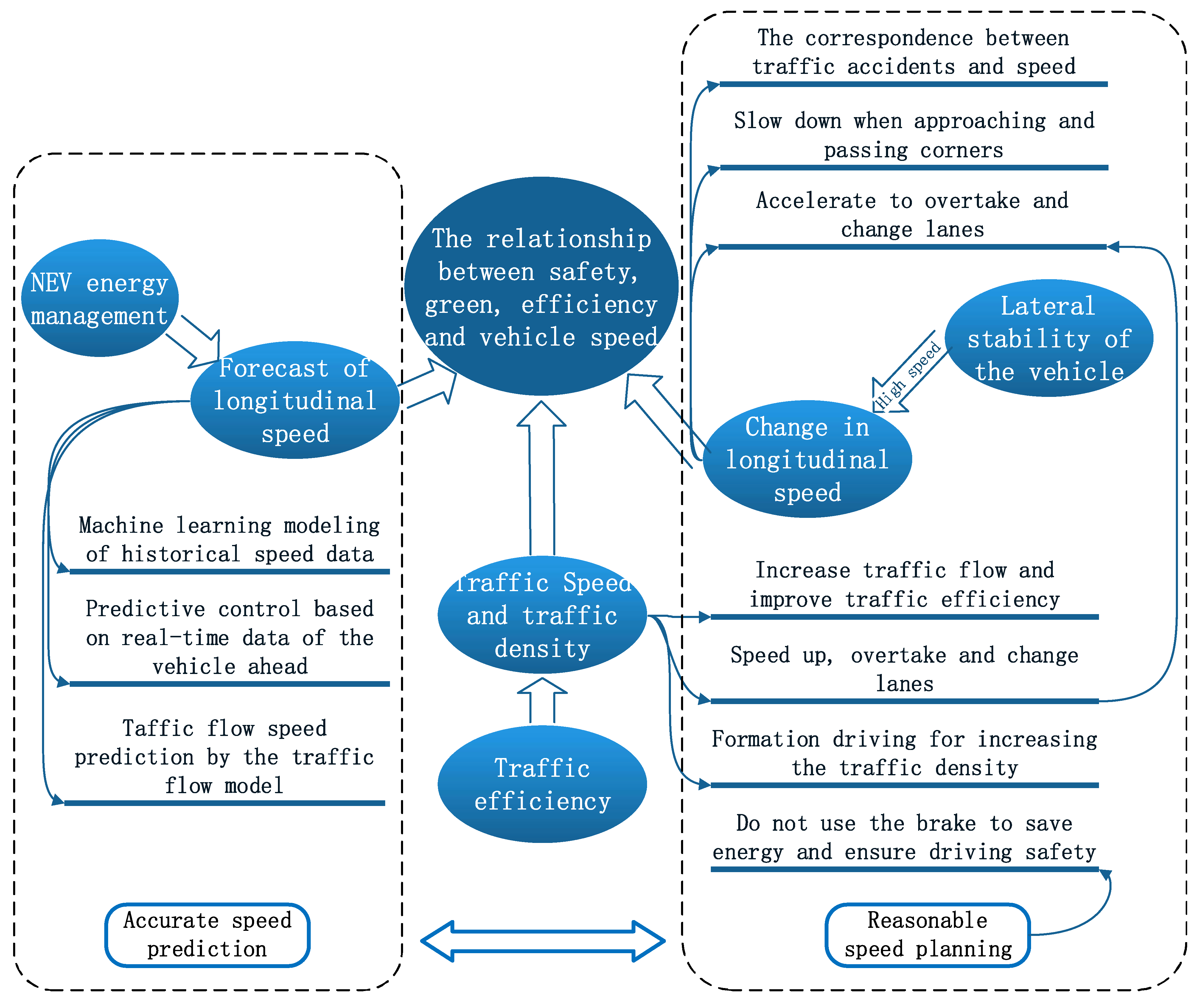
Figure 1. The relationship between “safety”, “efficiency”, “green”, and speed of intelligent networked vehicles.
Energies 14 03431 g001
Figure 2. Comparison of production and sales volume of new energy vehicles in China in recent three years.
Energies 14 03431 g002
Figure 3. Research framework of road traffic network security risk identification.
Energies 14 03431 g003
Figure 4. Online classification of energy management algorithms.
Energies 14 03431 g004
Figure 5. Power system layout structure of a four-wheel independent control electric vehicle.
Energies 14 03431 g005
Figure 6. The layout structure of the power system of an ordinary front-wheel steering HEV bus.
Energies 14 03431 g006
Figure 7. The layout structure of the power system of an all-wheel-steer distributed-drive new energy vehicle.
Energies 14 03431 g007
Figure 8. Use traffic sensors to collect changes in traffic parameters.
Energies 14 03431 g008
Figure 9. An example of the influence of vehicle lateral dynamics on lane change decisions and speed prediction.
Energies 14 03431 g009
Figure 10. Artificial neural network structure.
Energies 14 03431 g010
Figure 11. One of the working conditions for collecting driver data.
Energies 14 03431 g011
Figure 12. Driver-in-the-loop experiment to collect drivers’ reactions to different working conditions.
Energies 14 03431 g012
Figure 13. Neural network fitting results of TFSC for traffic speed and density.
Energies 14 03431 g013
Figure 14. Path planning/selection logic diagram based on multi-objective optimization.
Energies 14 03431 g014
Figure 15. Example of route planning for a traffic system using traffic flow model and vehicle stability criterion.
Energies 14 03431 g015
Figure 16. TFSC comparison results between an AWD vehicle with stability control and a FWD vehicle without stability control for the same steering input.
Energies 14 03431 g016
Table 1. Advantages and disadvantages of different velocity prediction methods (VPM).
VPMAdvantages of VPMDisadvantages of VPMSuitable Application ScenariosRef.
Traffic Flow Model-based VPM.
  • Self-explanatory about the mechanism of traffic.
  • Predicting accurate traffic conditions with less data.
  • It has a higher interpretability.
  • It can be directly integrated with traffic control practices.
  • It is easy to combine with various traffic sensors and communication system information.
  • Inaccurate or uncalibrated models can result in poor performance of traffic condition assessments.
  • Since the traffic flow model cannot be adjusted adaptively, it cannot reflect the change of traffic flow caused by random traffic interference independently.
It is suitable for predicting traffic flow that does not change rapidly, such as traffic parameters within expressways and urban trunk road.[21,22,23,24,25,26,27,32,33,34,35,36,37]
History data-based VPM.Less time is devoted to model selection and calibration.
  • Models can fail when unexpected events occur or when they are forecasting a relatively long trend.
  • The computational cost of training and learning can be very high.
  • Unable to properly explain the model decisions.
  • If the real traffic flow is significantly different from the information stored in the data used for the training model, the prediction accuracy will not be guaranteed.
Suburban roads where the traffic situation is relatively simple and the traffic flow is small.[43,44,45,46,47,48,49,50,51,52,53]
Real-time data-based VPM.It is robust to uncertain phenomena or to unpredictable accidents.High requirements for traffic sensors and other infrastructure.Forecast of traffic flow in urban road network.[54]
Traffic safety-based VPM.It is convenient to integrate with path planning of autonomous vehicles.
  • Due to the variety of models and control methods, it is difficult to fully reflect the lateral dynamics characteristics of different vehicles.
  • Coupling relation between traffic risk and speed decision.
Automatic driving condition.
Advanced driving assistance.
[62,63,64,65,66,67,68,69,70,71]
Publisher’s Note: MDPI stays neutral with regard to jurisdictional claims in published maps and institutional affiliations.