Article

Multi-State Reliability Assessment Model of Base-Load Cyber-Physical Energy Systems (CPES) during Flexible Operation Considering the Aging of Cyber Components

1
Energy Department, Politecnico di Milano, 20156 Milan, Italy
2
Centre de Recherche sur les Risques et les Crises (CRC), MINES ParisTech/PSL Université Paris, 75272 Sophia Antipolis, France
3
Department of Nuclear Engineering, Kyung Hee University, Seoul 17104, Korea
*
Author to whom correspondence should be addressed.
Energies 2021, 14(11), 3241; https://doi.org/10.3390/en14113241
Submission received: 17 April 2021 / Revised: 27 May 2021 / Accepted: 28 May 2021 / Published: 1 June 2021
(This article belongs to the Special Issue Special Issue of ESREL2020 PSAM15)

Abstract

:
Cyber-Physical Energy Systems (CPESs) are energy systems which rely on cyber components for energy production, transmission and distribution control, and other functions. With the penetration of Renewable Energy Sources (RESs), CPESs are required to provide flexible operation (e.g., load-following, frequency regulation) to respond to any sudden imbalance of the power grid, due to the variability in power generation by RESs. This raises concerns on the reliability of CPESs traditionally used as base-load facilities, such as Nuclear Power Plants (NPPs), which were not designed for flexible operation, and more so, since traditionally only hardware components aging and stochastic failures have been considered for the reliability assessment, whereas the contribution of the degradation and aging of the cyber components of CPSs has been neglected. In this paper, we propose a multi-state model that integrates the hardware components stochastic failures with the aging of cyber components, and quantify the unreliability of CPES in load-following operations under normal/emergency conditions. To show the application of the reliability assessment model, we consider the case of the Control Rod System (CRS) of a NPP typically used for a base-load energy supply.

1. Introduction

Cyber-Physical Systems (CPSs) are systems that integrate cyber components within hardware systems in which physical processes take place [1]: when the processes relate to energy production, transmission and distribution, they are called Cyber-Physical Energy Systems (CPESs) [2]. With the penetration of Renewable Energy Sources (RESs) (e.g., wind, photovoltaic), CPESs are requested to provide flexible operation (e.g., load-following, frequency regulation) to adjust any sudden imbalance that may occur in the power grid, due to a high level of variability and uncertainty in the power generation by renewables [3]. This inevitably raises concerns on the reliability of CPESs traditionally used as base-load facilities, such as Nuclear Power Plants (NPPs). Indeed, given the stable steady-state energy supply demanded to the base-load CPESs, manoeuvring capabilities were designed for seldom operations, mainly triggered by safety needs (i.e., safe shutdowns) [4] and with limited safety margins or capabilities to satisfy flexible operation during frequent and fast-changing demand scenarios. Since the base-load CPESs are normally expected to operate under stable steady-state conditions, for which any change of the cyber part setting can be easily detected and corrected without losing control of the system [5,6,7], aging of cyber parts is not a concern, whereas under frequent, fast-changing transients, as it is in the case of load-following CPESs here considered, aging of the cyber part cannot be neglected [8].
Recently, dynamic reliability methods (e.g., Multi-State Physical Modelling (MSPM) [9], Petri Net [10], Bayesian Network [11]) based on dynamic models of CPSs are being increasingly developed to assess CPESs’ reliability. For base-load CPESs like traditional NPPs that were not designed for flexible operation, efforts have been focusing on assessing the contribution to unreliability due to aging and stochastic failures of the hardware components, without considering the degradation and aging of the cyber components. On the other hand, as already said, the cyber components of any Cyber-Physical System (CPS) are sensitive parts of CPSs, because they control the physical processes, as shown in [12,13,14]: disturbances on the cyber components of a CPS can strongly affect its performance, especially during flexible operations where its functions are most active. Assuming the functionalities of cyber components of a CPES is quite important given the long operation time of CPESs, and their reliability is threatened by aging processes typical of cyber systems. Then, to assess the reliability of CPESs accounting for the aging and degradation of cyber systems, in [15] we proposed a multi-state model for describing the aging process driven by memory leakage [16,17], which leads to service rate decrease and, eventually, data-jamming in the mission queue [18,19], which, in turn, increases the memory request; in such conditions, the cyber system blocks its function, significantly increasing the control delay [20,21], deteriorating the system stability and controllability during transients, when the amount of memory available cannot satisfy the demand of the mission queue. In this paper, we elaborate on this modelling approach to propose a framework of analysis for complete support to the reliability assessment of CPES for load-following.
To demonstrate the use of the reliability assessment framework, we consider the Control Rod System (CRS) of a typical NPP. We apply the multi-state model [15] that integrates the hardware components’ stochastic failures with the aging of cyber components, and quantify the unreliability of the CPS with respect to transients during load-following operations under normal/emergency conditions.
The remainder of paper is as follows: Section 2 presents the NPP case study considering both hardware components’ stochastic failures and the aging of cyber components in load-following operation scenarios; Section 3 presents relative modelling works of cyber aging and the proposed multi-state model accounting for the cyber aging process; the reliability assessment procedure, embedding the multi-state model of Section 3, is presented in Section 4; the results of the application of the reliability assessment of Section 4 to the case study of Section 2 are reported and discussed in Section 5; and in Section 6, conclusions are drawn.

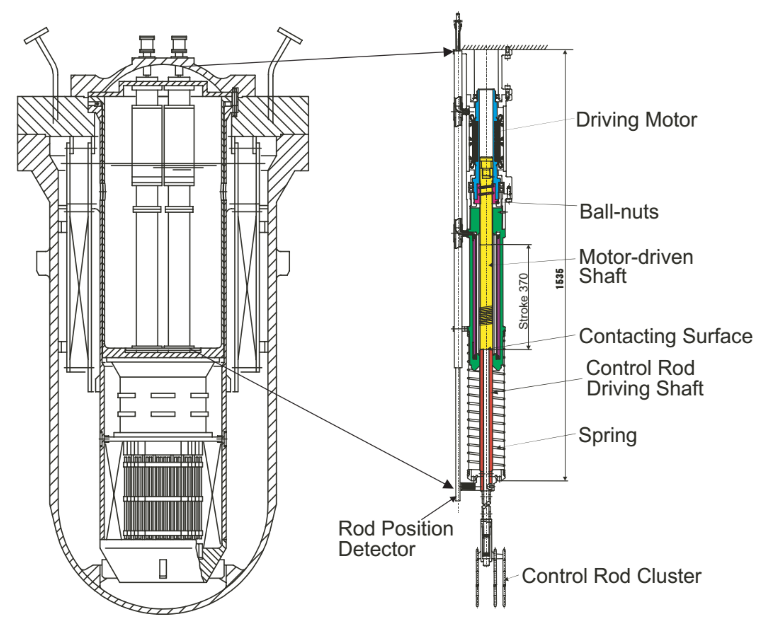
2. The Control Rod System

2.1. Control Rod System Description

The Control Rod System (CRS) (Figure 1) is an important system of a NPP, whose function is to adjust the insertion and withdrawal of control rods in the reactor core, so as to control the thermal power and, thus, the electric power generated [22,23,24,25] with a closed-loop feedback control (Figure 2). The CRS elementary scheme comprises of a sensor, a controller, a connecting network, an actuator, and a motor for rod movement, where r k , u k , y k , e k are the discrete reference, control, output, and error signals, respectively, at discrete time t k = k h [26], where h is the interval of sensor sampling and k = 0 , 1 , 2 , is a discrete integer variable as a data-sampling sequence number. The feedback control loop accounts for a total delay time τ that sums up the network transmission ( τ s c , τ c a ) and controller processing ( τ c ) delay times.
Without loss of generality, the CRS here considered comprises of (i) a typical digital Instrumental & Control (I&C) platform in single-controller mode with one CPU (for the controller module), and (ii) a typical DC motor (for the motor used to control the position of the control rods [22,27]). For the convenience of simulation, we use the discrete form of the transfer function (Equations (1) and (2) below) proposed in [26] between the DC motor and controller (where u and y are the control signal output of the controller and control rod’s relative position controlled by the DC motor (considered as the percentage of energy output), respectively, and i is the index for the simulation step):
y i = 1.944 y i 1 0.944 y i 2 + 0.004 u i 1 + 0.0039 u i 2
u i = u i 1 + 0.17 e i 0.163 e i 1

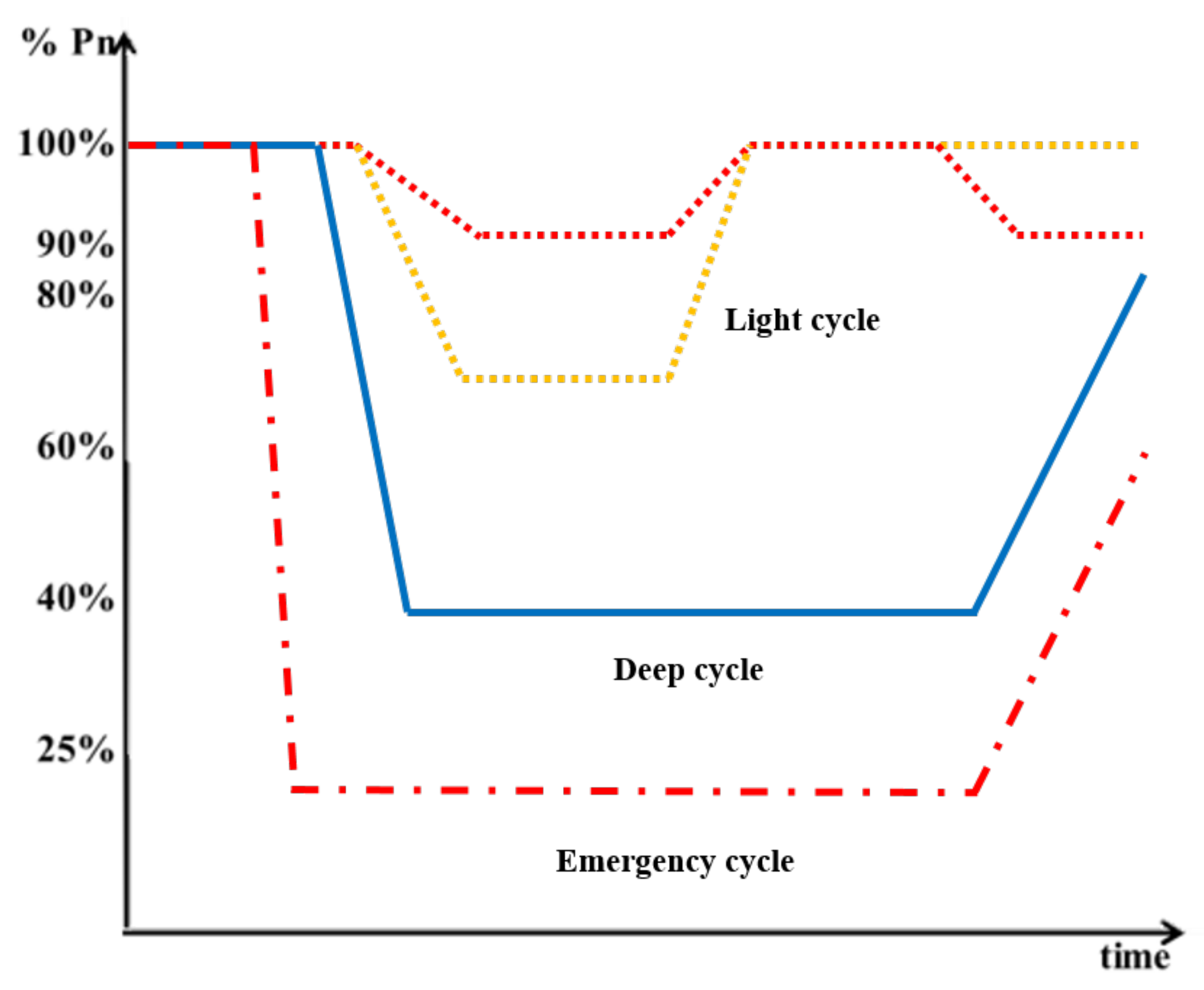
2.2. Load-Following Operation of the CRS

By definition, load-following means adjusting the electricity generation to match the expected electricity load curve [28]. A complete load-following cycle consists of a power decrease from the normal power rate ( P n ) of the CPES to a lower percentage of P n ( % P n ), followed by a ramp to re-establish the lower power level to P n [29]. As shown in Figure 3, different types of cycles can be envisaged in practical applications: “light cycles” with a limited power excursion (above 60 % P n ) (dotted line); “deep cycles” with a large variation of power (below 60 % P n ) (continuous line), and an “emergency cycle” with a large variation of power (below 50 % P n ) by a high power change rate (dashed-dotted line). For these three types of cycles, the lower power plateau can be either long or short, depending on the changes of demand on the grid side. The rate of power change from P n to % P n (and vice versa) depends on the energy CPS under analysis: in our case, we assumed a change rate of 5 % P n per second for normal load-following conditions and 20 % P n per second for a power decrease due to emergency conditions (compatible with the DC motor defined in Section 2.1) [4,22,27].
In Table 1 [30], we can see that a typical PWR reactor is estimated to perform 100,000 “light cycles” to 90 % P n , 100,000 “light cycles” to 80 % P n , 15,000 “deep cycles” to 60 % P n , 12,000 “deep cycles” to 40 % P n , and 100 “emergency cycles” to 20 % P n [4] during the plant lifetime. It results that the probability that a typical PWR NPP experiences any type of load-following cycle at each hour can be calculated (by the number of load cycles divided by total working hours in a NPP lifetime of 70 years), with results listed in the third column of Table 1.

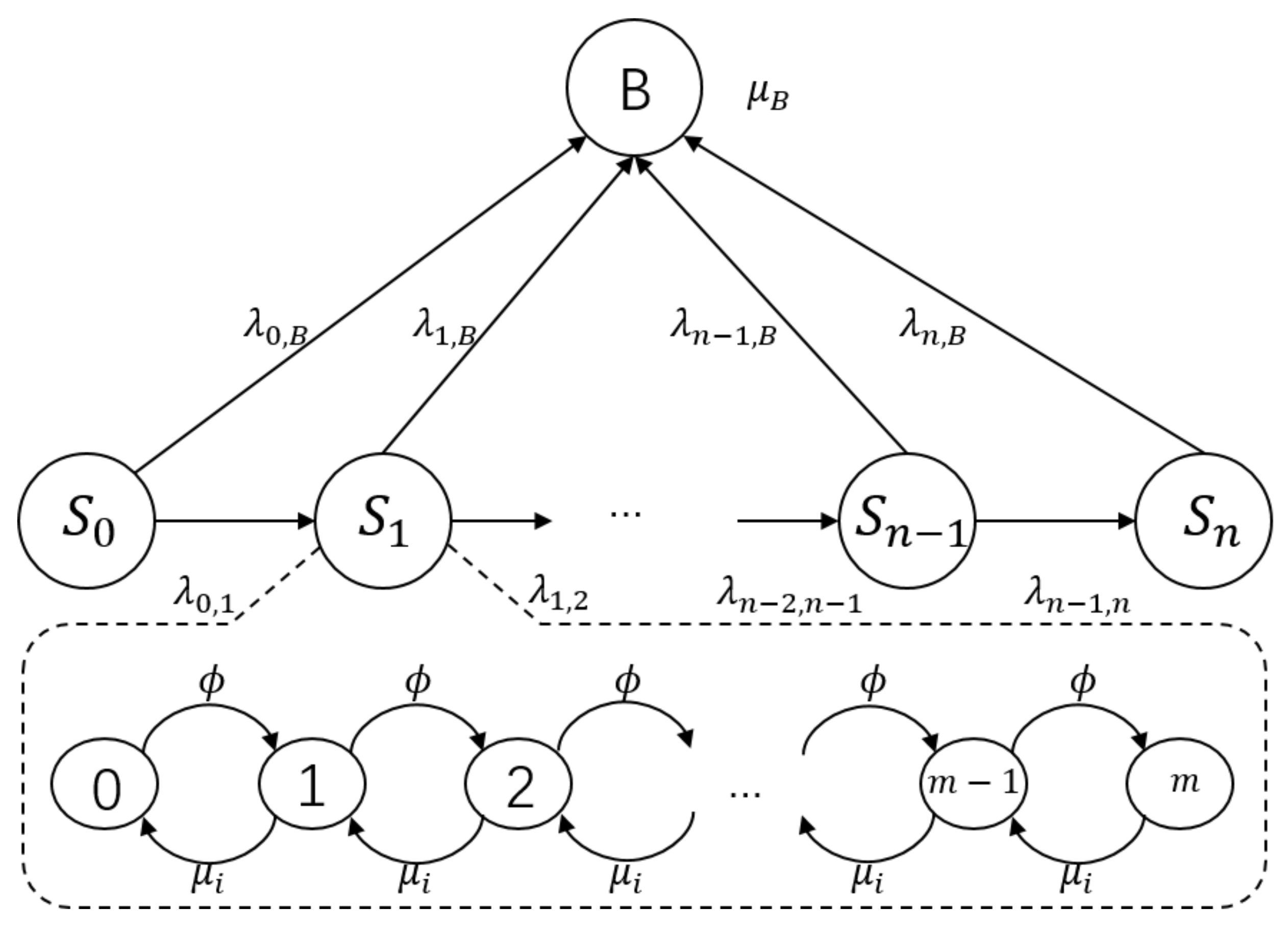
3. Modelling of Cyber Systems Aging
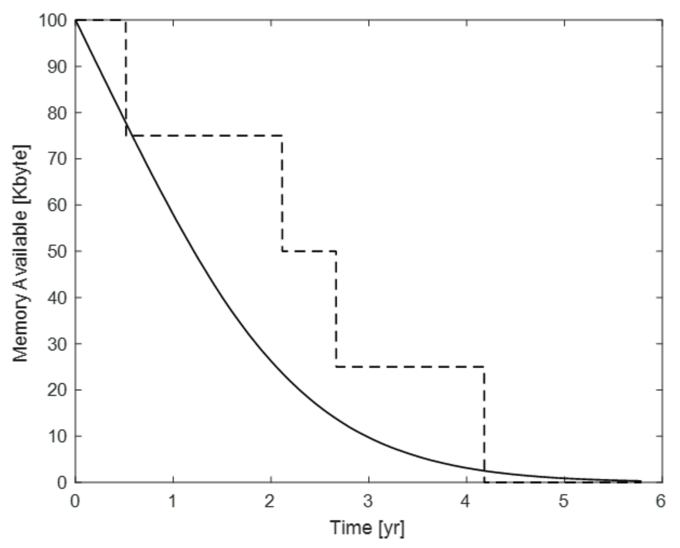
In this Section, the multi-state model of the aging process of a CPS originally presented in [15] is briefly recalled and customized for application to the CRS of Section 2.
Aging of cyber systems manifests in performance degradation and failure rate increase of the software that drives the controller [17]. Cyber system aging is caused by some specific software faults/bugs, known as aging-related bugs [18] and activated by internal/external factors, causing errors that accumulate and propagate inside the system and finally lead to aging-related failures.
Memory leakage is a typical effect of cyber aging processes caused by internal errors, like unterminated processes that shrink the available amount of physical memory [18]. With memory leakage, data-jamming can occur, due to decreasing service rates that prevent the controller from processing or delivering data and tasks in due time, which results in (i) an accumulation of data in the mission queue, (ii) an increase of the memory request, and (iii) data packet loss, when the mission queue is full [19].
As a result, the cyber system becomes blocked when the amount of memory available cannot satisfy the demand of the mission queue, significantly increasing the control delay ( τ c ) in processing data of the controller [20,31,32] and reducing controllability and stability of the controlled physical system [21], which increases risk of failure.
In the literature, modelling approaches of cyber aging are divided into two categories: measurement-based, and model-based [16,33]. With respect to measurement-based approaches, time-series analysis [34,35,36] and machine-learning methods [37,38] are used to forecast the system failure time by observing the performance degradation and resource consumption [39]. However, lacking in the generalization of systems, their data-driven characteristics make them hardly applicable to systems whose historical information is missing. With respect to model-based approaches, the cyber-aging system is commonly described as a Continuous-Time Markov Chain (CTMC) [6,40]. However, none comprehensively describes the causes, processes, and effects of cyber aging, such as service rate decrease and data-jamming.
In this work, we use CTMC to describe multiple performance degradation (i.e., service rate decrease) states embedded with a queueing model. With memory leakage, data-jamming has a higher probability of occurrence, and the system can be blocked more easily when the system cannot satisfy the memory demands, injecting high delays into the control loop which may make the system out of control. Thanks to its advantages over the mentioned approaches, (i) the chain of cyber aging phenomena is fully described; (ii) time-dependent blocking transition rates can be calculated by effects of memory leakage and the mechanism of data-jamming instead of constant transition rates with subjective assumptions, and (iii) considering the specialty of cyber aging, this model can be applied to simulate and explore system performances with high aging levels or under blocking conditions instead of directly assuming system failure.

3.1. Memory Leakage

The system performance deteriorates stochastically and eventually reaches a blocking state when the available memory cannot satisfy the demand from the mission process queue; as shown in Figure 4, the leakage degradation process can be modeled as a continuous-time Markov Chain with state space L = { S 0 , S 1 , , S n , B } , where state S 0 is the normal state, in which the system has the maximum memory capacity and performance; states S 1 S n represent increasing degradation states of decreased memory available; state B is the blocking state; λ i , i + 1 ( i = 0 , 1 , , n 1 ) is the transition rate between degradation states S i and S i + 1 ; λ i , B is the system-blocking transition rate from the i-th state S i to blocking state B (if i < j , then λ i , B < λ j , B , which means that the worse the degradation state, the larger the transition rate to the blocking state).

3.2. Data-Jamming

For each degradation state S i , assuming a data arrival rate ϕ , an exponential service rate μ i and a maximum capacity of task delivery queue equal to m, the continuous time Markov Chain of Figure 4 (below) can be used to model data-jamming, nested into the model of Figure 4 (above), where μ i denotes the different service rates in different states S i ( i = 0 , 1 , , k ) (if i < j , then μ i > μ j ), and the lowest service rate μ B is that at blocking state B.
For each state S i , the probability P j a m ( i , j ) of j data-jamming in the queue at state S i is [41]:
P j a m ( i , j ) = 1 ϕ / μ i 1 ( ϕ / μ i ) m + 1 ( ϕ μ i ) j i = 1 , 2 , , n j = 0 , 1 , , m .

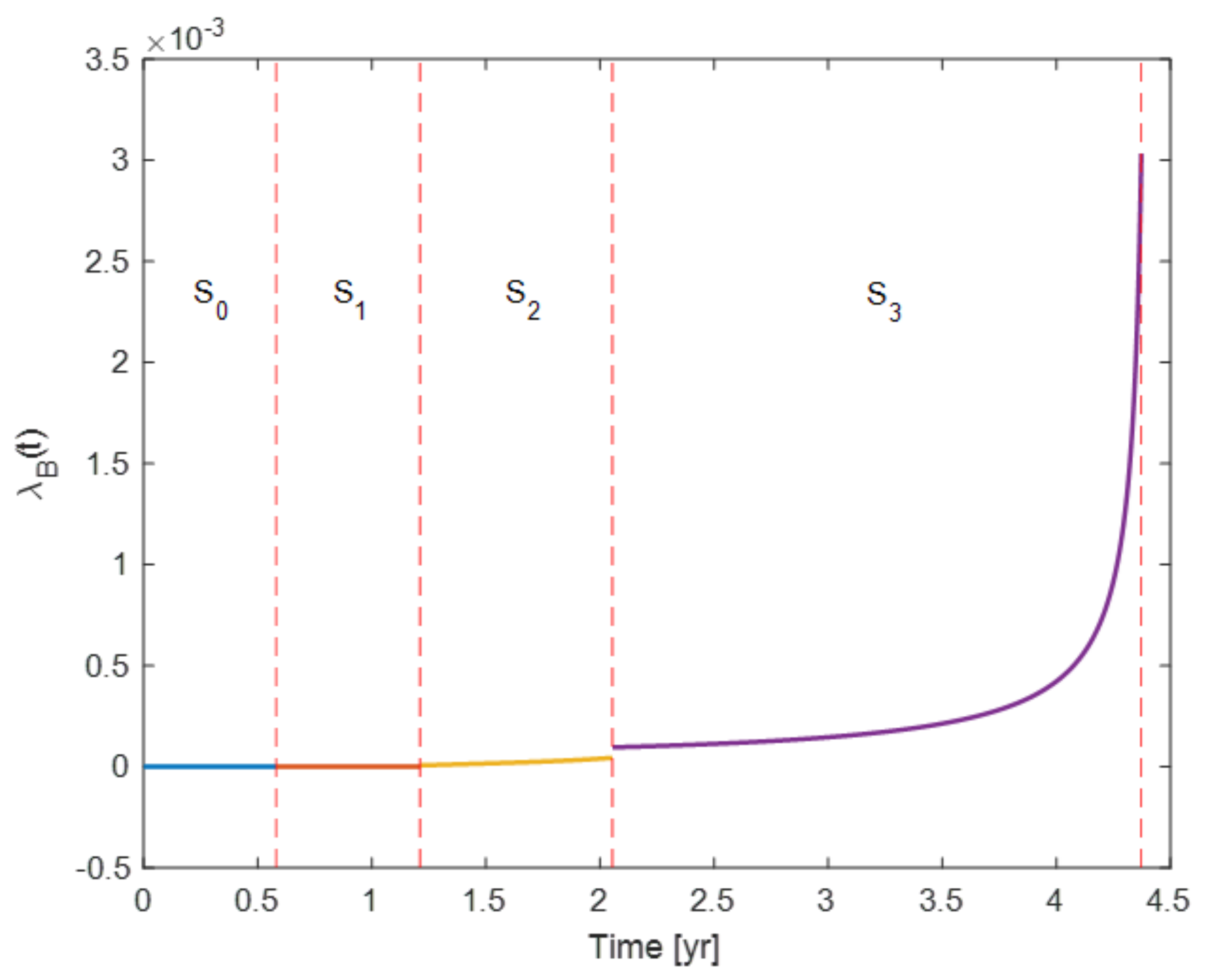
3.3. Calculation of the System-Blocking Transition Rate

As mentioned in Section 3.1, the probability of system-blocking P i , B from state S i , and the corresponding blocking transition rate λ i , B , depend on the current available memory M ( t ) and on the memory request of the mission queue, which can be calculated with the values of the model parameters listed in Table 2.
M ( t ) is estimated by assuming the transition time between degradation states ( S i and S i + 1 ) to be exponentially distributed with parameter λ i , i + 1 [16]. The Monte Carlo simulation is used to sample the transition times between states S i and S i + 1 , starting from the initial state S 0 , and the available memory in each state is recorded at each transition time; repeating the simulation N m c times, the mean value of the collected available memory at each time is taken as the available memory M ( t ) at time t. Figure 5 shows one random trial of the simulation process (dashed line).
On the other hand, to estimate the memory request of the mission queue, we need to assume that each new data comes into the queue (with maximum capacity m) with a memory request which is a continuous random variable with density function g ( x ) [40]: for any 0 < j m , let g [ j ] ( x ) be the density function for the total amount of j-independent resource requests, which is equal to the j-fold convolution of g [42].
g [ 1 ] ( x ) = g ( x ) , g [ j + 1 ] ( x ) = 0 x g [ j ] ( u ) g ( x u ) d u , j 1
Let G [ j ] ( x ) be the corresponding cumulative distribution function of g [ j ] ( x ) , G [ j ] ( x ) = 0 x g [ j ] ( u ) d u . The conditional probability ξ [ j , M ] that the system blocks with j data in the queue and M memory available upon the arrival of a new request can be calculated considering the system-blocking mechanism (i.e., the memory available cannot satisfy the memory request).
ξ [ 0 , M ] = 1 G [ 1 ] ( M ) , ξ [ j , M ] = 1 G [ j + 1 ] ( M ) G [ j ] ( M ) , 1 j m 1 ξ [ m , M ] = 1 G [ m ] ( M )
Combining the probability P j a m ( i , j ) of j data-jamming in the queue at state S i shown in Section 3.2 and the conditional probability ξ [ j , M ] of system-blocking with j data, the probability P i , B ( M ) of system-blocking at each state with M available memory can be calculated as in Equation (6) below. Remembering that M ( t ) is specific to each system, we can calculate P i , B ( t ) and the corresponding blocking transition rate λ i , B ( t ) (Figure 6) as in Equations (7) and (8) below.
P i , B ( M ) = j = 0 m P j a m ( i , j ) · ξ [ j , M ] i = 1 , 2 , , n
f i , B ( t ) = d P i , B ( t ) d t
λ i , B ( t ) = f i , B ( t ) 1 P i , B ( t )

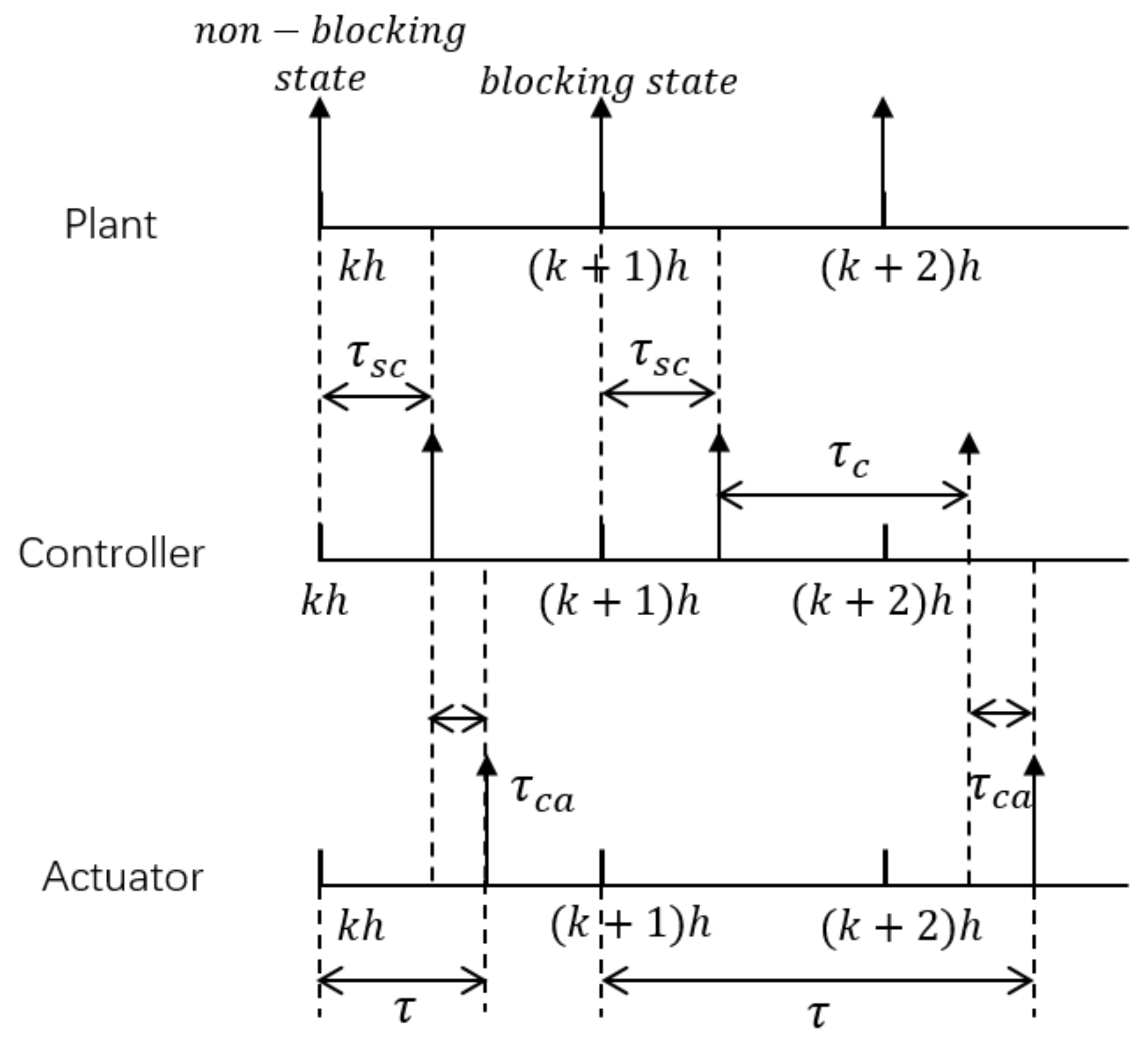
3.4. Calculation of the Control Delay

The transmission delays τ s c and τ c a of Figure 2 are usually assumed constant for a specific network structure, whereas τ c is dependent on the system state (blocking or non-blocking), and consists of the waiting time τ w a i t i n g necessary for a data packet to be processed, and in the calculating time τ c a l c u l a t i n g . When the cyber system is in a non-blocking state S 0 S n , the control delay equals to the sum of τ s c and τ c a ( τ c can be neglected); whereas when the cyber system is in the blocking state B, the low service rate causes data packet accumulation in the mission queue, significantly increasing τ c , which results in an increase of the total control delay τ [43].
τ c = τ w a i t i n g + τ c a l c u l a t i n g
τ = τ s c + τ c a , S 0 S n τ s c + τ c a + τ c , B
The signal delay calculation in a degraded CPS is sketched in Figure 7: the sensors sample the signals from the plant at the k-th sampling time; the control command signal finally reaches the actuator after delay τ : when the cyber system is in a non-blocking state S 0 S n , the total delay τ only accounts for τ s c and τ c a , commonly less than h; whereas when the cyber system is in the blocking state B, τ also accounts for τ c , making τ larger than h.

4. Reliability Analysis of the CRS

In this Section, we show the procedure to calculate the reliability of the NPP CRS described in Section 2, while being used for flexible control during load-following operations. Cyber system aging is modelled as described in Section 3.3. The failure rates of the controller and DC motor are listed in Table 3 [44,45]. It is worth mentioning that we assume failure rates of both the controller and DC motor to be constant (and their failure times exponentially distributed) even though, in the literature, the lifetime of DC motor failure times are shown to change with temperature and to obey a Weibull distribution [46]. This assumption is here justified by the fact that the CRS is assumed to operate at a constant temperature.
The CRS is considered to be failed when the system response (power output) is out of the control safety boundary, that assumed to be smaller or larger than 2 % P n . Figure 8 shows examples of normal (continuous line) and failing (dotted line) load-following operations, which are both assumed to start at t = 1 s (the safety boundaries for a 100 % P n to 60 % P n power decrease are [ 59.2 % P n ; 60.8 % P n ] (dashed-dotted line)).
The CRS is considered to undergo maintenance during the refueling outage (every 18 months), as long as the components show decreasing performance [47]. In this paper, we assume (i) to maintain the controller and DC motor, alternately, every 18 months during the refueling outage, (ii) the maintenance activity on the controller clears all accumulated aging-related bug-caused errors (such as memory leakage) and aging-related cyber failures (as good as new (AGAN)).
The procedure for the reliability assessment proceeds as follows (sketched also in Figure 9):
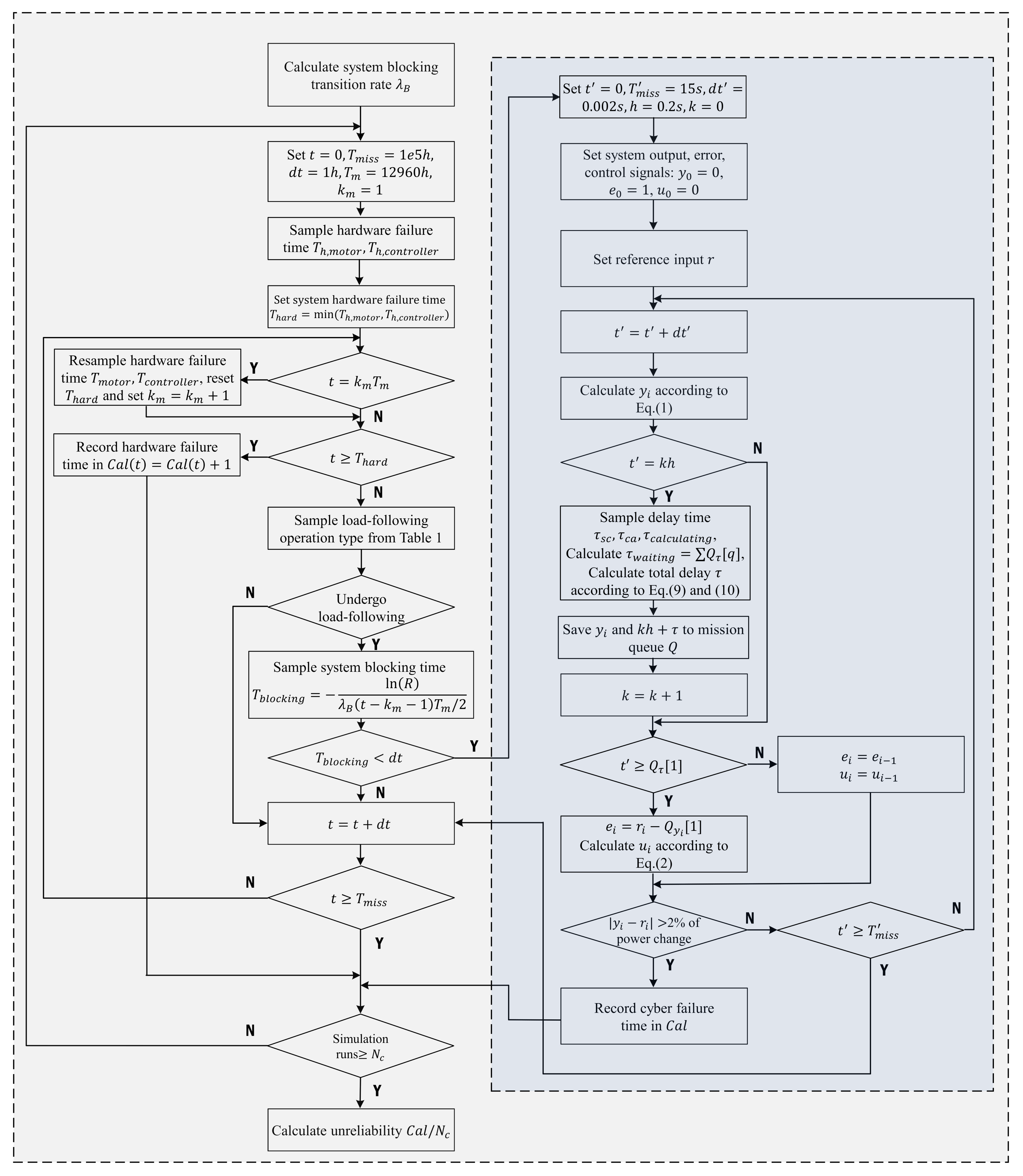
  • Calculate system-blocking transition rate λ B with the model described in [15] and the procedure summarized in Section 3.3;
  • Set: initial time t = 0 , mission time T m i s s = 10 5 h, simulation time step d t = 1 h, maintenance period T m = 12960 h (18 months) and index of maintenance cycle k m = 1 ;
  • Sample the DC motor and controller hardware failure times T h , m o t o r and T h , c o n t r o l l e r , respectively, from the exponential distributions whose rates are reported in Table 3;
  • Set the system failure time T h a r d due to hardware stochastic failures: T h a r d = min ( T h , m o t o r , T h , c o n t r o l l e r ) ;
  • Check whether the system must undergo maintenance:
    • If t = k m T m :
      (i) alternately maintain the DC motor and controller (AGAN policy), and resample the corresponding hardware failure time, T h , m o t o r or T h , c o n t r o l l e r ;
      (ii) reset the system hardware failure time T h a r d as step 4;
      (iii) set k m = k m + 1 ;
  • Check if the hardware stochastic failure time t exceeds T h a r d :
    • If t T h a r d , record system failure time due to hardware stochastic failure in the failure time counter: C a l ( t ) = C a l ( t ) + 1 , and jump to step 9;
    • If t < T h a r d :
      (i) sample load-following operation type L from the 3rd column in Table 1: if L is the index for which F L 1 < R F L , where F L = l = 0 L P l , P l is the load-following occurred probability and R is a random value sampled from the uniform distribution in [ 0 , 1 ] ; the load-following operation type L is obtained;
      (ii) sample the system-blocking time T b l o c k i n g = ln ( R ) / λ B ( t ( k m 1 ) T m / 2 ) , where R is another random value sampled from the uniform distribution in [ 0 , 1 ] ;
      (iii) if T b l o c k i n g < d t (system transits to blocking state B), start to run the load-following simulation with the type sampled in i) as following steps (a) to (h):
      (a)
      Set: load-following simulation initial time t = 0 , mission time T m i s s = 15 s, time step d t = 0.002 s, sample interval h = 0.2 s and sample iteration number k = 1 , mission queue array Q with “first in first out” processing principle;
      (b)
      Set: initial system output y 0 = 0 , error e 0 = 1 and control signals u 0 = 0 ;
      (c)
      Set: system reference input r according to different types of load-following operations (for example: r = 1.05 0.05 t ( 1 < t < 9 s ) for load-following operations from P n to 60 % P n );
      (d)
      Set t = t + d t ;
      (e)
      Calculate y i according to Equation (1)
      (f)
      Check whether new data are collected from the sensors.
      If t = k h :
      Sample the calculation delay τ c a l c u l a t i n g from the exponential distribution with parameter μ B in Table 2;
      Sample the transmission delay τ s c and τ c a from the Gaussian distributions with the parameters in Table 2;
      Calculate the data waiting time τ w a i t i n g = Q τ [ q ] , where q is the index of data waiting in the mission queue;
      Calculate the total delay time τ for the k-th sample data y i according to Equations (9) and (10);
      Save y i and k h + τ into mission queue Q as the k-th sample data and its processing end time;
      Set k = k + 1
      (g)
      Check whether the actuator time t for getting the new control signal Q y i [1] (i.e., the first data in mission queue Q) exceeds the delay time Q τ [ 1 ] :
      If t Q τ [ 1 ] , set e i = r i Q y i [ 1 ] , calculate u i according to Equation (2) and take the first data out of the mission queue;
      If t < Q τ [ 1 ] , set e i = e i 1 and u i = u i 1
      (h)
      Check whether the system output y i , which refers to the system power output, exceed 2 % of the power change above and below the reference values (i.e., the safety bounds):
      If | y i r i | > 2 % o f p o w e r c h a n g e , record the cyber failure time in the failure time counter: C a l ( t ) = C a l ( t + 1 ) , and jump to step 9;
      If | y i r i | 2 % o f p o w e r c h a n g e , repeat ( d ) to ( h ) until time t exceeds T m i s s , and finish the simulation of load-following
  • t = t + d t ;
  • Repeat steps 4 to 7 until time t exceeds T m i s s for one simulation run;
  • Run N c (e.g., 10 6 times) steps 2 to 8 and calculate the system unreliability simply as C a l / N c .

5. Results

5.1. Normal Condition

For comparison, we assess the reliability of CRS under three different modelling assumptions under normal load-following conditions (without considering 5-th row of Table 1):
  • Only hardware stochastic failures (i.e., by neglecting step 6 (i) to (iii) of the reliability assessment procedure described in Section 4);
  • Only cyber aging (i.e., by neglecting steps 3 , 4 and 5 (ii) of the reliability assessment procedure described in Section 4);
  • Both hardware stochastic failures and cyber aging.
Figure 10 shows the result of the system unreliability estimation of normal load-following operations considering the three models mentioned above (only hardware stochastic failures in continuous line, only cyber aging in dashed lines and both hardware stochastic failures and cyber aging in the dashed-dotted line). It can be seen that:
  • Hardware stochastic failures remain the principle cause of system failure;
  • Each periodic maintenance (each 18 months) efficiently reduces the system unreliability;
  • As CRS ages, longer delays are to be accommodated by the control loop, increasing the contribution of cyber aging to system failure, two years after the controller has undergone maintenance each time (with AGAN policy that clears all the aging-related errors);
  • The largest contribution of cyber aging to system failure is recorded three years after maintenance.
Effects of cyber aging on CRS are, thus, not negligible and need to be accounted for in the reliability assessment. The difference between both stochastic and cyber aging (dashed-dotted) and only stochastic (continuous) curves clearly shows the contribution of cyber aging to the overall system reliability. Cyber aging is shown to account comparatively with hardware stochastic failures, and should be only in design and for operation. It should be noticed that it is thanks to the effective periodic (AGAN) maintenance assumed, that the unreliability is maintained to a low level. Additionally, it is important to notice that the mechanism of deterioration due to cyber aging (initially silent and negligible), abruptly becomes a priority to be addressed when implementing maintenance activities.

5.2. Emergency Condition

To show the effects of cyber aging in the emergency condition, we added an emergency cycle (5-th row in Table 1) into the same simulation framework presented in Section 5.1.
Figure 11 shows the system unreliability for load-following operations under emergency conditions. When considering emergency conditions, the effects of cyber aging are magnified, further showing the need to account for it in the reliability assessment of a CPES: in the Figure 11, the difference between the highest two curves shows the significant contribution of cyber aging to the system unreliability; with respect to Figure 10 (normal conditions), cyber aging (dashed line) has a larger contribution (around 0.28 at 3 years) to the system unreliability (whereas in Figure 10 the value is around 0.08 ); periodic maintenance (every 18 months) is still an efficient method to reduce the system unreliability; as CRS ages, longer delays are introduced into the control loop (as described in Section 3), which rapidly increase the contribution of cyber-aging-caused system failure (dashed line) that can be seen two years after each AGAN periodic maintenance.
Figure 12 further shows the results of system unreliability under an emergency condition (dashed line) compared with the normal condition (dotted line), both considering hardware stochastic failure and cyber aging. The results show that emergency conditions significantly increase the system unreliability and the CRS vulnerability to cyber aging, even if the occurrence of emergency transients is very rare. During emergency conditions, the large power change needs the CRS to be highly stable and controllable: in such rare conditions, the CPES integrity is undermined because the cyber aging makes the CRS more sensitive to delays that, under normal conditions, would have led to negligible effects.

6. Conclusions

In this paper, a previously proposed multi-state model that integrates memory leakage, data-jamming, and a control delay to describe cyber system aging processes of a CPS was considered within a MC-based reliability assessment framework for CPESs typically used as the base-load, to assess the effects of cyber aging when dealing with flexible operation (e.g., load-following).
We took the CRS of a NPP as a case study, which consists of a PI controller, a DC motor, and connecting network. The result shows that: hardware stochastic failure is the main reason for system failure; the periodic maintenance (assumed AGAN) can efficiently reduce the system unreliability, for both causes of stochastic failures and cyber aging; with gradual deterioration of the control rod system and larger delays in the control loop, cyber aging starts contributing significantly, up to at most about 27 % of system unreliability; the emergency condition with a lower occurrence probability contributes more than the normal condition and increases up to, at most, about 48 % of the system unreliability.
Cyber aging can, then, be an important, non-negligible cause of unreliability in base-load CPES used for flexible operation, especially during emergency conditions. Effective preventive maintenance on the cyber system must be planned to mitigate the aging effects, together with the effective control of an energy dispatch at different base-load CPESs with different aging profiles to avoid system failure during transients.

Author Contributions

All authors have equally contributed to the work. Z.H.: conceptualization, data curation, formal analysis, investigation, methodology, software, validation, visualization and writing (original draft preparation, review and editing); F.D.M.: conceptualization, data curation, formal analysis, investigation, methodology, software, validation, visualization and writing (original draft preparation, review and editing); E.Z.: conceptualization, data curation, formal analysis, investigation, methodology, software, validation, visualization and writing (original draft preparation, review and editing). All authors have read and agreed to the published version of the manuscript.

Funding

The participation of Enrico Zio has been funded by “Smart maintenance of industrial plants and civil structures by 4.0 monitoring technologies and prognostic approaches—mac4pro”, sponsored by the call BRIC-2018 of the National Institute for Insurance against Accidents at Work—INAIL. This research was also funded by China Scholarship Council (CSC).

Conflicts of Interest

The authors declare no conflict of interest.

Abbreviations

The following abbreviations are used in this manuscript:
λ c o n t r o l l e r Controller failure rate
λ i , B Transition rate from state S i to blocking state B
λ i , i + 1 Transition rate between state S i and state S i + 1
λ m o t o r DC motor stochastic failure rate
μ B Blocking service rate
μ i Non-blocking service rate
ϕ Data arrival rate
τ Total delay time
τ c Controller processing delay time
τ c a l c u l a t i n g Calculation time of data in mission queue
τ c a Transmission delay between controller and actuator
τ s c Transmission delay between sensor and controller
τ w a i t i n g Waitting time of data to be processed in mission queue
ξ [ j , M ] Conditional probability of system-blocking with j data in the queue and M memory available
Bsystem-blocking state
C a l Counter of system failure times
d t Simulation time step
eSystem error signal
gProbability density function of memory requested by a data sample
GCumulative distribution function of memory requested by a data sample
hSensor sampling interval
iIndex of simulation steps
kData sampling sequence number
k m Index of maintenance action
MTotal memory available
mMaximum number of tasks
nNumber of degradation states
N c Number of simulation runs to calculate system unreliability
N m c Number of simulation runs to calculate memory curve
P n Normal power rate
P i , B Probability of system-blocking from state S i
P j a m Probability of data-jamming
qIndex of data waiting in the mission queue
QMission queue array
Q τ Delay time of the data waiting in mission queue Q
Q y i Value of the data waiting in mission queue Q
rSystem reference input
RRandom value sampled from uniform distribution in [ 0 , 1 ]
S i System normal or degradation state
T m Maintenance period
T b l o c k i n g system-blocking time
T h , c o n t r o l l e r Controller stochastic failure time
T h , m o t o r DC motor stochastic failure time
T h a r d System failure time due to hardware stochastic failure
T m i s s Mission time
uControl signal output
xMemory request of each task
ySystem power output
C P E S Cyber-Physical Energy System
C P S Cyber-Physical System
C R S Control Rod System
I & C Instrumental & Control
N P P Nuclear Power Plant
P W R Pressurized Wawter Reactor
R E S Renewable Energy Source

References

  1. Baheti, R.; Gill, H. Cyber-physical systems. Impact Control Technol. 2011, 12, 161–166. [Google Scholar]
  2. Lee, J.; Bagheri, B.; Kao, H.A. A cyber-physical systems architecture for industry 4.0-based manufacturing systems. Manuf. Lett. 2015, 3, 18–23. [Google Scholar] [CrossRef]
  3. Pierobon, L.; Casati, E.; Casella, F.; Haglind, F.; Colonna, P. Design methodology for flexible energy conversion systems accounting for dynamic performance. Energy 2014, 68, 667–679. [Google Scholar] [CrossRef] [Green Version]
  4. Lokhov, A. Technical and Economic Aspects of Load Following with Nuclear Power Plants; NEA OECD: Paris, France, 2011. [Google Scholar]
  5. Koutras, V.P.; Platis, A.N.; Gravvanis, G.A. On the optimization of free resources using non-homogeneous Markov chain software rejuvenation model. Reliab. Eng. Syst. Saf. 2007, 92, 1724–1732. [Google Scholar] [CrossRef]
  6. Trivedi, K.S.; Vaidyanathan, K.; Goseva-Popstojanova, K. Modeling and analysis of software aging and rejuvenation. In Proceedings of the 33rd Annual Simulation Symposium (SS 2000), Washington, DC, USA, 16–20 April 2000; pp. 270–279. [Google Scholar]
  7. Tipsuwan, Y.; Chow, M.Y. Network-based controller adaptation based on QoS negotiation and deterioration. In Proceedings of the IECON’01. 27th Annual Conference of the IEEE Industrial Electronics Society (Cat. No. 37243), Denver, CO, USA, 29 November–2 December 2001; Volume 3, pp. 1794–1799. [Google Scholar]
  8. Rajkumar, S.M.; Chakraborty, S.; Dey, R.; Deb, D. Online delay estimation and adaptive compensation in wireless networked system: An embedded control design. Int. J. Control Autom. Syst. 2020, 18, 856–866. [Google Scholar] [CrossRef] [Green Version]
  9. Di Maio, F.; Colli, D.; Zio, E.; Tao, L.; Tong, J. A multi-state physics modeling for estimating the size-and location-dependent loss of coolant accident initiating event probability. In 2017 International Topical Meeting on Probabilistic Safety Assessment and Analysis, PSA 2017; American Nuclear Society: La Grange Park, IL, USA, 2017; Volume 2, pp. 1185–1192. [Google Scholar]
  10. Lee, D.Y.; Choi, J.G.; Lyou, J. A safety assessment methodology for a digital reactor protection system. Int. J. Control. Autom. Syst. 2006, 4, 105–112. [Google Scholar]
  11. Boudali, H.; Dugan, J.B. A continuous-time Bayesian network reliability modeling, and analysis framework. IEEE Trans. Reliab. 2006, 55, 86–97. [Google Scholar] [CrossRef]
  12. Wang, W.; Di Maio, F.; Zio, E. Three-loop Monte Carlo simulation approach to Multi-State Physics Modeling for system reliability assessment. Reliab. Eng. Syst. Saf. 2017, 167, 276–289. [Google Scholar] [CrossRef] [Green Version]
  13. Wang, W.; Di Maio, F.; Zio, E. Adversarial Risk Analysis to Allocate Optimal Defense Resources for Protecting Cyber–Physical Systems from Cyber Attacks. Risk Anal. 2019, 39, 2766–2785. [Google Scholar] [CrossRef] [Green Version]
  14. Wang, W.; Cammi, A.; Di Maio, F.; Lorenzi, S.; Zio, E. A Monte Carlo-based exploration framework for identifying components vulnerable to cyber threats in nuclear power plants. Reliab. Eng. Syst. Saf. 2018, 175, 24–37. [Google Scholar] [CrossRef] [Green Version]
  15. Hao, Z.; Di Maio, F.; Zio, E. A Multi-State Model of the Aging Process of Cyber-Physical Systems. In Proceedings of the 30th European Safety and Reliability Conference, ESREL 2020, Venice, Italy, 1–5 November 2020. [Google Scholar]
  16. Du, X.; Qi, Y.; Hou, D.; Chen, Y.; Zhong, X. Modeling and performance analysis of software rejuvenation policies for multiple degradation systems. In Proceedings of the 2009 33rd Annual IEEE International Computer Software and Applications Conference, Seattle, WA, USA, 20–24 July 2009; Volume 1, pp. 240–245. [Google Scholar]
  17. Huang, Y.; Kintala, C.; Kolettis, N.; Fulton, N.D. Software rejuvenation: Analysis, module and applications. In Proceedings of the Twenty-Fifth International Symposium on Fault-Tolerant Computing, Pasadena, CA, USA, 27–30 June 1995; pp. 381–390. [Google Scholar]
  18. Grottke, M.; Matias, R.; Trivedi, K.S. The fundamentals of software aging. In Proceedings of the 2008 IEEE International Conference on Software Reliability Engineering Workshops (ISSRE Wksp), Seattle, WA, USA, 11–14 November 2008; pp. 1–6. [Google Scholar]
  19. Garg, S.; Puliafito, A.; Telek, M.; Trivedi, K. Analysis of preventive maintenance in transactions based software systems. IEEE Trans. Comput. 1998, 47, 96–107. [Google Scholar] [CrossRef]
  20. Cloosterman, M.B.; Van de Wouw, N.; Heemels, W.; Nijmeijer, H. Stability of networked control systems with uncertain time-varying delays. IEEE Trans. Autom. Control. 2009, 54, 1575–1580. [Google Scholar] [CrossRef]
  21. Åström, K.J.; Wittenmark, B. Computer-Controlled Systems: Theory and Design; Courier Corporation: North Chelmsford, MA, USA, 2013. [Google Scholar]
  22. Divandari, M.; Hashemi-Tilehnoee, M.; Khaleghi, M.; Hosseinkhah, M. A novel control-rod drive mechanism via electromagnetic levitation in MNSR. Nukleonika 2014, 59, 73–79. [Google Scholar] [CrossRef] [Green Version]
  23. Yoritsune, T.; Ishida, T.; Imayoshi, S. In-vessel type control rod drive mechanism using magnetic force latching for a very small reactor. J. Nucl. Sci. Technol. 2002, 39, 913–922. [Google Scholar] [CrossRef]
  24. Yuanqiang, W.; Xingzhong, D.; Huizhong, Z.; Zhiyong, H. Design and tests for the HTR-10 control rod system. Nucl. Eng. Des. 2002, 218, 147–154. [Google Scholar] [CrossRef]
  25. Bakhri, S. Investigation of Rod Control System Reliability of Pwr Reactors. KnE Energy 2016, 1, 94–105. [Google Scholar] [CrossRef] [Green Version]
  26. Tipsuwan, Y.; Chow, M.Y. Control methodologies in networked control systems. Control Eng. Pract. 2003, 11, 1099–1111. [Google Scholar] [CrossRef]
  27. Divandari, M.; Hashemi-Tilehnoee, M.; Asgari-Ziarati, B.; Hosseinkhah, M.; Sabagh, K. Minimizing torque ripple in a brushless DC motor with fuzzy logic: Applied to control rod driving mechanism of MNSR. Nucl. Sci. Tech. 2015, 26, 10601-010601. [Google Scholar]
  28. Lazarev, G.; Hrustalyov, V.; Garievskij, M. 1. Non-baseload Operation in Nuclear Power Plants: Load Following and Frequency Control Modes of Flexible Operation. Nucl. Energy Ser. 2018, 1, 173. [Google Scholar]
  29. Bruynooghe, C.; Eriksson, A.; Fulli, G. Load-following operating mode at Nuclear Power Plants (NPPs) and incidence on Operation and Maintenance (O&M) costs. JRC Rep. 2010, 5, JRC60700. [Google Scholar]
  30. Ludwig, H.; Salnikova, T.; Stockman, A.; Waas, U. Load cycling capabilities of german nuclear power plants (NPP). VGB Powertech 2011, 91, 38–44. [Google Scholar]
  31. Yue, D.; Han, Q.L.; Peng, C. State feedback controller design of networked control systems. In Proceedings of the 2004 IEEE International Conference on Control Applications, Taipei, Taiwan, 2–4 September 2004; Volume 1, pp. 242–247. [Google Scholar]
  32. Peng, C.; Tian, Y.C.; Tade, M.O. State feedback controller design of networked control systems with interval time-varying delay and nonlinearity. Int. J. Robust Nonlinear Control IFAC-Affil. J. 2008, 18, 1285–1301. [Google Scholar] [CrossRef] [Green Version]
  33. Bovenzi, A.; Cotroneo, D.; Pietrantuono, R.; Russo, S. Workload characterization for software aging analysis. In Proceedings of the 2011 IEEE 22nd International Symposium on Software Reliability Engineering, Hiroshima, Japan, 29 November–2 December 2011; pp. 240–249. [Google Scholar]
  34. Li, L.; Vaidyanathan, K.; Trivedi, K.S. An approach for estimation of software aging in a web server. In Proceedings of the International Symposium on Empirical Software Engineering, Nara, Japan, 3–4 October 2002; pp. 91–100. [Google Scholar]
  35. Grottke, M.; Li, L.; Vaidyanathan, K.; Trivedi, K.S. Analysis of software aging in a web server. IEEE Trans. Reliab. 2006, 55, 411–420. [Google Scholar] [CrossRef]
  36. Magalhães, J.P.; Silva, L.M. Prediction of performance anomalies in web-applications based-on software aging scenarios. In Proceedings of the 2010 IEEE Second International Workshop on Software Aging and Rejuvenation, San Jose, CA, USA, 2 November 2010; pp. 1–7. [Google Scholar]
  37. Cassidy, K.J.; Gross, K.C.; Malekpour, A. Advanced pattern recognition for detection of complex software aging phenomena in online transaction processing servers. In Proceedings of the International Conference on Dependable Systems and Networks, Washington, DC, USA, 23–26 June 2002; pp. 478–482. [Google Scholar]
  38. Alonso, J.; Belanche, L.; Avresky, D.R. Predicting software anomalies using machine learning techniques. In Proceedings of the 2011 IEEE 10th International Symposium on Network Computing and Applications, Cambridge, MA, USA, 25–27 August 2011; pp. 163–170. [Google Scholar]
  39. Cotroneo, D.; Natella, R.; Pietrantuono, R.; Russo, S. A survey of software aging and rejuvenation studies. ACM J. Emerg. Technol. Comput. Syst. (JETC) 2014, 10, 1–34. [Google Scholar] [CrossRef]
  40. Bao, Y.; Sun, X.; Trivedi, K.S. A workload-based analysis of software aging, and rejuvenation. IEEE Trans. Reliab. 2005, 54, 541–548. [Google Scholar] [CrossRef]
  41. Bolch, G.; Greiner, S.; De Meer, H.; Trivedi, K.S. Queueing Networks and Markov Chains: Modeling and Performance Evaluation with Computer Science Applications; John Wiley & Sons: Hoboken, NJ, USA, 2006. [Google Scholar]
  42. Trivedi, K. Probability and Statistics with Reliability, Queuing and Computer Science Applications; John Wiley & Sons: Hoboken, NJ, USA, 2001. [Google Scholar]
  43. Long, M.; Wu, C.H.; Hung, J.Y. Denial of service attacks on network-based control systems: Impact and mitigation. IEEE Trans. Ind. Inform. 2005, 1, 85–96. [Google Scholar] [CrossRef]
  44. Chyou, Y.P.; Yu, D.D.; Cheng, Y.N. Performance validation on the prototype of control rod driving mechanism for the TRR-II project. Nucl. Eng. Des. 2004, 227, 195–207. [Google Scholar] [CrossRef]
  45. Iida, H.; Imayoshi, S.; Morimoto, K.; Watanabe, M.; Komada, N.; Takeshita, T. Long-term stability of Sm2Co17-type magnets for control rod drive mechanism (CRDM) in a nuclear reactor. IEEE Trans. Magn. 1995, 31, 3653–3655. [Google Scholar] [CrossRef]
  46. Song, K.; Shi, J.; Yi, X.; Xie, Y.; Liu, G.; Lu, M. Accelerated Life Data Analysis for Control Rod Drive Mechanism Coil. In Proceedings of the 2019 International Conference on Sensing, Diagnostics, Prognostics, and Control (SDPC), Beijing, China, 15–17 August 2019; pp. 940–943. [Google Scholar]
  47. Greene, R. Aging assessment of BWR control rod drive systems. Nucl. Saf. 1992, 33, 87–99. [Google Scholar]
Figure 1. Structure of control rod mechanism.
Energies 14 03241 g001
Figure 2. Closed-loop control of control rod system.
Energies 14 03241 g002
Figure 3. Load-following capability by cycle type.
Energies 14 03241 g003
Figure 4. Multiple degradation states of cyber aging.
Energies 14 03241 g004
Figure 5. Decreasing available memory M ( t ) (continuous line).
Energies 14 03241 g005
Figure 6. Transition rate of system-blocking.
Energies 14 03241 g006
Figure 7. Delay of the CPS control.
Energies 14 03241 g007
Figure 8. Examples of system load-following operations.
Energies 14 03241 g008
Figure 9. Flowchart of system unreliability calculation considering cyber aging and stochastic failures.
Energies 14 03241 g009
Figure 10. Result of system unreliability under a normal condition.
Energies 14 03241 g010
Figure 11. Result of system unreliability under the emergency condition.
Energies 14 03241 g011
Figure 12. Results comparison between normal and emergency conditions.
Energies 14 03241 g012
Table 1. PWR reactor load-following capability [30].
Load CycleNumber of Load CyclesProbability
100-90-100100,000 0.163
100-80-100100,000 0.163
100-60-10015,000 0.0245
100-40-10012,000 0.0196
100-20-100 (emergency)100 1.65 × 10 4
No load-following 0.6297
Table 2. Parameters for cyber aging model.
ParameterDescriptionValue
nNumber of degradation states3
λ i , i + 1 Transition rate between states S i and S i + 1 5 × 10 5 [h 1 ]
mMaximum number of tasks10
ϕ Data coming rate50 [s 1 ]
μ 0 Service rate in state S 0 100 [s 1 ]
μ 1 Service rate in state S 1 85 [s 1 ]
μ 2 Service rate in state S 2 70 [s 1 ]
μ 3 Service rate in state S 3 55 [s 1 ]
μ B Service rate in state Blocking30 [s 1 ]
MTotal memory available100 [Kb]
xMemory request of each taskU(2,7) [Kb]
τ s c , τ c a Transmission delayN(13.1,5.7) [ms]
Table 3. Parameters for hardware stochastic failure.
ParameterDescriptionValue
λ c o n t r o l l e r Controller failure rate 8.01 × 10 6 [h 1 ]
λ m o t o r DC motor failure rate 9.50 × 10 6 [h 1 ]
Publisher’s Note: MDPI stays neutral with regard to jurisdictional claims in published maps and institutional affiliations.

