Mechanistic Grey-Box Modeling of a Packed-Bed Regenerator for Industrial Applications

Abstract

Thermal energy storage is essential to compensate for energy peaks and troughs of renewable energy sources. However, to implement this storage in new or existing industries, robust and accurate component models are required. This work examines the development of a mechanistic grey-box model for a sensible thermal energy storage, a packed-bed regenerator. The mechanistic grey-box model consists of physical relations/equations and uses experimental data to optimize specific parameters of these equations. Using this approach, a basic model and two models with extensions I and II, which vary in their number from Equations (3) to (5) and parameters (3 to 6) to be fitted, are proposed. The three models’ results are analyzed and compared to existing models of the regenerator, a data-driven and a purely physical model. The results show that all developed grey-box models can extrapolate and approximate the physical behavior of the regenerator well. In particular, the extended model II shows excellent performance. While the existing data-driven model lacks robustness and the purely physical model lacks accuracy, the hybrid grey-box models do not show significant disadvantages. Compared to the data-driven and physical model, the grey-box models especially stands out due to their high accuracy, low computational effort, and high robustness.

1. Introduction

Reaching future climate goals is a major issue in today’s society. Key elements of the transition towards more sustainable energy systems are the pervasive application of renewable energies and reduction of total energy consumption. For example, the worldwide electricity demand has increased by almost 75% from 2000 to 2018, whereas the share of renewable energies was still around 28% in 2018 [1]. However, renewable energy sources such as wind or solar energy can show high fluctuations due to their dependence on the weather. To compensate for these energy peaks and troughs efficiently, thermal energy storage is required [2]. Thermal energy storage can match intermittent heat supply with demand, leading to better use of excess heat, which is still one of today’s key challenges in the industrial sector [3]. Especially the combination of innovative storage technologies with energy optimization/management tools can significantly increase process’ efficiency. Nevertheless, for integrating thermal energy storage in new or existing processes and their use in optimization tools, reliable and accurate component models for behavior prediction are required.

Typically, modeling of physical systems is separated into two distinct approaches: white-box and black-box modeling. In white-box modeling—also called physical or first principle modeling—a model of a system is based on deterministic equations using in-depth physical knowledge. These models are usually robust, but their modeling and computational effort can be high [4]. In contrast, black-box models—also called data-driven or empirical models—are based on data. Traditional data-driven modeling approaches include ARIMA (autoregressive integrated moving average) models and regression models [5]. However, with the advances in data-driven modeling techniques, Machine Learning (ML) methods have seen increased hype in recent years. These models can independently improve through experience and are able to capture complex patterns. In contrast to physical models, data-driven models—especially using ML techniques—can lack robustness due to their non-transparent structure. Though, modeling and computational effort can be decreased compared to physical models [6].

In between these two distinct approaches of white- and black-box modeling, grey-box models are located. Grey-box models can be seen as a mixture of physical and data-driven modeling, using physical considerations/equations and data. Thus, grey-box models can benefit from both modeling approaches, being robustness and low modeling and computational effort [7].

According to Sohlberg and Jacobsen [8], grey-box models can be divided into five categories. Although most studies in the literature do not explicitly identify with one of these five categories, they still give a good overview of grey-box modeling methods:

• Constrained black-box modeling: In constrained black-box modeling, constraints based on prior knowledge–e.g., limits on a model’s output or static gain–are added to a black-box model. E.g., non-linear polynomial models were constrained by steady-state information in a three-step approach in Aguirre et al. [9].
• Mechanistic modeling: Mechanistic modeling, also called parameterized physical modeling [10], uses physical equations based on prior knowledge and optimizes parameters based on data. A systematic approach for mechanistic grey-box models was proposed in Sohlberg [11].
• Semi-physical modeling: Semi-physical modeling uses prior knowledge to transform a non-linear optimization task into a linear optimization task.
• Hybrid modeling: Hybrid modeling combines white- and/or grey- and/or black-box models. The combination can either be in series or parallel arrangement. E.g., in Thompson and Kramer [12], a model for a synthesizing chemical process is developed with a Neural Network as a black-box modeling part.
• Distributed parameter modeling: Distributed parameter modeling allows for model reduction based on moving finite elements and grey-box identification [13].

Focusing on grey-box modeling of dynamic systems in industrial applications, e.g., for thermal energy storage, the research in the literature is limited: First, Tulleken [14] determined a statistical estimation of the optimal linearly parametrized dynamic regression model, using physical knowledge and bayesian techniques. Oussar and Dreyfus [15] proposed a general methodology for mechanistic grey-box modeling and applied the approach to a dynamic industrial drying process. Cen et al. [7] investigated an identification scheme for non-linear dynamic systems using grey-box Neural Networks and applied them to a reaction wheel in a satellite attitude control system. de Prada et al. [4] identified a lack in the literature for the systematic development of dynamic grey-box models and proposed a two-step approach for developing grey-box models. Therein, physical relations were defined, and a mixed-integer-linear-programming optimization approach was used to identify suitable parameters and the remaining structure. This approach was applied to an acetone-butonal-ethanol fermentation process. Pitarch et al. [16] developed grey-box models of limited complexity for process systems, based on data reconciliation and polynomial constrained regression. As a use-case, the approach was applied to an industrial evaporation plant. Finally, in the authors’ previous works [17,18], a sensible thermal energy storage, a packed-bed-regenerator (PBR), was modeled using Neural Networks and physical considerations. Although the Neural Network models showed good performance and high accuracy, their robustness/reliability was limited due to their mainly data-driven nature.

Regarding the modeling of packed-bed thermal energy storage such as the PBR in general, a good overview of different types and modeling approaches can be found in [19,20,21] analyzes the transient response of packed-bed thermal storage. Focusing on the modeling of packed-bed thermal energy storage with gaseous flow, continuous solid phase/Schumann models [22] have been widely used in the literature. These models use a uniform temperature between fluid and solid [23]. The continuous solid phase/Schumann models were used, for example, in Zanganeh et al. [24], where the sensible part of a combined sensible-latent high temperature energy storage is modeled numerically, considering separate fluid and solid phases with variable thermo-physical properties, thermal losses, and axial dispersion by conduction and radiation. Additionally, Hänchen et al. [25] used this approach and formulated the combined convection and conduction heat transfer of a high-temperature packed-bed energy storage for air-based concentrated solar power plants as a numerical model with 1D two-phase energy conservation equations. White et al. [26] investigated the thermal wave propagation in packed-bed thermal reservoirs with numerical and theoretical analysis, focusing on thermal losses due to irreversible heat transfer. Additionally, recently, König-Haagen et al. [27] modeled a packed-bed thermal energy storage in combination with an Organic Rankine Cycle using numerical modeling based on the Schumann model. Last, this modeling approach was also applied in Hoffmann et al. [28] and compared to a single-phase model. Moreover, the continuous solid phase/Schumann models, also dispersion concentric models have been applied to packed-bed thermal energy storage with gaseous flow, e.g., in Barton [29] for the storage of solar thermal energy. Furthermore, numerical modeling is used in Odenthal et al. [23] to model a horizontal packed-bed energy storage considering regularly shaped channels with gaseous flow with a one-dimensional dispersion concentric model. Finally, [30] developed a one spatial dimension transfer model of a packed-bed thermal energy storage for simulating the performance of a combined cycle concentrated solar power plant with storage.

In contrast to existing publications, this work investigates a mechanistic grey-box modeling approach to model the PBR, with the main research goal to develop an accurate and reliable model. Within this approach, physical information about the PBR is used to determine essential physical relation/equations, and measurement data are used to optimize physical, or physically inspired parameters of these equations. This way, a physically based model is built, while using far fewer equations than a traditional white-box model. Compared to the authors’ previously published mainly data-driven and solely physical models of the PBR [17,18], the proposed mechanistic grey-box modeling approach is preliminary based on physical knowledge and uses data for refinement.

To the authors’ best knowledge, a mechanistic grey-box modeling approach has not been applied yet to model sensible thermal energy storage systems such as the PBR. Thus, as the main research goal, this work presents a novel, robust and efficient modeling method for dynamic industrial systems and in-depth investigates the mechanistic grey-box modeling approach. Additionally, the presented grey-box model is a major addition to the authors’ previous publication [18], where the PBR was modeled with a primarily data-driven modeling approach using Neural Networks and also with a purely physical modeling approach. The new mechanistic grey-box model can be seen as an in-between approach of the previously used methods, using advantages of both physical and data-driven modeling.

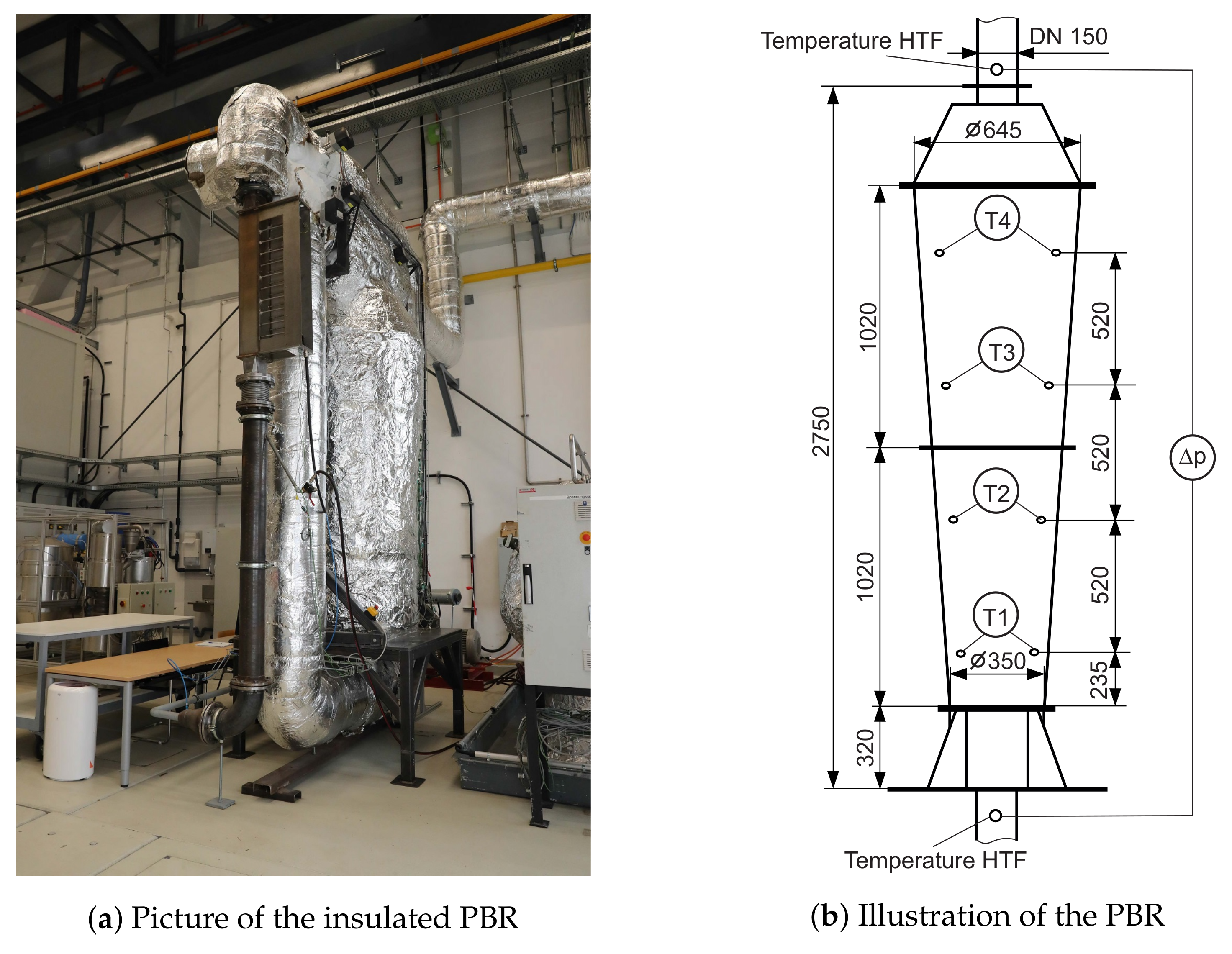
This work is organized as follows: In Section 2, the PBR and its experimental setup and operation characteristics are presented. In Section 3, the grey-box modeling approach is described, and governing equations and parameters are given. In Section 4, the results of the developed grey-box models are discussed. In Section 5, the grey-box models are compared qualitatively and quantitatively to the existing physical and data-driven model of the PBR. Finally, a conclusion and outlook is given in Section 6, followed by the Nomenclature and references.

2. Experimental Setup

As a use-case, a sensible thermal energy storage—a packed-bed regenerator (PBR)—is used. The semi-industrial scale PBR test rig is situated at the TU Wien laboratory and is depicted in Figure 1a and illustrated in Figure 1b. The main part of the PBR is the insulated conical vessel which is filled with the storage medium (SM) gravel. In this vessel, air as the heat transfer fluid (HTF) enters from the bottom and flows through the SM to the top. While charging, the HTF is heated up by an electric heater before it enters the vessel, and heat is transferred from the HTF to the SM. While discharging, cold HTF flows from the bottom to the top through the hot SM, and heat is transferred from the SM to the HTF.

For temperature measurements, the PBR is equipped with 18 temperature sensors: one at the HTF inlet and outlet (calibrated resistance temperature sensors) and four pieces of calibrated NiCr-Ni thermocouples located uniformly in each of the four horizontal layers of the vessel, according to Figure 1b. In addition, the mass flow of the HTF is measured at the inlet of the vessel with a mass flow sensor. Thus, relevant measurement data from the PBR include the HTF inlet temperature $T_{\mathrm{in}}$, the HTF outlet temperature $T_{\mathrm{out}}$, an average temperature for every horizontal layer of the vessel T1–T4, and the mass flow of the HTF $\dot{m}$. A more detailed description of the PBR test rig can be found in Michalka [31] and Hofmann et al. [18].

Measurement Series

In this work, experimental data from eight different measurement series of the PBR test rig are employed, which are displayed in

Table 1. Measurement series of the PBR.

Series	1	2	3	4	5	6	7	8
Number of Cycles	3	3	3	3	3	3	3	4
Mass Flow $\dot{m}$ in kg/h	150	150	126	150	175	200	250	146
Target Temp. Charging: $T_{\mathrm{in}}$ in ${}^{\circ }$C	310	310	230	230	230	230	230	310
Target Temp. Discharging: $T_{\mathrm{in}}$ in ${}^{\circ }$C	20	20	50	50	50	50	50	20
Max. Temp. Charging: $T_{\mathrm{out}}$ in ${}^{\circ }$C	290	200	185	185	185	185	185	265
Min. Temp. Discharging: $T_{\mathrm{out}}$ in ${}^{\circ }$C	200	150	80	80	80	80	80	50

. Each of the eight measurement series covers 3 or 4 charging/discharging cycles and includes varying HTF mass flows $\dot{m}$. The cycles are specified by a target inlet temperature $T_{\mathrm{in}}$ of the HTF for the operation modes charging and discharging. This target temperature is the desired HTF inlet temperature of the PBR to be reached by the electric heater. If the maximum (during charging) or minimal (during discharging) temperature $T_{\mathrm{out}}$ at the top of the PBR vessel is reached, the PBR switches from one operation mode to the other one.

3. Grey-Box Modeling Approach

The main aim of the developed grey-box model is the accurate and robust prediction of the HTF outlet temperature $T_{\mathrm{out}}$ of the PBR. Based on the detailed available physical knowledge and existing measurement data of the PBR test rig, a mechanistic modeling approach was chosen. In this mechanistic modeling approach, the PBR is described by physical (inspired) equations. Relevant parameters of these equations are fitted to the existing data by optimization techniques. These parameters can either be (a combination of) real physical properties, physically inspired, or empirically chosen to achieve a good fit of the model. This combination of physical and empirical modeling approaches leads to an iterative process in which essential governing equations are formulated, altered, and extended to yield an accurate and robust model.

Thus, in the first step, governing model equations are formulated, and optimization parameters are determined to create a basic model. To improve the fit of this basic model, the model is extended by additional equations and optimization parameters in the next step. In total, three different grey-box models, the basic model and two extended models, are presented and compared in this work.

3.1. General Model Features

The three developed mechanistic grey-box models of the PBR are all based on the same basic structure and use time series data of the mass flow $\dot{m}$ and inlet temperature of the HTF $T_{\mathrm{in}}$ to predict the outlet HTF temperature $T_{\mathrm{out}}$. As a modeling basis, the vessel is vertically separated into n horizontal layers, and assumed cylindrical. Each layer of the vessel is modeled by a state-space model and the layers are connected in series to form the complete model of the PBR. This way, the calculation of the HTF temperature $T_{\mathrm{out}}$ is conducted for every time-step of a measurement series.

For each of the three developed grey-box models, the models of these layers are based on different assumptions and equations. Whereas the basic model only assumes heat transfer between the HTF and SM, and heat loss to the surrounding, the extended models include additional or more detailed correlations. The following list gives an overview of the three models’ assumptions:

• Basic Model: Considering convective heat transfer between HTF and SM, and heat loss to the surrounding that is only dependent on the temperature of the SM of the current layer.
• Extended Model I–Heat Loss Dependency: Same as the basic model, including the dependency of the heat loss on the SM temperature of the previous time-steps.
• Extended Model II–Inclusion of a Wall and Non-Constant Heat Capacity: As the basic model, including an additional medium–the wall–that is set in thermal contact with the SM. Additionally, the heat capacity of the HTF and SM is not considered constant, but dependent on the temperature of the SM.

Although other modifications to the basic model were tested, they did not show relevant outcomes or significantly improved efficiency compared to the presented models. Thus, their modifications are only briefly listed for the sake of completeness. They included: Heat radiation losses, heat radiation between layers, the conical vessel shape, different part models for charging and discharging, and heat conduction between the SM of the layers. A general overview of the influences of several packed-bed thermal energy storage properties (radiation, temperature-dependent material properties, etc.) can e.g., be found in Allen [32].

3.2. Basic Grey-Box Model

In the basic grey-box model, only heat transfer between HTF and SM, and heat loss to the surrounding are considered in each layer i of the PBR vessel for every time-step k. The following procedure is used for all layers: HTF is entering layer i and flows through the SM in this layer. While charging, this leads to a warming of SM by the hot HTF and a reduction of the HTF temperature, and vice versa for discharging. Also taking into account a heat loss of the SM, this results in new temperatures of SM $T_{\mathrm{SM}}$ and HTF $T_{\mathrm{HTF}}$ in layer i and time-step k. These new SM and HTF temperatures can be used as a basis to calculate the temperatures of the subsequent layers $i+1$ and time-steps $k+1$. As the HTF flows through the solid SM, the HTF temperature depends on the HTF temperature of the previous layer $i-1$, while the SM temperature depends on the SM temperature of the previous time-step $k-1$. 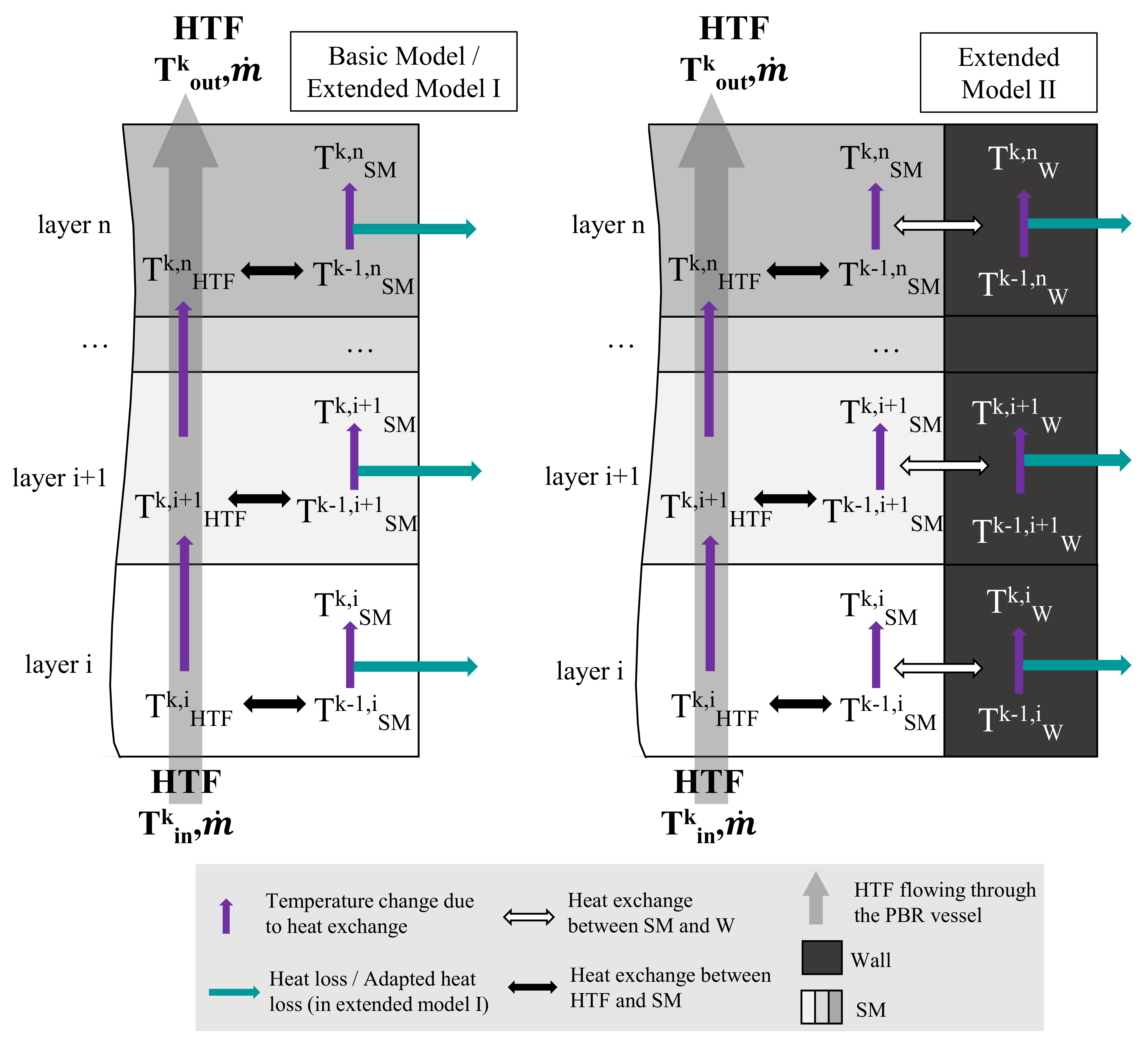This approach is also illustrated in Figure 2. Note here that the presented approach is strongly dependent on the used time-step size. However, similar to the parameters fitted by optimization, the evaluation of a fitting time-step size is part of this partly empirical modeling approach.

For the presented procedure, it is assumed that the HTF and SM in each layer i approach (but do not entirely reach) an equilibrium temperature $T_{\mathrm{eq}}$. This equilibrium temperature can be calculated by equating the heat transferred between the HTF–see Equation (1)–and SM–see Equation (2)–, according to Equation (3).

$$Q_{\mathrm{SM}}^{k,i}=(T_{\mathrm{eq}}^{k,i}-T_{\mathrm{SM}}^{k-1,i})\left(c_{\mathrm{SM}}{\rho }_{\mathrm{SM}}(1-\phi )V\right)$$

(1)

$$Q_{\mathrm{HTF}}^{k,i}=(T_{\mathrm{eq}}^{k,i}-T_{\mathrm{HTF}}^{k,i-1})(\Delta k\dot{m}{c}_{p,\mathrm{HTF}})$$

(2)

$$(T_{\mathrm{eq}}^{k,i}-T_{\mathrm{SM}}^{k-1,i})\left(c_{\mathrm{SM}}{\rho }_{\mathrm{SM}}(1-\phi )V\right)=-(T_{\mathrm{eq}}^{k,i}-T_{\mathrm{HTF}}^{k,i-1})(\Delta k\dot{m}{c}_{p,\mathrm{HTF}})$$

(3)

Considering constant values for the (isobaric) heat capacity of the HTF $c_{p,\mathrm{HTF}}$ and SM $c_{\mathrm{SM}}$, the density of the SM ${\rho }_{\mathrm{SM}}$, the porosity of the SM $\phi$, the volume of each layer V, and time-steps $\Delta k$, a new parameter ${\beta }_{\mathrm{SH}}$ can be introduced, according to Equation (4). Then, the equilibrium temperature can be formulated by Equation (5), where $\dot{m}$ is the time-dependent HTF mass flow.

$${\beta }_{\mathrm{SH}}=\frac{\Delta k{c}_{p,\mathrm{HTF}}}{c_{\mathrm{SM}}{\rho }_{\mathrm{SM}}(1-\phi )V}$$

(4)

$$T_{\mathrm{eq}}^{k,i}=\frac{{\beta }_{\mathrm{SH}}\dot{m}{T}_{\mathrm{HTF}}^{k,i-1}+T_{\mathrm{SM}}^{k-1,i}}{{\beta }_{\mathrm{SH}}\dot{m}+1}$$

(5)

This equilibrium temperature can be theoretically reached at full heat exchange between HTF and SM. However, in practice, heat exchange between HTF and SM is not completely performed, and the equilibrium temperature is not reached. To determine the actual temperatures of HTF and SM after heat exchange, the following approach is used: A new empiric parameter ${\alpha }_{\mathrm{SH}}$ is introduced that describes the share of heat exchange between HTF and SM. ${\alpha }_{\mathrm{SH}}$ = 0 stands for a complete heat exchange and ${\alpha }_{\mathrm{SH}}$ = 1 stands for no heat exchange between HTF and SM. This leads to the physically inspired equation Equation (6) to determine the temperature of the HTF. Using the parameter ${\beta }_{\mathrm{SH}}$ from Equation (4) that includes the heat transfer ratio between HTF and SM, Equation (7) can be formulated to calculate the SM temperature in layer i and time-step k.

$$T_{\mathrm{HTF}}^{k,i}=T_{\mathrm{eq}}^{k,i}-(T_{\mathrm{eq}}^{k,i}-T_{\mathrm{HTF}}^{k,i-1}){\alpha }_{\mathrm{SH}}$$

(6)

$$T_{\mathrm{SM}}^{k,i}=T_{\mathrm{eq}}^{k,i}-(T_{\mathrm{eq}}^{k,i}-T_{\mathrm{SM}}^{k-1,i}){\alpha }_{\mathrm{SH}}$$

(7)

To consider the heat loss to the surrounding that is assumed only linearly dependent on the temperature of the SM of the previous time-step, Equation (7) can be extended by the empirical parameter ${\nu }_{\mathrm{SM}}$ and the temperature difference between the surrounding $T_{\mathrm{sur}}$ and $T_{\mathrm{SM}}$ of the previous time-step. Including the heat loss, the temperature of the SM can be determined by Equation (8).

$$T_{\mathrm{SM}}^{k,i}=T_{\mathrm{eq}}^{k,i}-(T_{\mathrm{eq}}^{k,i}-T_{\mathrm{SM}}^{k-1,i}){\alpha }_{\mathrm{SH}}-{\nu }_{\mathrm{SM}}(T_{\mathrm{SM}}^{k-1,i}-T_{\mathrm{sur}})$$

(8)

Resulting, the basic model of the PBR consists of three equations, namely Equation (5) to calculate the equilibrium temperature in layer i, and Equations (6) and (8) to determine the temperatures of the HTF and SM for every time-step k in layer i after heat exchange. These equations include three parameters—${\alpha }_{\mathrm{SH}}$, ${\beta }_{\mathrm{SH}}$, and ${\nu }_{\mathrm{SM}}$—that aggregate or estimate relevant characteristics of the heat transfer between HTF and SM, and heat loss. ${\beta }_{\mathrm{SH}}$ describes the relation of heat capacity between HTF and SM according to Equation (4) and the two empirical parameters ${\alpha }_{\mathrm{SH}}$ and ${\nu }_{\mathrm{SM}}$ describe the heat transfer rate between HTF and SM, and the heat loss. Using the mechanistic grey-box modeling approach, these three parameters can be fitted by optimization methods to achieve good modeling results. Finally, to further improve this basic model, model extensions can be formulated.

3.3. Extended Grey-Box Model I—Heat Loss Dependency

The first extended model additionally considers the dependency of the heat loss on the SM temperature of previous time-steps. For this purpose, Equations (5) and (6) from the basic model are kept the same, and only Equation (8) is altered by including the moving average of the SM temperature of the previous time-steps. For the integration of the moving average, two new empirical parameters ${\nu }_{\mathrm{MA}}$ and $\gamma$ are introduced. ${\nu }_{\mathrm{MA}}$ describes the weighting of the moving average and $\gamma$ is the number of temperatures from previous time-steps used for the calculation of the moving average. The equivalent equation to Equation (8) of this extended model can be found in Equation (9).

$$T_{\mathrm{SM}}^{k,i}=T_{\mathrm{eq}}^{k,i}-(T_{\mathrm{eq}}^{k,i}-T_{\mathrm{SM}}^{k-1,i}){\alpha }_{\mathrm{SH}}-{\nu }_{\mathrm{SM}}(T_{\mathrm{SM}}^{k-1,i}-T_{\mathrm{sur}})-\frac{{\nu }_{\mathrm{MA}}}{\gamma }\sum _{j=1}^{\gamma }{T}_{\mathrm{SM}}^{k-j,i}$$

(9)

Thus, this extended grey-box model also uses three equations, Equations (5), (6) and (9). However, compared to the basic model, it includes five instead of three parameters to be fitted during optimization, being the parameters of the basic model ${\alpha }_{\mathrm{SH}}$, ${\beta }_{\mathrm{SH}}$, and ${\nu }_{\mathrm{SM}}$, and the new parameters ${\nu }_{\mathrm{MA}}$ and $\gamma$.

3.4. Extended Grey-Box Model II—Inclusion of a Wall and Non-Constant Heat Capacity

In the second extended grey-box model, in addition to the SM and HTF, another medium—the wall W—is introduced, according to Figure 2. This wall represents the steal wall (and insulation) of the PBR. In the model, the wall is set into thermal contact with the SM, allowing a horizontal temperature gradient within one layer of the PBR. Similar to the heat transfer between HTF and SM—see Equation (3)—heat transfer between SM and the wall W is described by an equilibrium temperature, according to Equation (11). Here—in accordance with Equation (4)—a parameter ${\beta }_{\mathrm{SW}}$ is introduced in Equation (10) that describes the heat capacity ratio between SM and W, using the wall’s heat capacity $c_{\mathrm{W}}$ and the auxiliary parameter $m_{\mathrm{A}}$, being the mass of the wall in one layer.

$${\beta }_{\mathrm{SW}}=\frac{c_{\mathrm{W}}{m}_{\mathrm{A}}}{c_{\mathrm{SM}}{\rho }_{\mathrm{SM}}(1-\phi )V}$$

(10)

$$T_{\mathrm{eqSW}}^{k,i}=\frac{{\beta }_{\mathrm{SW}}{T}_{\mathrm{SM}}^{k,i}+T_{\mathrm{W}}^{k-1,i}}{{\beta }_{\mathrm{SW}}+1}$$

(11)

With the equilibrium temperature between SM and W, the temperatures of the SM and W—see Equations (12) and (13)—can be determined, using a new empirical parameter ${\alpha }_{\mathrm{SW}}$ that describes the share of heat exchange between SM and W. In accordance with ${\alpha }_{\mathrm{SH}}$ described in the basic model, ${\alpha }_{\mathrm{SW}}$ = 0 stands for a complete heat exchange and ${\alpha }_{\mathrm{SW}}$ = 1 for no heat exchange.

$$T_{\mathrm{SM}}^{k,i}=T_{\mathrm{eqSW}}^{k,i}-(T_{\mathrm{eqSW}}^{k,i}-T_{\mathrm{SM}}^{k,i}){\alpha }_{\mathrm{SW}}$$

(12)

$$T_{\mathrm{W}}^{k,i}=T_{\mathrm{eqSW}}^{k,i}-(T_{\mathrm{eqSW}}^{k,i}-T_{\mathrm{W}}^{k-1,i}){\alpha }_{\mathrm{SW}}$$

(13)

In the model of the wall, the heat loss of the PBR is dependent on the temperature of the wall, the surrounding temperature $T_{\mathrm{sur}}$, and the empirical parameter ${\nu }_{\mathrm{W}}$ that describes the heat loss of the wall, leading to Equation (14) for the calculation of the wall temperature in one layer.

$$T_{\mathrm{W}}^{k,i}=T_{\mathrm{eqSW}}^{k,i}-(T_{\mathrm{eqSW}}^{k,i}-T_{\mathrm{W}}^{k-1,i}){\alpha }_{\mathrm{SW}}-{\nu }_{\mathrm{W}}(T_{\mathrm{SM}}^{k-1,i}-T_{\mathrm{sur}})$$

(14)

In addition in this extended model, the parameter ${\beta }_{\mathrm{SH}}$—describing the heat capacity ratio between HTF and SM that was assumed constant in the basic model in one layer—is now considered dependent on the temperature of the SM. This new dependent parameter is defined as ${\beta }_{\mathrm{SHT}}$ and includes the parameters for the constant ${\beta }_{\mathrm{SH}}$ and temperature dependent ${\beta }_{\mathrm{SHt}}$ heat capacity ratio, according to Equation (15).

$${\beta }_{\mathrm{SHT}}={\beta }_{\mathrm{SH}}+T_{\mathrm{SM}}^{k,i}{\beta }_{\mathrm{SHt}}$$

(15)

Thus, this extended grey-box model uses five equations, Equation (5) with the new ${\beta }_{\mathrm{SHT}}$ instead of ${\beta }_{\mathrm{SH}}$, Equations (6), (11), (12) and (14). It includes six parameters to be fitted during optimization, being ${\alpha }_{\mathrm{SH}}$, ${\alpha }_{\mathrm{SW}}$, ${\nu }_{\mathrm{W}}$, ${\beta }_{\mathrm{SW}}$, and ${\beta }_{\mathrm{SH}}$ and ${\beta }_{\mathrm{SHt}}$ that can be combined to ${\beta }_{\mathrm{SHT}}$.

3.5. Parameter Fitting–Optimization

To fit the parameters of the three developed grey-box models to the existing data, the root mean squared error (RMSE) of the model outlet $T_{\mathrm{out}}$ is optimized with the function fminsearch (using the Nelder-Mead Simplex Algorithm) in Matlab. Thus, the cost function of the optimization problem can be formulated by Equation (16), where $T_{\mathrm{out}}$ is the predicted outlet temperature of the HTF of the top layer with the grey-box models, $\overline{T_{\mathrm{out}}}$ the measured outlet temperature, and k the index for the time.

$$\sqrt{{\displaystyle {\displaystyle \sum }_k}{(\overline{T_{\mathrm{out}}}-T_{\mathrm{out}})}^2}$$

(16)

For the three developed grey-box models, different parameters are optimized with this approach, which are all dimensionless. The basic model optimizes ${\alpha }_{\mathrm{SH}}$, ${\beta }_{\mathrm{SH}}$, and ${\nu }_{\mathrm{SM}}$. The extended model with heat loss dependency adds two parameters ${\nu }_{\mathrm{MA}}$ and $\gamma$. In the extended model with the wall and non-constant heat capacity, the parameters ${\alpha }_{\mathrm{SH}}$, ${\alpha }_{\mathrm{SW}}$, ${\nu }_{\mathrm{W}}$, ${\beta }_{\mathrm{SW}}$, ${\beta }_{\mathrm{SH}}$ and ${\beta }_{\mathrm{SHt}}$ are optimized.

3.6. Simulation Procedure

Using the corresponding equations and parameters for each of the three models, the simulation of the PBR is conducted by solving the equations for every layer i and time-step k (representing one minute) of the measurement series in Matlab. For all models, the PBR is separated into 203 layers (which were empirically chosen) with a height of 1 cm, and the used measurement series include approximately 1000 to 4500 time-steps, being 16 to 75 h.

As input in every time-step, the measured inlet HTF temperature $\overline{T_{\mathrm{in}}}$ and HTF mass flow $\dot{m}$ are required. In addition, before starting the simulation, the starting values for the SM temperature in the first layer were set equal to the surrounding temperature of 22 ${}^{\circ }$C. As a result, the models predict the outlet HTF temperature $T_{\mathrm{out}}$ for all time-steps of the measurement data. In addition, the temperatures $T1$–$T4$ along the PBR vessel can be determined by the HTF temperatures of the corresponding layers.

4. Results and Discussion

For the analysis of the results, the three developed grey-box models are applied to the existing measurement data of the PBR from Table 1. Out of the eight measurement series, Series 3 is used to train the models, meaning to fit the models’ parameters to the data. The other series are used to test the models’ performance on so far unknown data. However, all series show a similar general behavior and the choice of training and test series does not affect the results considerably.

First of all, in

Table 2. Comparison of parameters and prediction accuracy of the three grey-box models.

Type of Model	Basic Model	Ext. I Heat Loss	Ext. II Wall + ${\mathit{\beta }}_{\mathbf{SHT}}$
${\alpha }_{\mathrm{SH}}$	0.722	0.155	0
${\alpha }_{\mathrm{SW}}$	-	-	0.99
${\beta }_{\mathrm{SH}}$	22.0	23.6	27.2
${\beta }_{\mathrm{SHt}}$	-	-	−0.0197
${\beta }_{\mathrm{SW}}$	-	-	4.75
${\nu }_{\mathrm{MA}}$	-	−0.00117	-
${\nu }_{\mathrm{SM}}$	0.000459	0.00174	-
${\nu }_{\mathrm{W}}$	-	-	0.00135
$\gamma$	-	166	-
Training RMSE in ${}^{\circ }$C	6.08	4.58	2.89
Test RMSE in ${}^{\circ }$C	7.68	5.51	3.03

, the dimensionless parameters and the accuracy of the results–measured by the root-mean-squared-error (RMSE) of the training and test outlet temperature $T_{\mathrm{out}}$ in ${}^{\circ }$C–of the three grey-box models are summarized. It can be seen that the test RMSE of the extended grey-box model II yields the best results with a RMSE of 3.03 ${}^{\circ }$C, followed by the extended grey-box model I with a RMSE of 4.58 ${}^{\circ }$C, and the basic model with a RMSE of 6.08 ${}^{\circ }$C. Also, the results reveal that all models extrapolate well, meaning the models can predict unknown data almost as accurate as the data they were trained with. Due to the similar behavior of the time series, this outcome was expected and can be seen by the relatively low difference between training and test RMSE, especially in the extended models I and II.

In the next step, the performance of the three grey-box models is evaluated by their prediction accuracy of the HTF temperature $T_{\mathrm{out}}$. In addition, observing the internal HTF temperatures $T1$–$T4$ allows for a more detailed analysis of the models behavior and was essential to improve and extend the grey-box models. For example, only if the temperature inside the PBR decreases steadily from $T1$ to $T4$ while charging, physically correct behavior is displayed. Although it therefore seems evident to use the temperatures $T1$–$T4$ as additional model outputs, these measurements show inaccuracies ($T3$ and $T4$ are higher than $T_{\mathrm{out}}$ in some series) and their integration in the model did not yield better outcomes. The inaccuracies are probably caused by the unequal location of the sensors in the vessel and the building of flow strains resulting in non-uniform heat exchange. Thus, these measurement were only used for the analysis of the model behavior and not integrated into the model. However, the integration of accurate measurements of $T1$–$T4$ could further improve the models’ accuracy.

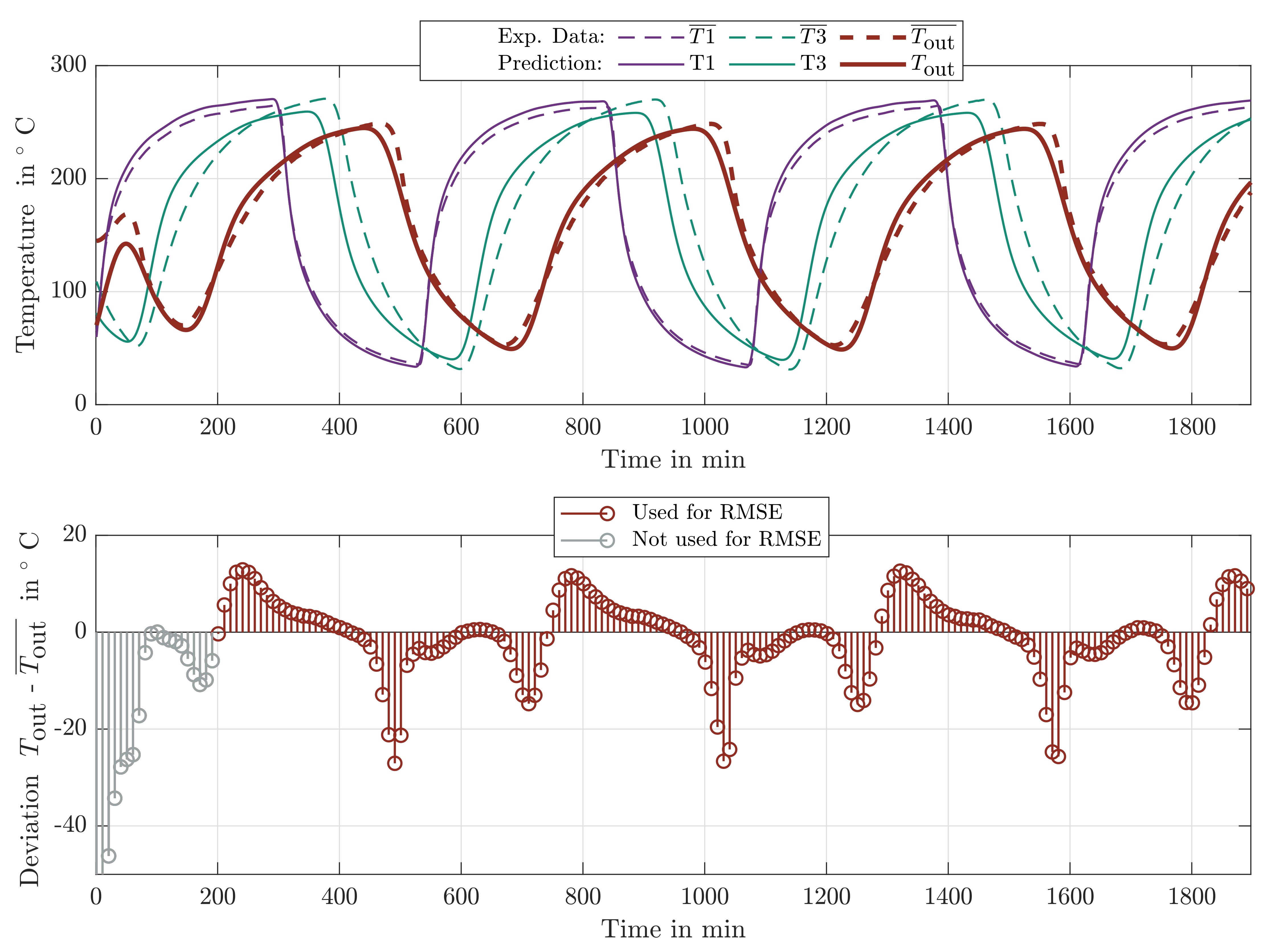
For the basic grey-box model, the measured and predicted outlet temperature and two of the internal temperatures, $T1$ and $T3$, are displayed in the upper sub-figure of Figure 3 (only two internal temperatures are displayed to limit the complexity of the figure). The lower sub-figure shows the deviation of the measured to the predicted outlet temperature. (The high deviations at the beginning of a series result from manual adjustments of the regenerator that do not reflect its actual operation behavior. Thus, the deviations at the beginning of a time series are not included in the final RMSE value.) It can be seen that during charging (rising curve), the outlet temperature and also the internal temperatures are predicted quite accurately. During discharging (falling curve) and switching between the operation modes, relatively high deviations can be seen. Moreover, the results show that the model predicts the internal temperatures physically correct (decreasing temperatures from $T1$ to $T3$ to $T_{\mathrm{out}}$) in contrast to the evidently inaccurate experimental data that shows higher values for $T3$ than $T1$. Summarized, although the basic grey-box model can approximate the general physical behavior of the PBR well, the prediction of the outlet temperature still shows significant deviations to the data.

Next, the results of the extended grey-box model I that includes the heat loss dependency are shown in Figure 4. It can be seen that this model can predict the outlet temperature (and internal temperatures) when switching between the operation modes charging and discharging more accurately than the basic model, but still shows deviations to the experimental data. Also, same as the basic grey-box model, the internal temperatures are predicted physically correct in this model. Thus, although the inclusion of the heat loss dependency increases the accuracy of the results, also this extended grey-box model can still be improved.

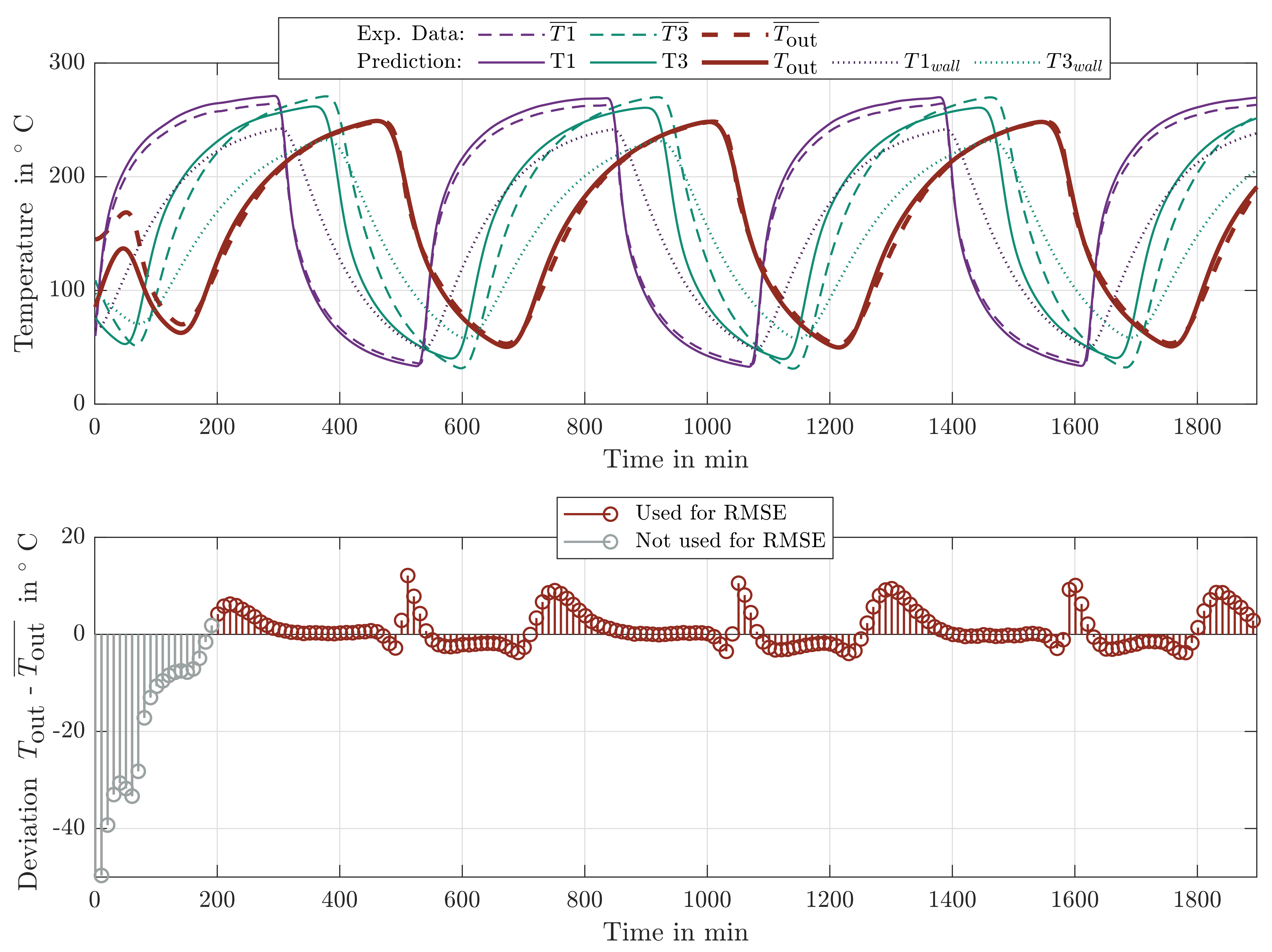
Finally, the results of the extended grey-box model II that includes a wall and non-constant heat capacity are shown in Figure 5. It can be seen that this model predicts the outlet temperature very accurately with only minor deviations and approximates the internal temperatures physically correct. For a more detailed analysis of this model, the predicted wall temperatures $T{1}_{\mathrm{wall}}$ and $T{3}_{\mathrm{wall}}$ are also displayed in Figure 5. It can be seen that the wall temperature lags the temperature of the HTF in a consistent manner. This is achieved by the additional state variable of the wall that results in a horizontal temperature gradient in each layer of the model. Although the included optimization parameters of the wall do not necessarily represent actual physical constants of the wall, they allow for a suitable approximation of the horizontal temperature distribution within the PBR.

Regarding the non-constant heat capacity ratio of the HTF and SM that is also included in this model, this adaption also slightly contributes to the excellent results of this model. This was analyzed by comparing the test RMSE of this model (RMSE = 3.03 ${}^{\circ }$C) and the basic model (RMSE = 7.68 ${}^{\circ }$C), with the test RMSE of the model only with the implementation of the wall (RMSE = 4.34 ${}^{\circ }$C) and only with the non-constant heat capacity ratio (RMSE = 7.24 ${}^{\circ }$C). Thus, it can be seen that the introduction of the wall drastically decreases the RMSE of the basic model, and that the non-constant heat capacity ratio further slightly decreases the RMSE. Also, this conclusion is amplified by the relatively close to zero value of ${\beta }_{SHt}$ in Table 2, which indicates a relatively low temperature dependence of ${\beta }_{\mathrm{SHT}}$.

Summarized, the results of the predictions with the three models lead to the following outcomes:

• All models can approximate the general physical behavior of the PBR well and display the internal temperatures physically correct. However, the extended grey-box model I, and especially the extended grey-box model II, result in significantly higher prediction accuracy than the basic model. With an RMSE of ≈3, the extended grey-box model II shows the best results.
• Especially the implementation of the wall and its additional state variable adds an essential extension to the basic grey-box model, approximating a horizontal temperature gradient in each layer.
• Although the extended grey-box model II includes two more equations and three more parameters than the basic model, the computational effort is still very low (0.12 s for predicting all measurement series on a conventional desktop computer). Thus, the slightly higher complexity does not diminish the excellent performance of this model.

Finally, to further evaluate the performance of the developed grey-box models, the models are compared to two existing models of the PBR: A purely physical model and a mainly data-driven Neural Network model.

5. Comparison of Physical, Data-Driven and Grey-Box Model

In a previous work [18], a primarily data-driven model using Neural Networks (NN) and a purely physical model of the PBR were developed. Like the grey-box models, both models aimed to accurately predict the outlet temperature $T_{\mathrm{out}}$ of the PBR. The data-driven model was based on a Recurrent Neural Network, using a specific structure to account for the time-dependent behavior of the PBR. For the creation and testing of the NN model, the same measurement series as for the grey-box models were employed. In contrast, the physical model was only based on physical relations, considering a finite difference 1D model with convective and conductive heat transfer in the mediums SM, HTF and the wall of the PBR.

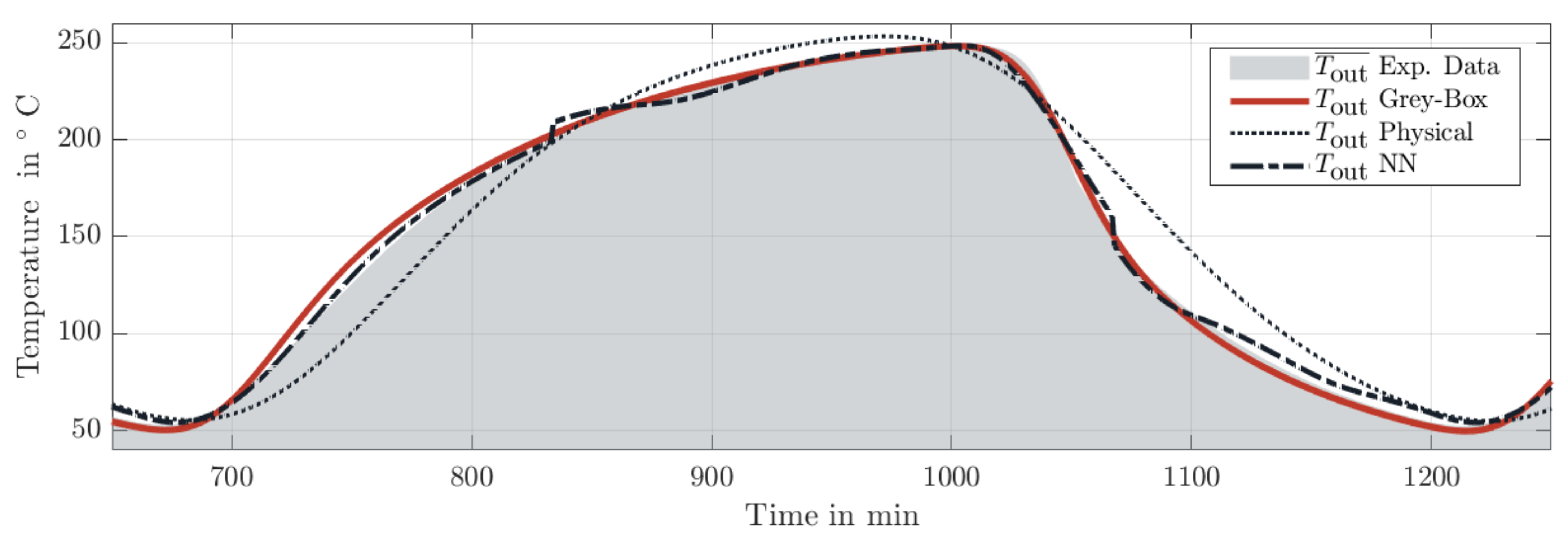
For a quantitative comparison of the different models, the prediction of the outlet temperature $T_{\mathrm{out}}$ with the physical, the data-driven NN model, and the extended grey-box model II for one charging/discharging cycle of measurement series 1 is displayed in Figure 6. It can be seen that both the physical and data-driven NN model can predict the outlet temperature of the PBR fairly accurately. Nevertheless, similar to the basic grey-box model, the physical model shows inaccuracies when switching between charging and discharging. In contrast, the NN model can predict the outlet temperature more accurately, but shows small oscillations (e.g., around time-step 840) and most importantly, it is not as robust as the physical model. This was seen by the false/nonphysical predictions of this model, if the model was trained with inaccurate experimental data. In contrast to the NN and the physical model, the developed grey-box models stand out by accurate and robust predictions. A detailed analysis of the grey-box models’ qualitative features and a short comparison with the NN and the physical model is presented below. For a more detailed description of the NN and physical model and their detailed quantitative and qualitative analysis, we refer to Hofmann et al. [18].

5.1. Qualitative Comparison

5.1.1. Modeling Effort

In the developed grey-box models, the determination of a suitable model structure was the most time-consuming step. Whereas the structure of the basic grey-box model was chosen almost right-away, the extensions of the basic model were an elaborate and iterative process. A significant number of attempts with varying physical or empirical parameters were conducted, before the extensions yielded significantly better results than the basic model, without being too complex. However, once a suitable structure was defined, its implementation, the optimization of the parameters and the actual prediction could be conducted very quickly. Compared to the existing models, the overall modeling effort for the grey-box model is a bit higher than for the data-driven NN model and lower than for the physical model. However, in the end, the modeling effort of grey-box modeling strongly depends on the application and requirements of a model.

5.1.2. Computational Effort

The developed grey-box models only use 3–5 five equations and 3–6 parameters to be optimized. Thus, the computational effort is small, leading to a maximal simulation time of 0.12 s for all eight measurement series on a conventional computer (4-core i5 processor with 8GB RAM). In contrast, the same predictions with the NN model required about 3 s and more than 100 s with the purely physical model.

5.1.3. Ability for Adaptation

For many applications, high flexibility and adaptability to changes are major modeling goals. These changes can include material or structural changes of a system, but also e.g., variations of the operation modes. Generally, physical models are able to adapt to small operational changes easily and can also conduct predictions outside their originally desired prediction-range. However, changes in material or a process’s structure might require major model adaptations. This is also true for the existing purely physical model. In contrast, data-driven models are only valid in the operation modes and ranges they were trained for. E.g., for varying operation modes, material or structural changes, the model needs to be trained with the associated new data. However, if a data-driven model’s structure can be maintained for these changes, the model can be adapted quickly and straight-forwardly with the new data. This is also valid for the existing data-driven NN model.

As a mixture of data-driven and physical models, the grey-box model allows for quick adaption to any changes. On the one hand, the grey-box model can conduct predictions outside its training range such as the physical model. On the other hand, varying operation modes, material or structural changes can be adapted straight-forwardly and quickly with the associated new data. As a further benefit of the grey-box model, in contrast to the NN model, less data for these adaptations is required. Finally, although the developed grey-box models are not directly applicable to other systems, the underlying mechanistic grey-box modeling approach offers high potential for various applications.

5.1.4. Robustness

The robustness is used as a measure for a model’s probability to generate inaccurate results. In this sense, the grey-box models—same as the purely physical model—can be considered robust. As the grey-box models are built on physical equations, their results are comprehensible and plausible, leading to only physically correct predictions. This was also emphasized by the consistently physically correct predictions of the outlet and internal temperatures of the grey-box models. In contrast, data-driven models such as the NN model are not transparent and can lead to incomprehensible/nonphysical results. As a result in the NN model, inaccurate/nonphysical data automatically led to nonphysical predictions, being higher temperatures of $T3$ than $T1$.

5.1.5. Required Knowledge and Resources

For the mechanistic grey-box modeling approach, advanced physical knowledge of the PBR was required as well as experimental data. However, in contrast to the purely physical model, fewer physical insights in the PBR were required for the creation. In comparison to the NN model, the grey-box models required smaller amounts of data. In fact, only one measurement series was enough for fitting the parameters of the grey-box models, whereas the NN model used six measurement series on average for training—and more data would have still been beneficial. Regarding resources, the development of the mechanistic grey-box models required a numerical software with optimization tools.

5.2. Summary and Discussion

Table 3. Summary of the comparison–grey-box model vs. physical model vs. data-driven NN model.

Modeling Approach	Grey-Box Model	Physical Model	NN Model
Accuracy	↑	↓	↑
Modeling Effort	$\uparrow \downarrow$	↑	↓
Computational Effort	↓	↑	↓
Effort for Small Adaptations	↓	↓	↓
Effort for Major Adaptations	↓	↑	↓
Robustness	Robust	Robust	Limited Robustness
Required Knowledge	Advanced Process Knowledge	Detailed Process Knowledge	Basic Process Knowledge
Required Resources	Numerical Software + Optimization Tools, Test & Training Data	Numerical Software, Validation Data	Numerical Software + ML Toolbox, Large Data Sets

summarizes the most important features of the grey-box models, compared to the purely physical and the data-driven NN model, where ↑ stands for high and ↓ for low, and $\uparrow \downarrow$ for moderate.

The qualitative and quantitative analysis of the results showed that the developed grey-box models—especially the extended grey-box model II—yield excellent performance, also in comparison to the existing models. The extended grey-box model II cannot only predict the outlet temperature of the PBR very accurately, but is also robust and has low computational effort. As the only drawback of this grey-box model, its modeling effort is moderate to high due to the various possibilities to combine physical considerations and data.

Finally, it can be concluded that the results of the developed mechanistic grey-box models are promising and that this approach could be a sound alternative to traditionally used numerical modeling approaches for packed-bed thermal energy storage, as described in Section 1. Especially for thermal energy storage systems with limited physical information, existing experimental data, and models that require reduced complexity (e.g., for process optimization tools), this approach stands out by accurate predictions while being significantly less complex than physical, numerical models. However, compared to purely physical models, the presented approach is not applicable for the design of systems but only for analyzing a system after its erection. Thus, as an application area, the mechanistic grey-box modeling approach could be well suited to model parts of industrial energy systems, such as the PBR, for realizing operational or design optimization of a process.

6. Conclusions and Outlook

This work analyzed the development and performance of mechanistic grey-box models for a sensible thermal energy storage, a packed-bed regenerator. The models aimed to predict the outlet temperature of the regenerator accurately and robust, using physical consideration/equations and existing data. With this mechanistic modeling approach, the regenerator was described by physical equations, and specified parameters—being either physical or physically inspired/empirical—were fitted to the data by optimization methods.

Using this approach, three mechanistic grey-box models were developed: The basic model based on 3 equations and 3 parameters, the extended model I using 3 equations and 5 parameters, and the extended model II with 5 equations and 6 parameters. The results of the models revealed that the extended grey-box model II yields the best results and can predict the PBR outlet temperature very accurately. However, all developed grey-box models can extrapolate and approximate the physical behavior of the PBR well.

Finally, compared to an existing data-driven Neural Network model and a purely physical model of the regenerator, the grey-box models show very good performance. They can benefit from high accuracy, low computational effort, low effort for adaptations, high robustness, and only small amounts of data are required. The only minor drawback of the developed grey-box models is their moderate to high modeling effort. Although the basic grey-box model could be developed very quickly, especially finding suitable model extensions and parameters was rather time-consuming. Nevertheless, it was shown that this hybrid approach—a mixture of physical and data-driven model—shows excellent qualitative and quantitative results and can be a sound alternative to traditionally used numerical modeling approaches for e.g., optimization applications.

For future work, we plan to test the grey-box models for part-load operation of the regenerator. Although further extensions for this works’ modeling purpose did not yield any significant improvements, the consideration of part-load operation or other modeling goals might require model adaptations, e.g., the implementation of accurate measurements of the internal temperatures $T1$–$T4$ or additional empirical factors. Furthermore, the approach could be applied to other industrial systems to generally evaluate the applicability of this approach to industrial process modeling.