Article

Investigation of Heat Diffusion at Nanoscale Based on Thermal Analysis of Real Test Structure

Department of Microelectronics and Computer Science, Faculty of Electrical, Electronic, Computer and Control Engineering, Lodz University of Technology, 90-924 Lodz, Poland
*
Author to whom correspondence should be addressed.
Energies 2020, 13(9), 2379; https://doi.org/10.3390/en13092379
Submission received: 18 April 2020 / Revised: 3 May 2020 / Accepted: 5 May 2020 / Published: 9 May 2020
(This article belongs to the Special Issue Latest Advances in Electrothermal Models)

Abstract

:
This paper presents an analysis related to thermal simulation of the test structure dedicated to heat-diffusion investigation at the nanoscale. The test structure consists of thin platinum resistors mounted on wafer made of silicon dioxide. A bottom part of the structure contains the silicon layer. Simulations were carried out based on the thermal simulator prepared by the authors. Simulation results were compared with real measurement outputs yielded for the mentioned test structure. The authors also propose the Grünwald–Letnikov fractional space-derivative Dual-Phase-Lag heat transfer model as a more accurate model than the classical Fourier–Kirchhoff (F–K) heat transfer model. The approximation schema of proposed model is also proposed. The accuracy and computational properties of both numerical algorithms are presented in detail.

1. Introduction

1.1. State of the Art

Nowadays, a heat transfer problem in the case of modern electronic structure is one of the most important research areas in the high-tech industry. The main reason for this fact is a significant downsizing of integrated circuits that is implemented in all modern electronic devices. Moreover, it also connects with a meaningful increase of an operation frequency of the mentioned devices. Both of these facts cause a rapid growth of a heat density generated inside such small structures. Consequently, the increased internal heat generation results in a huge increase of a temperature in critical parts of a device during its operation. It should also be highlighted that assurance of a proper cooling condition in the case of nanosized electronic structures is a non-trivial issue. Thus, all of these factors may influence an unstable operation and shorten the life cycle of an entire structure. Therefore, a thermal analysis seems to be one of the most important steps in the process of designing and developing modern electronic structures.
For a long time, heat conduction problems have been solved based on Fourier’s theory [1,2]. This approach uses the Fourier’s law and resulting Fourier–Kirchhoff (F–K) model for solids. They can be described by the following system of equations:
{ q ( x , t ) = k T ( x , t ) c v T ( x , t ) t + q ( x , t ) = q V ( x , t ) x R n ,    n N ,    t R + { 0 }
where q is a heat flux density vector; k means a thermal conductivity of investigated material; T is a function regarding temperature rise above the ambient temperature; cv means a volumetric heat capacity being a product of a specific heat of a material for a constant pressure (cp) and its density (ρ); and qV reflects the value of internally generated heat.
The classical F–K equation can also be directly derived from the classical thermodynamics for a positive-definite entropy-production rate, for which the thermodynamic state transition in a heat transfer process is extremely slow (quasi-stationary process). Therefore, the process time (t) should be longer than a system’s relaxation times.
Despite the numerous advantages of the Fourier–Kirchhoff approach, the research has shown that the application of the mentioned model may not reflect real phenomena [3,4,5]. One of its biggest disadvantages is an assumption considering the infinite speed of heat propagation. Apart from that, an instantaneous change of a temperature gradient or a heat flux should also be emphasized as a non-physical behavior postulated by the investigated theory. None of them, especially in the case of electronic structure with physical dimensions in nanometer-scale, has been empirically confirmed [6,7]. Thus, a thermal model including improvements of the F–K approach should be used instead of the classical theory.
The thermodynamic state is nonequilibrium in a fast transient process where time is comparable with the system relaxation times (e.g., an Umklapp phonon–phonon scattering process relaxation time in semiconductors [8,9]). The extended irreversible thermodynamic (EIT) can be applied to describe this kind of heat transfer system, assuming the second order the Taylor series expansion of entropy in EIT [10,11]. As a consequence, in mid-1990s, the new Dual-Phase-Lag (DPL) model was introduced by Tzou [12,13].
This model is an advanced version of an approach based on the Fourier–Kirchhoff theory and includes so-called time lags describing the time needed to change the temperature gradient, as well as the heat flux density. Each change is reflected by a separate lag value: a temperature time lag (τT) and a heat flux time lag (τq), respectively. The mathematical description of analyzed model can be presented in the form of the following system of equations:
{ q ( x , t ) = c v T ( x , t ) t + q V ( x , t ) k τ T T ( x , t ) t + τ q q ( x , t ) t = k T ( x , t ) q ( x , t ) x R n ,    n N ,    t R + { 0 }
The other general approach can be derived by using the General Equation for Non-Equilibrium Reversible-Irreversible Coupling (GENERIC) equation proposed in 1997 by M. Grmela and H. C. Öttinger [14,15,16]. This approach can be useful to obtain a model for the Monte Carlo simulation of modern nanostructures [17] and also for deterministic approaches [18]. Apart from that, an approach known as Guyer-Krumhansl-type heat conduction [19,20] can be also used. Moreover, the research presented by Pop et al. [21], related to heat generation and transportation problems in nanosized transistors, is also worth considering.
Let us consider, more precisely, one of the most common heat transfer models for electronic structures—the DPL model (Table 1a—left column), the ballistic-conductive heat transfer model (Table 1b—left column), and the model proposed in this paper, the DPL model with fractional order of the temperature function space derivative based on the Grünwald–Letnikov theory (Table 1c—left column). Suppose also an isotropic medium parameter properties and idempotent equations parameters k > 0, cv > 0, k21, k12, τT, τq, τQ, etc. To simplify the analysis, the Taylor-series expansions mapping into a function with time delay is considered, as presented in Equation (3). The terms of higher orders are neglected.
f ( x , t ) + τ f ( x , t + τ ) t f ( x , t + τ )
Then, time delayed PDEs are obtained and presented in the right column of Table 1. In the first case (Table 1a—right column), the state is appointed by using a gradient of a heat flux (−k∙ΔT) delayed by τT-τq. It should be emphasized that results produced by the DPL model are consistent with many experiments and measurements at nanoscale (for more, see [9]).
In the case of the ballistic-conductive heat transfer model (Table 1b), the rate of value temperature T(x, t + τq) change at t+ τq and x is dependent on a gradient of heat flux (−k∙ΔT) at the current time (t), increased by a difference of growth rate of the averaged value of temperature (T) over the infinitesimal neighborhood of point x and the value of temperature (T) in this point, both from the past time (tτQ):
D T ( x , t + τ q ) k Δ T ( x , t ) D t + | c v k 12 k 21 | D Δ T ( x , t τ Q )
where D(∙) is the difference operator (“change in”) corresponding to changes for Dt→0 and also for k12k21 ≤ 0. Therefore, the temperature T(x, t + τq) dynamic is additionally intensified by the dynamics of the rate of heat flux gradient (∂ΔT(x, tτQ)/∂t) in the past time (tτQ).
The approach proposed in this work is based on the temperature T(x, t + τq) dynamic control, using the fractional order of Laplace operator (GLΔαx) in the DPL model (Table 1c—right column). The integral or differential behavior of this operator and time–space discretization scheme is obtained by the value of parameter αx. The application of the fractional derivative can be interpreted as an inhomogeneous space for the heat transfer in relation to the local energy distribution (interpreted as temperature at nanoscale) in infinitesimal neighborhood of considered point. Therefore, the infinitesimal distance in Laplacian is modulated in relation to the temperature distribution around the considered point at nanoscale. The physical interpretation of the fractional derivatives is also presented in [22,23,24,25].
Hence, the proposed model (and proposed time–space scheme) is a link between experimentally confirmed DPL mesoscopic model with the ballistic heat transport model with dynamic temperature changes’ intensification useful for quasi 1-D nanostructures and for radiative heat transport without phonon collisions (e.g., metal nanowires and ultra-thin metal–oxide films).
One of the biggest advantages of the DPL approach is a universality of its application. It can be used in the case of parabolic partial differential equations, as well as for hyperbolic ones. It means that the Dual-Phase-Lag model can successfully replace the classical model based on parabolic Fourier–Kirchhoff differential equation. Of course, the DPL approach also has some disadvantages. For example, it is characterized by a bigger complexity than F–K model, what results in longer time needed for computational simulation results, especially in the case of complex structures. However, this issue will not be investigated in this paper.
The crucial achievement described in this paper is the application of the Grünwald–Letnikov fractional space-derivative in Dual-Phase-Lag heat transfer model to more accurate modeling of delays and modulation of Laplacian in relation to the temperature distribution around the considered point. This approach seems to be beneficial to represent real heat transfer behavior at the nanoscale. The proposed solution is more accurate than the F–K heat transfer model. The computation time reduction is also obtained in comparison to the DPL model. Mentioned features will be demonstrated by using a special test nanostructure developed in microelectromechanical system (MEMS) technology.
The structure of the paper is as follows. Primarily, a description of investigated real test structure is prepared. Then, analyses related to mathematical modeling of the temperature distribution inside the test structure are included. The structure’s discretization method is considered, as well. Key components of authors’ approach, i.e., DPL model approximation scheme and heat transfer enhancement (including Grünwald–Letnikov fractional derivative and its application), are described in Section 2.3 and Section 2.4. Next, simulation results are demonstrated and compared to real measurements described in [32,33]. Finally, results are discussed, and the research is summarized.

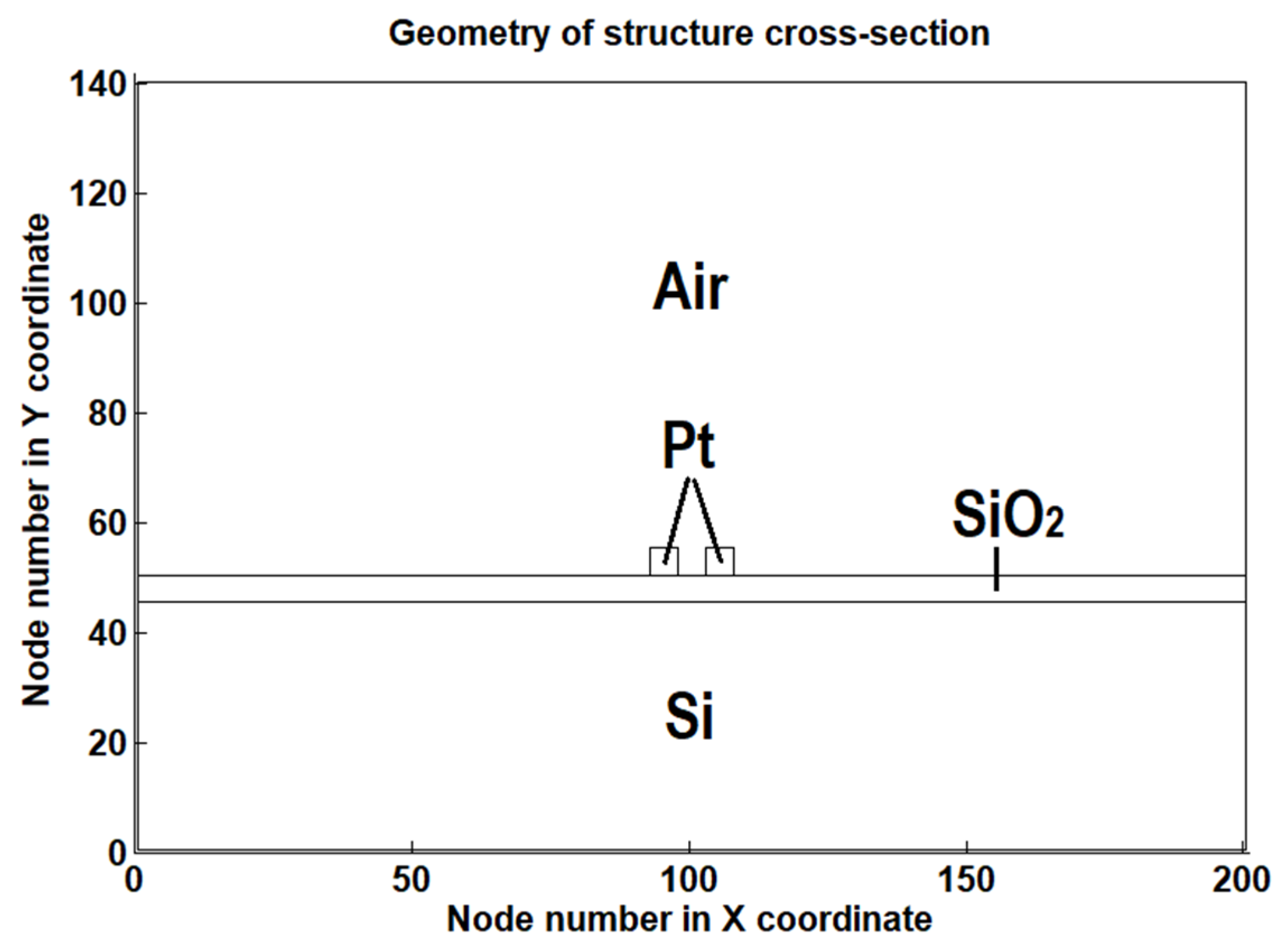
1.2. MEMS Test Structure Description

The MEMS test nanostructures were manufactured in the Polish Institute of Electron Technology. The structure consists of two parallel platinum resistors, which have lengths equal to 10 µm. The cross-sectional area of each resistor is a 100 nm square. Moreover, the distance between both resistors is also equal to 100 nm. They are placed on a thin layer of silicon dioxide, with a thickness of 100 nm. All layers are stacked on a 0.5 mm thick silicon wafer. A more detailed structure description can be found in Janicki et al. [33].
The test structure was bonded to a metal-core PCB characterized by high thermal conductivity. Moreover, the structure was connected to a biasing circuit, using high-frequency coaxial cables that were mounted to a tiny Hirose U.FL connector attached to the silicon die. Real photos of the analyzed structure, as well as the control circuit, are included in Janicki et al. [32,33].
During the measurement process, one of platinum resistors played a role of a heater, while the second one served as a temperature sensor. A detailed description of the measurement process of the test structure and obtained results is presented in [32,33].

2. Mathematical Description of Proposed Methodology

2.1. General Description

Thermal simulation was performed for the two-dimensional cross-sectional area of the investigated structure in the middle of the resistors’ length. To obtain the temperature simulation results, the DPL model, Equation (2), was used. In order to make the analysis more effective, the system of Equation (2) was transformed to an equivalent form, presented below, for two-dimensional space [34]:
c v τ q 2 T ( x , y , t ) t 2 + c v T ( x , y , t ) t k τ T Δ T ( x , y , t ) t k Δ T ( x , y , t ) = q V ( x , y , t ) x , y R ,    t R + { 0 }
The Laplacian of a temperature function ΔT was approximated by using the Finite Difference Method (FDM) according to the following formulas:
Δ T ( x , y , t ) = 2 T ( x , y , t ) x 2 + 2 T ( x , y , t ) y 2 ,                     x , y R ,    t R + { 0 }
2 T ( x , y , t ) x 2 T ( x + Δ x , y , t ) 2 T ( x , y , t ) + T ( x Δ x , y , t ) ( Δ x ) 2 , x , y R ,    t R + { 0 }
2 T ( x , y , t ) y 2 T ( x , y + Δ y , t ) 2 T ( x , y , t ) + T ( x , y Δ y , t ) ( Δ y ) 2 , x , y R ,    t R + { 0 }
Thus, considering the same difference between nodes in both axes, i.e., Δx = Δy, Laplacian ΔT can be approximated in the following way:
Δ T ( x , y , t ) T ( x + Δ x , y , t ) + T ( x , y + Δ x , t ) 4 T ( x , y , t ) + T ( x Δ x , y , t ) + T ( x , y Δ x , t ) ( Δ x ) 2 , dla     x , y R ,    t R + { 0 }
On the basis of this methodology, the authors’ method for structure discretization and FDM matrices generation was proposed. Moreover, taking into consideration the proposed approximation, the DPL equation, in the form of Equation (5), has become an ordinary differential equation of a time variable. Finally, the prepared matrix system of equations was solved for different points of time, using a class of Backward Differentiation Formulas (BDF) [35,36,37,38].
In the following subsections, the structure discretization, as well as the proposed discretization scheme for DPL model describing the temperature distribution in the cross-sectional area of investigated test structure, is characterized in detail.

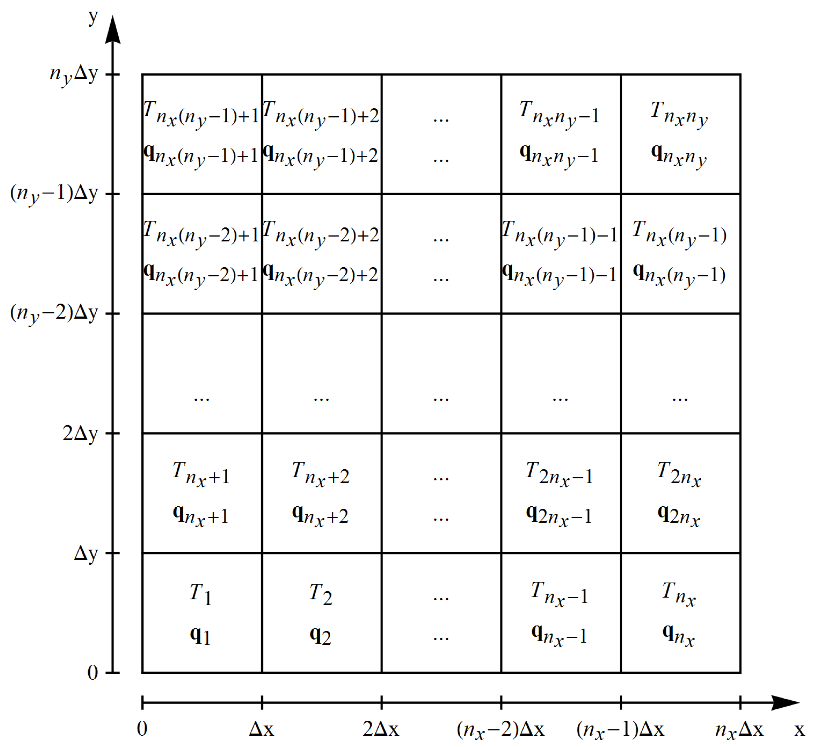
2.2. Structure Cross-Sectional Area Discretization

Primarily, the investigated cross-sectional area of the structure, as presented in Figure 1, was discretized by using two-dimensional discretization mesh characterized by the following formulas [34]:
q k ( t ) = q ( x , y , t ) ,           x = i Δ x ,     y = j Δ y
T k ( t ) = T ( x , y , t ) ,           x = i Δ x ,     y = j Δ y
i ∊ {1, 2,…, nx}, j ∊ {1, 2,…, ny}, k ∊ {1, 2,…, nxny}
where nx and ny describe a number of discretization nodes in the x-axis and y-axis, respectively. On the other hand, the product nxny reflects the entire number of nodes used to discretize the structure’s cross-section.
Nodes are numbered from the left to the right side, along the x-axis. After reaching the last point in a single row, the next part of the structure, being the nearest row from the top of the current row, was taken into consideration and numbered in the same way. Thus, node no. 1 was placed in the left bottom corner of the structure, while the node with the highest possible number, equal to nxny, was located in the top right corner. The graphical representation of used discretization mesh for analyzed cross-section of the test structure, as well as the way mesh nodes were numbered, is demonstrated in Figure 2. It is also worth highlighted that the distance between nodes in both dimensions was set to 10 nm.

2.3. Dual-Phase-Lag Approximation Scheme for Test Structure

In order to obtain the solution of temperature distribution problem inside the investigated cross-sectional area of the structure, the Dirichlet boundary conditions were considered at the bottom, while left, right and the top parts have been modeled using Neumann boundary conditions. Described situation can be characterized by the following equations:
T k ( t ) = 0 ,            t R + { 0 } ,     k { 1 , 2 , 3 , , n x }
q k ( t ) = 0 ,     t R + { 0 } ,     k { n x + 1 , 2 n x + 1 , , ( n y 1 ) n x + 1 } { n x , 2 n x , , ( n y 1 ) n x } { ( n y 1 ) n x + 1 , ( n y 1 ) n x + 2 , , n y n x }
Considering imposed boundary conditions and the FDM assumptions, the DPL model can be explained by the following system:
{ M T ¨ ( t ) + D T ˙ ( t ) + K T ( t ) = b u ( t ) y ( t ) = c T T ( t )            t R + { 0 }
where index T means a transposition, while T , T ˙ , and T ¨ are nxny-element vectors reflecting the temperature function and its first and the second time derivatives, respectively. Moreover, taking into account the way of nodes numbering, matrices Idiag, MFDM, M, D, K, and cT; vectors cv, k, τq, τT, b, and y; and the function u(t) may be reflected as indicated below:
I d i a g , M F D M , M ,    D ,    K , c T R n x n y × n x n y , c v , k , τ q , τ T b , y R n x n y ×    1 ,    u R
M F D M = [ 3 1 0 1 0 0 0 0 0 1 4 1 0 1 0 0 0 0 0 1 4 0 0 1 0 0 0 1 0 0 4 1 0 1 0 0 0 1 0 1 4 1 0 1 0 0 0 1 0 1 4 0 0 1 0 0 0 1 0 0 3 1 0 0 0 0 0 1 0 1 3 1 0 0 0 0 0 1 0 1 2 ]
M = diag ( τ q ) diag ( c v ) I d i a g
D = diag ( c v ) I d i a g 1 ( Δ x ) 2 repmat ( τ T ) repmat ( k ) M F D M
K = 1 ( Δ x ) 2 repmat ( k ) M F D M
b = a [ 0 0 1 1 0 0 ] T ,          a R +
c = I d i a g
where Idiag is an identity matrix, operator ◦ reflects matrices multiplication resulting in a Hadamard product, and matrix function diag (∙) creates a diagonal matrix from a vector, while Matlab repmat function replicates a given vector and composes a matrix of required dimensions. It is also worth highlighting that non-zero values in vector b are observed only in the case of mesh nodes characterizing a heating area.
The system in Equation (14) of differential equations of the second order was equivalently transformed into the following system of the linear first-order equations [39]:
{ E T ¯ ˙ ( t ) = A T ¯ ( t ) + B u ( t ) y ( t ) = C T T ¯ ( t )               t R + { 0 }
where T ¯ and T ¯ ˙ are 2∙nx∙ny-element vectors. The first part of vector T ¯ consists of elements of vector T, while its second part includes elements of T ˙ . On the other hand, the first and the second parts of the vector T ¯ ˙ consists of elements of vectors T ˙ and T ¨ , respectively. Moreover, matrices E, A, B, and CT can be represented in the following way [39,40]:
E = [ I d i a g Θ Θ M ] ,    A = [ Θ I d i a g K D ] ,    B = [ Θ 1 b ] ,    C = [ c Θ Θ c ]
where Θ and Θ1 are null matrices. Moreover, we get the following:
E , A , C T R 2 n x n y × 2 n x n y ,    B R 2 n x n y × 1 , I , Θ R n x n y × n x n y ,    Θ 1 R n x n y × 1
Thus, the full authors’ approximation scheme for the DPL model in two-dimensional Euclidean space is described by the system in Equation (21), including explanations formulated in Equations (15)–(22) and boundary conditions in Equations (12) and (13). The final solution of temperature-distribution changes over time in the analyzed cross-section of the test structure, based on the prepared approximation scheme, is determined by using the BDF method of a variable order between 1 and 5.

2.4. Heat Transfer Enhancement

The considered test structure was analyzed, including the surrounding air environment. Furthermore, platinum resistors’ separation distance d = 100 nm in the benchmark structure is comparable to the surrounded air mean free path length Λ ≈ 65 nm. Therefore, the heat flow can be approximated by the following equation [41]:
q a i r = k a i r d + a Λ ( T P t , A T P t , B )
where a is used to describe the interaction between the gas molecules and the solid walls [42], typically a = 1, and <∙> stands for ensemble average. The final equivalent air conductance between the mentioned resistors was estimated by using the following simplified formula (compare with value in Table 2):
k a i r , e q v , P t A P t B = k a i r d d + a Λ 0.961 k a i r 0.961 0.0263 W / ( mK )
The photon tunneling and the radiative heat transfer between platinum resistor parallel surfaces were also analyzed. The photon tunneling was neglected due to the small amount of heat flux transport ( S z ) max e v a m e s c a n t = 2.2 10 19 W / m 2 (calculated for vacuum environment) in comparison to the main heat flux Pt-SiO2 qPt_SiO2,cond≈19.3 MW/m2 and the heat conduction through qPt_Pt,cond ≈ 0.917 qPt-SiO2,cond >> ( S z ) max e v a m e s c a n t in the air for the steady state [43,44]:
( S z ) max e v a m e s c a n t k B 2 ( T P t A + 273.15 K ) 24 b 2 [ W / m 2 ]
where b is an inter-atomic distance b ≈ 39.12 nm for Pt, kB means the Boltzmann constant, and is the reduced Planck constant. Moreover, the radiative heat transfer (qSB rad) was also neglected, due to the insignificant emitted energy from warmer (TPtA) to colder platinum resistor (TPtB) parallel surfaces qPt-SiO2, cond / qSB rad ≈ 8.3∙1025:
q S B r a d 5.6693 W m 2 ( K 100 ) ( 2 1 ) { ( T P t A + 273.15 K 100 ) 4 ( T P t B + 273.15 K 100 ) 4 }     and   72 q S B r a d 146 W / m 2   for   T P t A 59 K   and   4 . 7 K T P t B 31 K
Moreover, considering investigation presented above, some additional changes in the proposed model are needed. Thus, for the air area between resistors’ surfaces and for contact areas between platinum and silicon dioxide, a fractional order of the temperature-rise function space derivative has been employed, according to the theory described in [31,45]. This theory, based on the Grünwald–Letnikov definition of the fractional derivative, allows us to establish the following formula reflecting the temperature-rise function’s improvement for the central difference of the FDM scheme [31,45]:
G L D 0 , s α x T ( s ) = 1 ( Δ s ) α k = 0 round ( α x , 0 ) ( 1 ) k Γ ( α x + 1 ) Γ ( k + 1 ) Γ ( α x k + 1 ) T ( s k Δ s + α x Δ s 2 ) , for α x R + ,    Δ s 0
where Δs is the mesh nodes distance, α is investigated fractional order, Γ is the special gamma function, and round(m,n) is the function rounding the value m to n digits. Considering fractional order of derivative, we needed approximating investigated function values in points between nodes of a discretization mesh. The mentioned approximation depends on function values in neighboring mesh points. Thus, the right-hand-side part of Equation (27), being an investigated approximation, can be reflected by using the following equations [45]:
1 ( Δ s ) α x k = 0 2 ( 1 ) k Γ ( α x + 1 ) Γ ( k + 1 ) Γ ( α x k + 1 ) T ( x k Δ x + α x Δ x 2 , t ) 1 = = ( α x 2 1 ) T ( x + 2 Δ x , y , t ) + ( 2 α x 2 α x ( α x 2 1 ) ) T ( x + Δ x , y , t ) ( Δ x ) α x + + ( α x ( α x 1 ) 2 ( α x 2 1 ) α x ( 2 α x 2 ) ) T ( x , y , t ) + ( ( 2 α x 2 ) α x ( α x 1 ) 2 ) T ( x Δ x , y , t ) ( Δ x ) α x + ( α x 2 1 ) T ( x , y + 2 Δ x , t ) + ( 2 α x 2 α x ( α x 2 1 ) ) T ( x , y + Δ x , t ) ( Δ x ) α x + + ( α x ( α x 1 ) 2 ( α x 2 1 ) α x ( 2 α x 2 ) ) T ( x , y , t ) + ( ( 2 α x 2 ) α x ( α x 1 ) 2 ) T ( x , y Δ x , t ) ( Δ x ) α x for     α x ( 2 ,    2.5 ) ,    Δ x 0
The formula above replaces the classic approximation of the Laplacian described by Equation (9).

3. Thermal Simulation and Results Analysis

3.1. Material Characterization and Initial Simulation Results

A thermal simulation of the test structure was prepared by using MathWorks® Matlab environment and proposed author’s approximation scheme for the DPL model. The used computational node includes 4-core, 8-threads Intel® Core™ i7 2.6 GHz (3.6 GHz in Turbo mode) CPU, 32 GB DDR4 memory supported by 265 GB of swap file. In order to obtain simulation results, parameters’ values presented in Table 2 were taken into consideration.
The most problematic issue is related to establishing parameters of the air layer, being an ambient of investigated test structure. In particular, the air between two platinum resistors is crucial in presented investigation. Moreover, the contact layer between platinum resistors and the oxide layer also needs special consideration. In order to emphasize the problem, a sample analysis of temperature rises over the time were prepared for different values of the DPL model parameters, as well as for different values of a thermal conductivity for the mentioned part of the air layer.
The first part of the simulation process does not include the investigation demonstrated in Section 2.4. Two sets of reference DPL model parameters were considered during the simulation process:
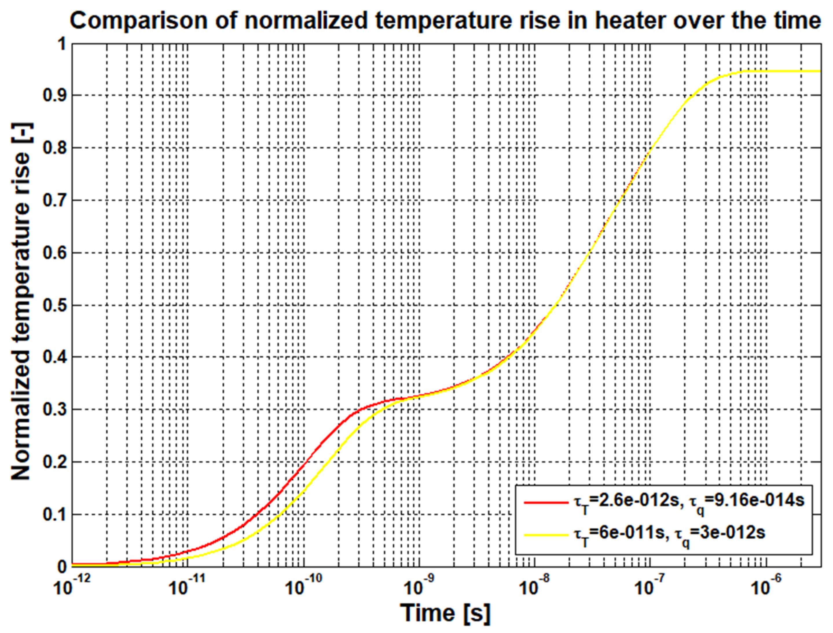
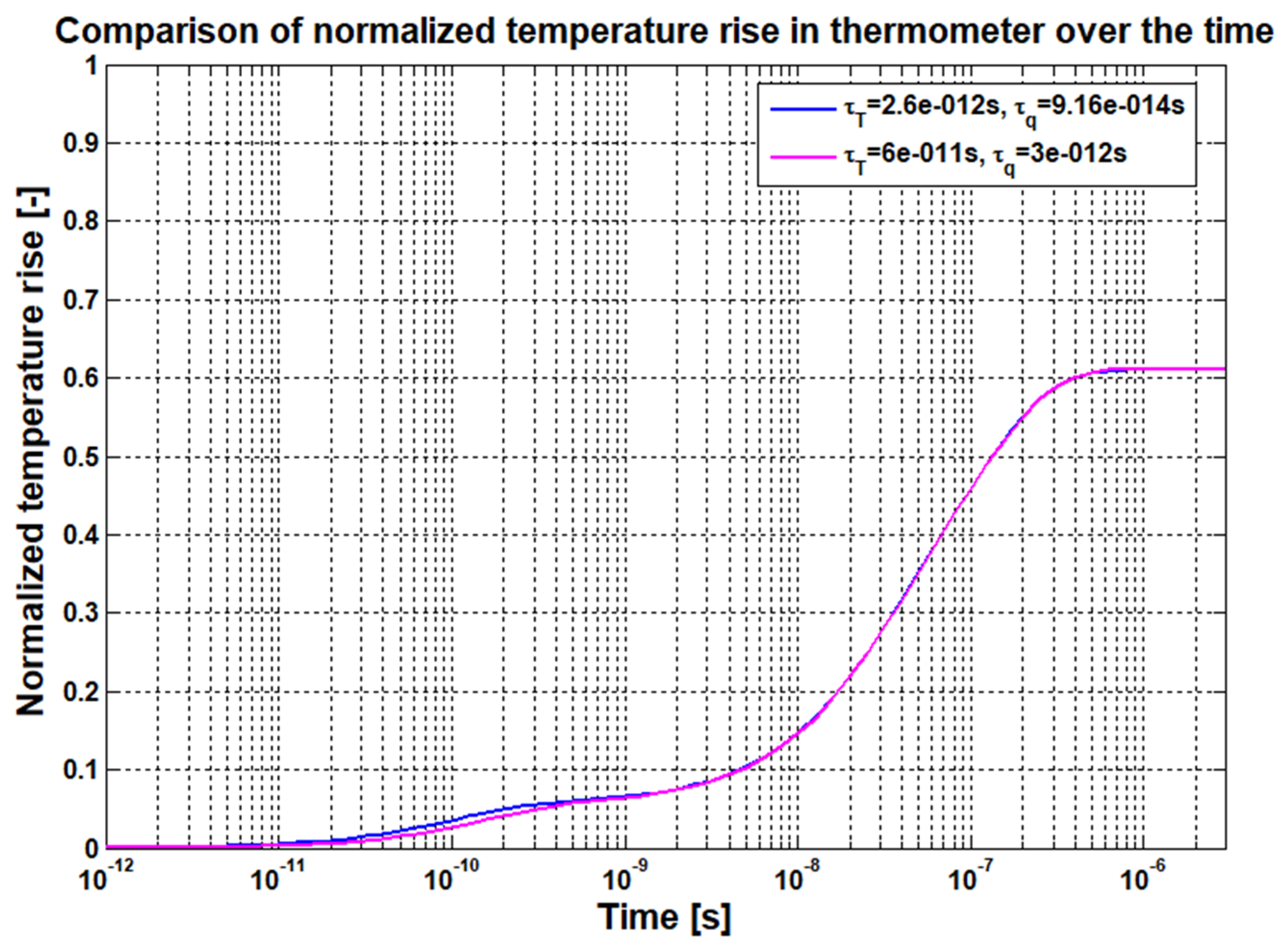
  • τT = 60 ps, τq = 3 ps (all layers)
  • τT = 2.6 ps, τq = 0.0916 ps (platinum resistors) and τT = 60 ps, τq = 3 ps (all remaining layers).
The results, as demonstrated in Figure 3 and Figure 4, were additionally normalized in order to make their analysis easier. The normalization was prepared in the following way:
T k n o r m ( t ) = T k ( t ) max t , k { T k ( t ) }                   k { 1 , 2 , , n x n y } , t R + { 0 }
As it can be seen, the average temperature rise inside the heater is less than 95% of the maximal recorded temperature rise, while the temperature rise in the platinum sensor is characterized by a slightly more than 61% of the highest observed temperature rise. Differences in temperature rise values yielded for analyzed sets of DPL model parameters are observed between 1 ps and 1 ns.
Time shifts between observed lines in Figure 3 and Figure 4 were plotted in Figure 5. In order to show differences between results, excluding and including air conductivity investigation presented in Section 2.4, a time shift analysis over the time, demonstrated in Figure 6, was carried out. In this figure, “new kair” means the thermal conductivity of the air layer between platinum resistors calculated based on the analysis shown in Section 2.4. As a comparison, the simulation results obtained for both DPL time lags equal to zero for the air layer are also included.
Taking into consideration the sensitivity of yielded results to even small changes of the air layer material parameters, in the second part of the simulation, values, calculated considering the investigation described in Section 2.4, were employed only.

3.2. Final Simulation Results and Comparison to Real Measurements of the Test Structure

The analysis in the previous subsections shows that there is a need for calculation of the proper material parameters for the air layer, especially between platinum resistors of the test structure. Moreover, results of further research suggest using the fractional order of the space derivative of the temperature rise function for the investigated region, as well as this one between platinum resistors and the silicon dioxide, according to the theory described in Section 2.4. Taking into consideration these facts, the simulation of the temperature distribution in the cross-sectional area of the real test structure was carried out.
It was assumed that differences between mesh nodes are equal to 10 nm in both axes. Furthermore, values of DPL model time-lag parameters were calculated according to the theory presented in Zubert et al. [8]. Thus, for Platinum resistors, heat-flux time lag was set at approximately 550 ps, while the considered value of the temperature time lag was equal to 15.6 ns. In the case of other materials, investigated parameters were equal to 18 and 480 ns, respectively. Simulation results and their comparison to the real measured data (collected and described in [32,33]) are presented in Figure 7 and Figure 8, for the transient and steady state analyses, respectively. Moreover, in Figure 7, simulation results received by using the classical F–K model are also included, for comparison purposes.
In Figure 7, the results for the heated platinum resistor were marked by dashed and dotted lines, while those ones obtained for the temperature sensor were plotted with dashed lines. Moreover, outputs for the heater and thermometer were marked by the red and blue curves, respectively. On the other hand, measurement data (collected and described in Janicki et al. [32,33]) were plotted, using green lines, while results obtained by using the F–K model were marked by the black color.
The maximal temperature rise above the ambient temperature was observed at the top surface of the heat source, i.e., in the first platinum resistor (layer 3). Its value is nearly 60 K. On the other hand, the temperature rise recorded at the surface of the temperature sensor, i.e., the second platinum resistor (layer 4), is about 6 K, which states approximately 10% of the temperature rise observed in the heat source.
Both of the investigated temperature rises coincide almost exactly with measurements of the real structure (green curves in Figure 7). Parameter αx allows for changing the result curves’ slopes, while DPL model parameters τq and τT cause the curves to shift over the time. The mentioned change is proportional to the parameters’ values.
In order to check the quality of the obtained results for used the discretization mesh and mesh nodes distances (10 nm), which were described in Section 2.2, the simulation curves’ fitting to the measured one was considered. Each curve was plotted based on 703 points logarithmically distributed over the time. Then, such metrics as coefficient of determination (R2), root mean squared error (RMSE), sum of squared estimate error (SSE), and mean squared error (MSE) were calculated. Moreover, to assess the goodness of recognition as a volatility over the time, a Pearson correlation coefficient (corr) was also considered. Determined metrics values are presented in Table 3.
As it can be seen, both the heater and thermometer curves are characterized by relatively small values of MSE, RMSE, and SSE values. Moreover, the coefficient of determination and correlation coefficient suggest a proper recognition of a shape of the measured curve by a simulated one. Generally, it can be stated that calculated metrics (MSE, RMSE, SSE, coefficient of determination, and correlation coefficient) for the simulation fitting to the real data confirm highly accurate simulation results. This situation clearly shows that the proposed approach based on the theory described in Section 2 allows for the production of outputs reflecting the real thermal phenomena observed at the nanoscale. Moreover, as it was shown in Figure 7, the classical F–K model should not be used in the case of electronic nanosized structures.

4. Conclusions

This paper includes the investigation of the heat transfer problems at the nanoscale. A new approach to the heat transfer modeling in modern nanosized structures was considered. It combines the DPL model and the Grünwald–Letnikov fractional derivative. A combination of these mathematical tools allows for the preparation of a complex approach using the Finite Difference Method to temperature distribution determination at the nanoscale, with a high level of accuracy, as is confirmed by the measurement of a real test structure.
An important novelty described in this paper is the use of a DPL model with a fractional order space derivative of a temperature function based on the Grünwald–Letnikov derivative operator. This operator, as well as the proposed time–space discretization schema, is a bridge between experimentally confirmed DPL mesoscopic model with the ballistic heat transport model with dynamic temperature changes’ intensification useful for quasi 1-D nanostructures and for radiative heat transport without phonon collisions. This solution allows for the consideration of such physical behaviors like time needed for a heat flux or temperature gradient changes. Thus, a modeling of a heat diffusion can be investigated by making realistic assumptions, which was not possible in the case of the F–K model use and real relaxation thermal properties of material at mesoscopic scale. The research has shown that the proposed GL DPL model is more realistic than the commonly used Fourier–Kirchhoff model.
The manuscript describes also proposed an approximation scheme of a modern DPL heat transfer model based on the Finite Difference Method approach prepared for the two-dimensional cross-section of the real test nanometric electronic structure manufactured at the Institute of Electron Technology in Warsaw. The investigation has shown that there is a possibility to effectively implement a prepared algorithm that allows for the determination of a temperature distribution inside real nanoscale electronic structures, based on proposed an approximation scheme.
Thermal simulation has provided results which coincide almost exactly with the real measurements. It means that prepared methodology is highly accurate and allows modeling of the heat transfer problems by using a modern approach based on the use of the Dual-Phase-Lag model. The considered thermal model is an appropriate methodology for heat-diffusion modeling, especially at the nanoscale.
In the future, the reduction of the DPL model order reduction methodology will be considered in order to save simulation time, decrease a computational power requirements [47], and make the simulation process more efficient.

Author Contributions

The algorithm for the FDM approximation scheme of DPL model for two-dimensional cross-section of investigated test structure, analysis of the Grünwald–Letnikov temperature derivative of a fractional order and the algorithm calculated its values, numerical simulations and evaluation of their results, and preparation of this manuscript were carried out by T.R. Preparation of the algorithm convergence analysis of numerical simulations, equivalent air conductance investigation, and photon tunneling, as well as the radiative heat transfer calculation, thermodynamic models aspects and time delayed PDEs analysis, were performed by M.Z.; M.Z. also supervised the research and made corrections to the manuscript. All authors have read and agreed to the published version of the manuscript.

Funding

The research presented in this paper was carried out and funded within the Polish National Science Centre project OPUS No. 2016/21/B/ST7/02247.

Acknowledgments

Authors would like to express their special thanks to M. Janicki and J. Topilko sharing papers [32,33].

Conflicts of Interest

The authors declare no conflicts of interest.

Nomenclature

SymbolDescriptionSI Unit
Latin symbols
TTemperature rise distribution in analyzed area in relations to ambient temperatureK
aConstant describing an interaction between gas molecules and solid walls-
bInter-atomic distancem
cpSpecific heat of a material for a constant pressure (cp) J kg K
cvVolumetric heat capacity being a product of a specific heat of a material for a constant pressure (cp) and its density (ρ) J m 3 K
Quotient of Planck constant and the value of 2∙πJ∙s
kMaterial thermal conductivity W m K
kBBoltzmann constant J K
qHeat flux density W m 2
qVVolume density of internally generated heat W m 3
ΔsMesh nodes distancem
tTime variables
xSpace variable
x = { [ x 1 , x 2 , , x n ] T , x R n , n N \ { 1 } x ,           x R
mn
Greek symbols
αxOrder of a fractional Grünwald–Letnikov space derivative-
ΛMolecule’s mean free path lengthm
ρMaterial density kg m 3
τTTemperature time lags
τqHeat flux time lags
Matrix and vectors
1 Vector including only 1 values-
a × bMatrix dimensions; a reflect number of rows, b is the number of columns-
Derivatives
Derivative symbol-
f ˙ First derivative of function f-
f ¨ Second derivative of function f-
G L D 0 , s α Fractional Grünwald–Letnikov derivative of order α around point 0 for s variable-
Mathematical operators
D ( ) Difference operator corresponding to changes for Dt →0-
Multiplication operator-
Nabla operator-
ΔLaplace operator-
GLΔαxFractional order of Laplace operator-
Divergence operator in orthogonal Euclidean space-
Sets’ union operator-
TTransposition operator-
Sets and spaces
{ a 1 , a 2 , a 3 , , a n } Finite set of elements-
( a , b ) Open interval between a and b-
span{a,b}Linear subspace generated by vectors a and b-
Functions
Ensemble average-
α Rounding of α value to the smallest integer number higher or equal to α-
diag(∙)Matrix function creating a diagonal matrix from a vector-
repmat(∙)Matrix function replicating a given vector and composing a matrix of required dimensions-
round(α,k)Rounding of α value to kth digit after decimal point-
max s { f ( s ) } Maximum of the set including f function values-
Γ ( ) Special Gamma function-

References

  1. Fourier, J.-B.J. Théorie Analytique de la Chaleur; Firmin Didot: Paris, France, 1822. [Google Scholar]
  2. Fourier, J.-B.J. The Analytical Theory of Heat; Cambridge University Press: London, UK, 1878. [Google Scholar]
  3. Raszkowski, T.; Samson, A. The Numerical Approaches to Heat Transfer Problem in Modern Electronic Structures. Comput. Sci. 2017, 18, 71–93. [Google Scholar] [CrossRef] [Green Version]
  4. Raszkowski, T.; Zubert, M.; Janicki, M.; Napieralski, A. Numerical solution of 1-D DPL heat transfer equation. In Proceedings of the 22nd International Conference Mixed Design of Integrated Circuits and Systems (MIXDES), Torun, Poland, 25–27 June 2015; pp. 436–439. [Google Scholar]
  5. Zubert, M.; Janicki, M.; Raszkowski, T.; Samson, A.; Nowak, P.S.; Pomorski, K. The Heat Transport in Nanoelectronic Devices and PDEs Translation into Hardware Description Languages. Bulletin de la Société des Sciences et des Lettres de Łódź Série Recherches sur les Déformations 2014, LXIV, 69–80. [Google Scholar]
  6. Nabovati, A.; Sellan, D.P.; Amon, C.H. On the lattice Boltzmann method for phonon transport. J. Comput. Phys. 2011, 230, 5864–5876. [Google Scholar] [CrossRef]
  7. Zubert, M.; Raszkowski, T.; Samson, A.; Janicki, M.; Napieralski, A. The distributed thermal model of fin field effect transistor. Microelectron. Reliab. 2016, 67, 9–14. [Google Scholar] [CrossRef]
  8. Zubert, M.; Raszkowski, T.; Samson, A.; Zając, P. Methodology of determining the applicability range of the DPL model to heat transfer in modern integrated circuits comprised of FinFETs. Microelectron. Reliab. 2018, 91, 139–153. [Google Scholar] [CrossRef]
  9. Tzou, D.Y. Macro-to Microscale Heat Transfer: The Lagging Behavior, 2nd ed.; Willey: Hoboken, NJ, USA, 2015. [Google Scholar]
  10. Jou, D.; Casas-Vázquez, J.; Lebon, G. Extended Irreversible Thermodynamics. Rep. Prog. Phys. 1988, 51, 1105–1179. [Google Scholar] [CrossRef] [Green Version]
  11. Jou, D.; Casas-Vázquez, J.; Lebon, G. Extended Irreversible Thermodynamics, 4th ed.; Springer: Berlin/Heidelberg, Germany, 2009. [Google Scholar]
  12. Tzou, D.Y. An Engineering Assessment to the Relaxation Time in Thermal Waves. Int. J. Heat Mass Transf. 1993, 36, 1845–1851. [Google Scholar] [CrossRef]
  13. Tzou, D.Y. A Unified Field Approach for Heat Conduction from Macro- to Micro-Scales. J. Heat Transf. 1995, 117, 8–16. [Google Scholar] [CrossRef]
  14. Grmela, M.; Öttinger, H.C. Dynamics and thermodynamics of complex fluids. I. Development of a general formalism. Phys. Rev. E 1997, 56, 6620–6632. [Google Scholar] [CrossRef]
  15. Öttinger, H.C.; Grmela, M. Dynamics and thermodynamics of complex fluids. II. Illustrations of a general formalism. Phys. Rev. E 1997, 56, 6633–6655. [Google Scholar] [CrossRef]
  16. Pavelka, M.; Klika, V.; Grmela, M. Multiscale Thermo-Dynamics Introduction to GENERIC; de Gruyter: Berlin, Germany, 2018. [Google Scholar] [CrossRef]
  17. Anufriev, R.; Gluchko, S.; Volz, S.; Nomura, M. Quasi-Ballistic Heat Conduction due to Lévy Phonon Flights in Silicon Nanowires. ACS Nano 2018. [Google Scholar] [CrossRef] [PubMed] [Green Version]
  18. Kröger, M.; Hütter, M. Automated symbolic calculations in nonequilibrium thermodynamics. Comput. Phys. Commun. 2010, 181, 2149–2157. [Google Scholar] [CrossRef]
  19. Zhukovsky, K. Exact Negative Solutions for Guyer–Krumhansl Type Equation and the Maximum Principle Violation. Entropy 2017, 19, 440. [Google Scholar] [CrossRef] [Green Version]
  20. Van, P.; Berezovski, A.; Fülöp, T.; Gróf, G.; Kovács, R.; Lovas, Á.; Verhás, J. Guyer-Krumhansl-type heat conduction at room temperature. EPL (Europhys. Lett.) 2017, 118. [Google Scholar] [CrossRef] [Green Version]
  21. Pop, E.; Sinha, S.; Goodson, K.E. Heat Generation and Transport in Nanometer-Scale Transistors. Proc. IEEE 2006, 94, 1587–1601. [Google Scholar] [CrossRef]
  22. Podlubny, I. Geometric and Physical Interpretation of Fractional Integration and Fractional Differentiation. arXiv 2001. arXiv:math/0110241v1. [Google Scholar]
  23. Li, C.P.; Deng, W. Remarks on fractional derivatives. Appl. Math. Comput. 2007, 187. [Google Scholar] [CrossRef]
  24. Li, C.P.; Qian, D.L.; Chen, Y.Q. On Riemann-Liouville and Caputo Derivatives. Discret. Dyn. Nat. Soc. 2011, 2011, 562494. [Google Scholar] [CrossRef] [Green Version]
  25. Li, C.P.; Zhao, Z.G. Introduction to fractional integrability and differentiability. Eur. Phys. J. Spec. Top. 2011, 193, 5–26. [Google Scholar] [CrossRef]
  26. Cattaneo, M.C. A form of heat conduction equation which eliminates the paradox of instantaneous propagation. C.R. Acad. Sci. I Math. 1958, 247, 431–433. [Google Scholar]
  27. Cattaneo, C. Sur une forme de l’equation de la chaleur eliminant le paradoxe d’une propagation instantanee (in French). Comptes Rendus de l’Académie des Sciences 1958, 247, 431–433. [Google Scholar]
  28. Vernotte, P. Les paradoxes de la theorie continue de l’equation de la chaleur (in French). C. R. Acad. Sci. 1958, 246, 3154–3155. [Google Scholar]
  29. Vermeersch, B.; De Mey, G. Non-Fourier thermal conduction in nano-scaled electronic structures. Analog Integr. Circ. Signal Process. 2008, 55, 197–204. [Google Scholar] [CrossRef]
  30. Kovács, R.; Ván, P. Generalized heat conduction in heat pulse experiments. Int. J. Heat Mass Transf. 2015, 83, 613–620. [Google Scholar] [CrossRef] [Green Version]
  31. Raszkowski, T.; Samson, A.; Zubert, M. Temperature Distribution Changes Analysis Based on Grünwald-Letnikov Space Derivative. Bull. Soc. Sci. Lettres Łódź 2018, LXVIII, 141–152. [Google Scholar]
  32. Sobczak, A.; Topilko, J.; Zajac, P.; Pietrzak, P.; Janicki, M. Compact Thermal Modelling of Nanostructures Containing Thin Film Platinum Resistors. In Proceedings of the 21st International Conference on Thermal, Mechanical and Multi-Physics Simulation and Experiments in Microelectronics and Microsystems (EuroSimE), 6–27 July 2020. in press. [Google Scholar]
  33. Janicki, M.; Topilko, J.; Sobczak, A.; Zajac, P.; Pietrzak, P.; Napieralski, A. Measurement and Simulation of Test Structures Dedicated to the Investigation of Heat Diffusion at Nanoscale. In Proceedings of the 20th International Conference on Thermal, Mechanical and Multi-Physics Simulation and Experiments in Microelectronics and Microsystems (EuroSimE), Hannover, Germany, 24–27 March 2019. [Google Scholar] [CrossRef]
  34. Raszkowski, T.; Samson, A.; Zubert, M. Investigation of Heat Distribution using Non-integer Order Time Derivative. Bull. Soc. Sci. Lettres Łódź Série Rech. Déformations 2018, LXVIII, 79–92. [Google Scholar]
  35. Curtiss, C.F.; Hirschfelder, J.O. Integration of stiff equations. Proc. Natl. Acad. Sci. USA 1952, 38, 235–243. [Google Scholar] [CrossRef] [Green Version]
  36. Ascher, U.M.; Petzold, L.R. Computer Methods for Ordinary Differential-Algebraic Equations; SIAM: Philadelphia, PA, USA, 1998. [Google Scholar]
  37. Süli, E.; Mayers, D. An Introduction to Numerical Analysis; Cambridge University Press: Cambridge, UK, 2003. [Google Scholar]
  38. Auzinger, W.; Herfort, W.N. A uniform quantitative stiff stability estimate for BDF schemes. Opusc. Math. 2006, 26, 203–227. [Google Scholar]
  39. Raszkowski, T.; Samson, A.; Zubert, M. Dual-Phase-Lag Model Order Reduction Using Krylov Subspace Method for 2-Dimensional Structures. Bull. Soc. Sci. Lettres Łódź Série Rech. Déformations 2018, LXVIII, 55–68. [Google Scholar]
  40. Raszkowski, T.; Samson, A.; Zubert, M.; Janicki, M.; Napieralski, A. The numerical analysis of heat transfer at nanoscale using full and reduced DPL models. In Proceedings of the International Conference on Thermal, Mechanical and Multi-Physics Simulation and Experiments in Microelectronics and Microsystems (EuroSimE), Dresden, Germany, 3–5 April 2017. [Google Scholar]
  41. Bahrami, M.; Yanavovich, M.M.; Culham, J.R.; Thermophys, J. Thermal joint resistance of conforming rough surfaces with gas-filled gaps. AIAA J. Thermophys. Heat Transf. 2004, 18, 318–325. [Google Scholar] [CrossRef]
  42. Bahrami, M.; Culham, J.R.; Yanavovich, M.M.; Schneider, G.E. Review of thermal joint resistance models for non-conforming rough surfaces. AMSE J. Appl. Mech. Rev. 2006, 59, 1–12. [Google Scholar] [CrossRef] [Green Version]
  43. Volokitin, A.I.; Persson, B.N.J. Radiative heat transfer between nanostructures. Phys. Rev. B 2001, 63, 205404. [Google Scholar] [CrossRef] [Green Version]
  44. Volokitin, A.I.; Persson, B.N.J. Resonant photon tunneling enhancement of the radiative heat transfer. Phys. Rev. B 2004, 69, 045417. [Google Scholar] [CrossRef] [Green Version]
  45. Raszkowski, T. Numerical Modelling of Thermal Phenomena in Nanometric Semiconductor Structures. Ph.D. Dissertation, Lodz University of Technology, Lodz, Poland, 2019. (In Polish). [Google Scholar]
  46. Incropera, F.P.; DeWitt, D.P.; Bergman, T.L.; Lavine, A.S. Fundamentals of Heat and Mass Transfer, 6th ed.; John Wiley & Sons Inc.: Hoboken, NJ, USA, 2007. [Google Scholar]
  47. Górecki, K.; Górecki, P. Compact electrothermal model of laboratory made GaN Schottky diodes. Microelectron. Int. 2020, Paper version in press 3/2020. [Google Scholar] [CrossRef]
Figure 1. Geometry of cross-sectional area of the investigated test structure.
Energies 13 02379 g001
Figure 2. The graphical representation of discretization mesh and nodes’ numbering. Reprint with permission [34,39]; Copyright 2018, ŁTN.
Energies 13 02379 g002
Figure 3. Average temperature rises over the time inside heat source (excluding investigation in Section 2.4).
Energies 13 02379 g003
Figure 4. Average temperature rises over the time inside temperature sensor (excluding investigation in Section 2.4).
Energies 13 02379 g004
Figure 5. Time shifts over the time for temperature rises in heat source and temperature sensor (excluding investigation in Section 2.4).
Energies 13 02379 g005
Figure 6. Time shifts over the time for temperature rises observed in the heat source and temperature sensor (including analysis in Section 2.4).
Energies 13 02379 g006
Figure 7. Comparison of normalized temperature rises in heater and thermometer.
Energies 13 02379 g007
Figure 8. Steady-state temperature distribution in cross-sectional area of investigated structure.
Energies 13 02379 g008
Table 1. Selected Heat Transfer Model transformed into time delayed Partial Differential Equation.
Heat Transfer ModelDerived Time Delayed PDE
(a)
DPL equation [12,13] for τT > τq > 0,
Maxwell–Cattaneo–Vernotte equation [26,27,28] for τq > 0, τT = 0 (more details in Vermeersch and De Mey as well as Kovács and Ván papers [29,30]), and F–K Equations (1)–(2) for τq = τT = 0:
{ c v T ( x , t ) t = q ( x , t ) q ( x , t ) + τ q q ( x , t ) t = k T ( x , t ) k τ T T ( x , t ) t
c v T ( x , t + τ q ) t = k Δ T ( x , t + τ T )

c v T ( x , t + τ q τ T ) t = k Δ T ( x , t )
(b)
Ballistic-conductive heat transfer model for τq > 0, τQ > 0, k12k12 ≤ 0 (more details [30])
{ c v T ( x , t ) t = q ( x , t ) τ q q ( x , t ) t + q ( x , t ) = k T ( x , t ) k 21 Q ( x , t ) τ Q Q ( x , t ) t + Q ( x , t ) = k 12 q ( x , t )

c v T ( x , t + τ q ) t = = k Δ T ( x , t ) c v k 12 k 21 Δ T ( x , t τ Q ) t
(c)
Proposed DPL model [12,13], with fractional order of the temperature function space derivative based on Grünwald–Letnikov theory for τq > 0, τT > 0, 2 < αx < 2.5 (more details in [31]):
c v T ( x , t ) t + τ q c v 2 T ( x , t ) t 2 = = k G L Δ α x T ( x , t ) + k τ T G L Δ α x T ( x , t ) t
c v T ( x , t + τ q ) t = k G L Δ α x T ( x , t + τ T )

c v T ( x , t + τ q τ T ) t = k G L Δ α x T ( x , t )
Table 2. Considered material parameters’ values [46].
LayerMaterial k [ W m K ]   ρ [ kg m 3 ]   c p [ J kg K ]  
1 (wafer)Silicon (Si)1482330712
2 (oxide)Silicon dioxide (SiO2)1.382220745
3 (heater)Platinum (Pt)71.621,450133
4 (thermometer)Platinum (Pt)71.621,450133
5 (ambient)Air0.0263 *1.16141.007
Table 3. Evaluation of goodness of fitting of simulation results to real data.
Temperature Distribution SimulationMSERMSESSER2Corr
Heater8.5837∙10−40.02930.60340.95720.9973
Thermometer9.5540∙10−50.00980.04720.95540.9748

