Regional Study of Changes in Wind Power in the Indian Shelf Seas over the Last 40 Years

Abstract

Wind power variations at two heights (the surface level and turbine hub level) were investigated at 20 locations in the shelf seas of India using hourly fifth generation European Centre for Medium-Range Weather Forecasts (ECMWF) atmospheric reanalyses of the global climate (ERA5) data covering the last 40 years (1979 to 2018). The interannual and seasonal variability in wind power was studied. The wind power density, the exceedance probability of power density and the exploitable wind resources were examined. In the Indian shelf seas, the annual mean wind power density at 10 m above mean sea level varies from 82 to 353 W/m². Wind power density at 110.8 m is 20% to 40% higher than at 10 m above mean sea level. The study shows that the shelf seas have an abundance of wind power, with wind speeds over 3 m/s during 90% of the time at locations 1 to 3, 12 and 13, with a high occurrence of exploitable wind energy above 0.7 × 10³ kWh/m². Among the locations studied, the most power-rich area was location 12, where during ~62% of the time power was greater than 200 W/m². A significant change (~10–35%) in inter-annual wind power density was detected at a few locations, and these variations were associated with Indian summer monsoon and El Niño–Southern Oscillation events. Trend analysis suggests a decreasing trend in the annual mean wind power density for most of the locations in the Indian shelf seas over the last 40 years. Wind power has considerable directional distribution, and at different locations the annual wind power from the dominant direction is 10% to 79% of the total available power from all directions.

1. Introduction

Energy is a significant factor for sectoral development and the improvement of quality of life. Among the renewable sources of energy, wind is one of the largest emerging sources of energy, along with solar energy [1]. Worldwide the progress of wind energy projects has been relatively strong over the last few years due to the increased price of oil, limited availability of fossil fuel, and environmental pollution [2]. Globally, around 52 GW of wind power was added in 2017, resulting in the capacity of wind power generation rising to 540 GW [3] and by 2020, it is expected to exceed 760 GW [4]. Already in some countries a significant share of power generation is from wind; e.g., Demark (42%), Germany (13.3%), Ireland (23%), Portugal (23.2%), Spain (18%), and United Kingdom (11%) [5]. By 2050, wind energy resources will contribute ~41% of global installed electricity generation [3].

Based on the analysis of wind data from satellite, wind resource assessments have been made for the US Atlantic coast [6], Europe [7], South China Sea [8], and many other regions [9]. A global wind energy resource assessment was performed by Zheng et al. [10]. A comprehensive review of wind resource assessment all over the world was carried out by Murthy and Rahi [11]. The Gujarat Energy and Research Management Institute, Gandhinagar has carried out studies on wind power resources and prepared a map for all the states of India [12]. Using cross-calibrated, multi-platform wind data, Zheng et al. [13] examined the wind energy density in the global ocean and observed that affluent areas in the ocean are located in the west belts of the Northern Hemisphere (500–1000 W/m²) and the Southern Hemisphere (800–1600 W/m²). Olauson [14] reported the wind power of various countries and regions using fifth generation European Centre for Medium-Range Weather Forecasts (ECMWF) atmospheric reanalyses of the global climate (ERA5) data [15]. The study based on the global wind speeds from the Modern-Era Retrospective Analysis for Research and Applications-2 (MERRA2) reanalysis data set produced by National Aeronautics and Space Administration’s (NASA) Global Modeling and Assimilation Office (GMAO) indicates that the estimates of the global wind energy potential vary across a wide range [16].

Wind speed at an onshore location is influenced by higher surface roughness due to the elevation, terrain, and buildings, as well as air density, apart from other weather influences. In contrast, in offshore locations [17], the wind speed in areas that are not close to the land is not subject to these factors which influence the changes in wind speed onshore. Hence, offshore resources are higher and more homogenous over larger areas. Since the population is heavily concentrated in coastal areas, the demand for electricity is also higher in coastal areas. So far, 90% of wind farms are located on the land. The size of wind farms in offshore locations increased from 80 MW to 561 MW from 2007 to 2018 [18]. In 2018, the capacity of offshore wind farms installed in the world’s oceans was 23.1 GW, and they are mostly off the coasts of the UK (34%), Germany (28%), and China (20%) [19]. India is yet to install an offshore wind turbine, and only a LIght Detection And Ranging (LIDAR) capable of measuring winds near the hub height of a wind turbine is installed off Pipavav (~23 km from the coast). Even though the shelf seas contain much richer wind energy resources than the land [1,13], studies in the Indian shelf seas are limited. Using Oceansat-2 Scatterometer, a study on offshore wind resource assessment was done in the state of Karnataka by Sanjeev and Chandra [20].

Although wind power is a clean energy source, wind power is characterized by fluctuations due to the non-stationary nature of wind speed [21]. Hence, wind farm output is significantly influenced by wind speed, and it is essential to identify the locations with high and steady wind speed. For making policy decisions related to selecting the wind farm site, apart from average annual power, variations in wind power at different time scales, such as monthly, seasonal, and inter-annual, are required. From sea level, 80 to 120 m is the height at which modern wind turbines are placed [5]. Generally, the wind speed data from satellite altimetry and weather stations are for the height of 10 m above the ocean surface, and several statistical methods are used to derive wind speed at the turbine height. Therefore, for wind farm planning, there is a need to get wind power data for different levels above the ocean surface, where the wind turbines operate. Depending on the consistency of the wind resources at a location, the power from wind turbines vary. The long-term variations of the wind power in the Indian shelf seas are not yet known.

Motivated by these factors, the objective of the present study was to quantify the wind power resources in the Indian shelf seas (Figure 1) at surface and wind turbine hub height (110.8 m), and changes (seasonal, intra-annual and inter-annual) during the last 40 years. The study also examined the high wind power episodes that impact wind turbines and the factor responsible for these episodes. Forty years of data, which is higher than the minimum (~30 years) period recommended by the World Meteorological Organization to make reliable estimations of climate variables in a region, were used to examine the long-term variations of the wind power and its linkage to the interannual modes of climate variability.

The remainder of the paper is organized as follows. The data used in the study and the methodology is described in Section 2. Section 3 describes the variations in wind power and its consistency, availability of exploitable wind speed at different locations, directional distribution of wind power, long-term changes in wind power, and its association with El Niño–Southern Oscillation (ENSO). Finally, conclusions are provided in Section 4.

2. Data and Methodology

2.1. Data

Wind data at 10 m (usually referred to as surface winds) and 110.8 m (1000 hPa, referred to as hub height winds) above mean sea level were obtained from ERA5 atmospheric reanalyses of the global climate produced by the ECMWF [15]. The advantage of reanalysis data is that these are often freely and globally available and have good spatial and temporal coverage. Zonal (u) and meridional wind (v) data were downloaded for 20 locations in the Indian shelf seas for the period from 1 January 1979 to 31 December 2018 at 1-h intervals for use in the study. Locations in the Indian shelf seas spaced ~1.5° latitude were selected for the study and are indicated in Figure 1. The ERA5 assimilation system used the most up-to-date version of the Integrated Forecasting System (IFS Cycle 41r2) and current parameterization technique of the earth process, which allows use of a variational bias scheme for not only satellite observation, but also for aircraft, ozone, and surface pressure data. In ERA5, hourly data is available at a 31 km (~0.28°) horizontal resolution, with 37 vertical levels up to 1 hPa. ERA5 does not capture variability at a smaller temporal resolution, since the data is at an hourly interval. The water depth of the grid point varies from 27 to 129 m, whereas the water depth in the grid has large variations (

Table 1. Wind power resource in different locations.

Location	Geographic Position	Water Depth (m)		Annual Mean Wind Power Density (W/m2)		Occurrence of Exploitable Wind Energy (%)
						>50 W/m2		>200 W/m2
		Range in Block	at Grid Point	10 m	110.8 m	10 m	110.8 m	10 m	110.8 m
1	22.50° N; 68.25° E	36–89	63	200.33	254.26	78	83	33	45
2	21.00° N; 69.50° E	44–89	65	203.42	260.30	80	84	33	46
3	19.50° N; 71.25° E	45–86	75	199.25	266.06	75	80	32	43
4	18.00° N; 72.00° E	29–112	47	181.62	237.37	70	74	29	37
5	16.50° N; 72.75° E	33–147	68	157.78	207.59	67	70	25	33
6	15.00° N; 73.50° E	44–102	75	128.55	168.34	61	65	20	28
7	13.50° N; 73.50° E	38–1171	80	131.12	172.81	58	62	21	27
8	12.00° N; 74.50° E	66–1086	129	82.29	108.52	46	51	10	16
9	10.50° N; 75.50° E	42–1171	46	81.86	111.01	49	55	10	18
10	09.00° N; 76.00° E	13–362	90	86.10	117.34	47	51	13	21
11	07.75° N; 77.25° E	47–90	61	299.02	443.64	80	81	58	64
12	08.25° N; 78.25° E	5–1041	28	352.51	446.33	82	84	61	67
13	10.50° N; 80.25° E	19–261	104	203.33	311.73	80	84	39	52
14	12.00° N; 80.00° E	0–1187	27	107.32	174.00	66	76	15	32
15	13.50° N; 80.50° E	2–1809	90	125.29	179.26	67	73	20	33
16	15.00° N; 80.25° E	1–280	49	131.66	182.73	68	73	23	34
17	16.75° N; 82.50° E	0–1113	99	150.62	209.72	67	73	26	38
18	18.50° N; 84.50° E	0–813	41	100.11	163.58	54	65	15	30
19	20.00° N; 86.75° E	6–995	58	182.57	227.63	65	69	32	38
20	21.00° N; 89.00° E	30–700	75	165.93	196.96	61	64	27	32

). The water depth of planned wind farm sites is an important consideration because the costs and capabilities of different technologies vary widely with water depth [16]. The wind turbine foundation technology changes with the water depths and is generally monopile for depths up to 35 m, jacket for 35 to 50 m, advanced jacket for 50 to 100 m, and floating structure for depth more than 100 m [6].

To identify the reanalysis data that best represent the wind speed features at wind turbine hub heights, Ramon et al. [22] compared five state-of-the-art global reanalyses (ERA-Interim, ERA5, the Japanese 55-year Reanalysis (JRA55), National Centers for Environmental Prediction (NCEP)- National Center for Atmospheric Research (NCAR) Reanalysis 1 and the Modern-Era Retrospective Analysis for Research and Applications-2 (MERRA2)), with the in situ observations for the period 1980–2017. The comparison shows that the ERA5 surface winds offer the best agreement, correlating and reproducing the observed variability better than a multi-reanalysis mean in 35.1% of the tall tower sites on a daily time-scale [22]. The data used in the study close to the coast can be influenced by the land due to internal boundary layers, coastal air-sea interaction effects, and so on.

From the surface winds, the winds at the desired height are also obtained using wind profile power law as given below;

$$V_Z=V_0{(\frac{h_Z}{h_0})}^{{}^{\alpha }}$$

(1)

where V_Z is the wind speed at desired height h_Z in m/s, V₀ is the wind speed at reference height h₀ in m/s. The exponent α is the wind shear coefficient, which varies depending upon the stability of the atmosphere, air parameters, and the morphology of the territory. For the study area, it can be observed that $\propto$ = 0.04 gives wind speed at 110.8 m from the 10 m ERA5 data (Figure 2). Hence, the average wind speed at 110.8 m is ~10% more than that at 10 m and the correlation coefficient between the wind speed at 10 and 110.8 m is 0.9.

2.2. Methodology

The airflow through a wind turbine generates wind energy by transforming the kinetic energy of the air into electric power. Wind power density reported here is the wind power on a unit section perpendicular to the flow [13]. From the hourly wind data, the wind power density (P), a measure for the energy which is available for conversion in the shelf seas of India, was calculated using the expression below.

$$P=\frac{1}{2}\rho V^3$$

(2)

where ρ is the air density taken as 1.225 kg/m³ and V is the wind speed (m/s). The coefficient of variation C_V in wind power density in different months is calculated as the ratio between the standard deviation and the mean. The smaller C_V shows better consistency [13].

The monthly variability index (M_V) was used to study the inter-annual variations and was calculated using the below expression.

$$M_V=\frac{P_{M1}-P_{M2}}{P_{year}}$$

(3)

where P_M1 is the average power density in the most abundant month, P_M2 is the average power density in the weakest month and P_year is the annual average wind power density. The larger the M_V, the higher the monthly variation of energy and it implies weak consistency [13].

The variability index (S_V) was used to quantify the inter-seasonal variations and was computed using the below expression.

$$S_V=\frac{P_{S1}-P_{S2}}{P_{year}}$$

(4)

where P_S1 the average wind power density in most abundant season, P_S2 is the average wind power density in a poor season, P_year is the annual average wind power density.

The seasonal mean wind power density was calculated over the 40 year period. To study the wind energy resources at a location, the total wind power storage per unit area E_P was calculated using the below expression.

$$E_P=\overline{P}T$$

(5)

where $\overline{P}$ is annual average wind power density, T is the total hours in a year (= 8760 h). Hereafter the wind power mentioned is the wind power density.

The trend in annual mean, 95 percentile and 99 percentile wind power was calculated based on the least-squares linear fit method. The slope of the linear best-fit curve to the data for the 40 year period was estimated. A positive slope indicates a wind power increase, and a negative slope indicates a decrease. To identify the cause of high wind power at the locations, the tropical cyclone data obtained from Official US Navy Website Joint Typhoon Warning Centre (JTWC) was used.

3. Results and Discussion

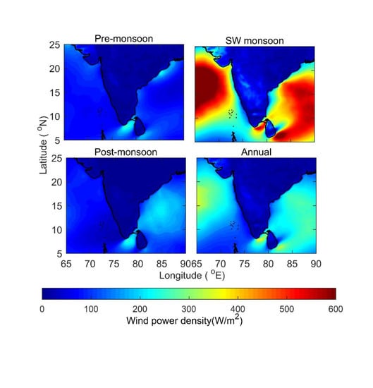
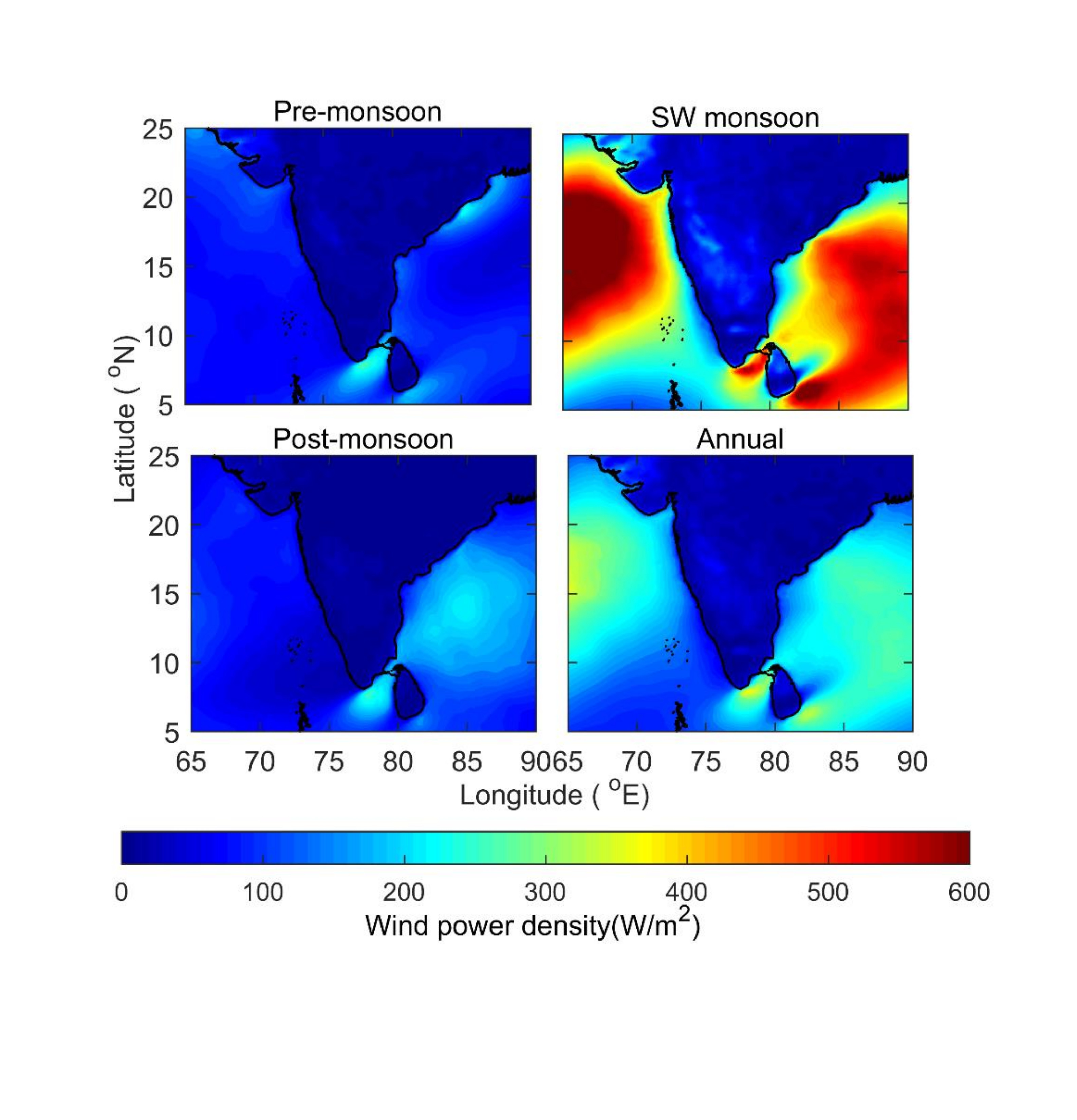
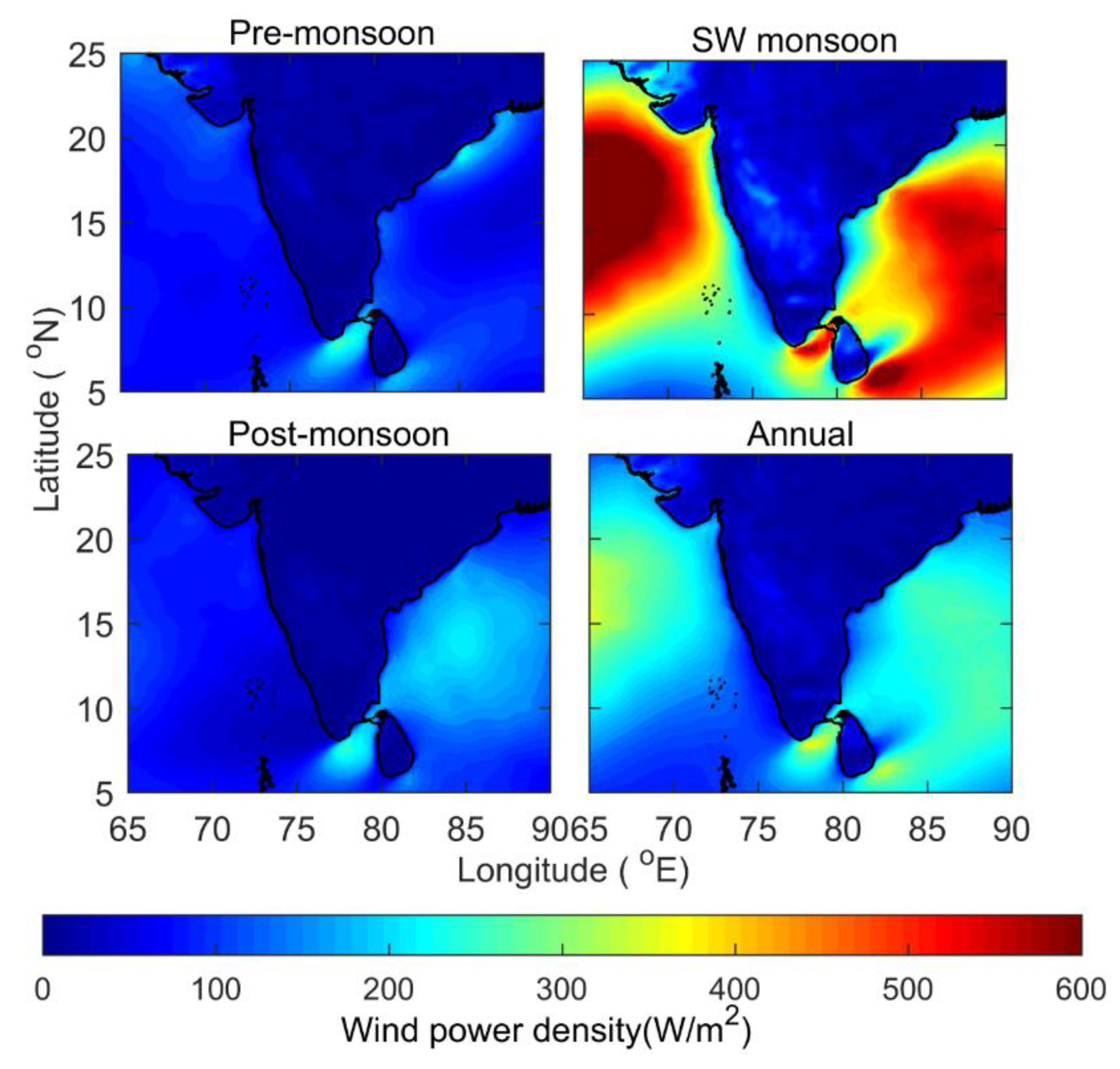
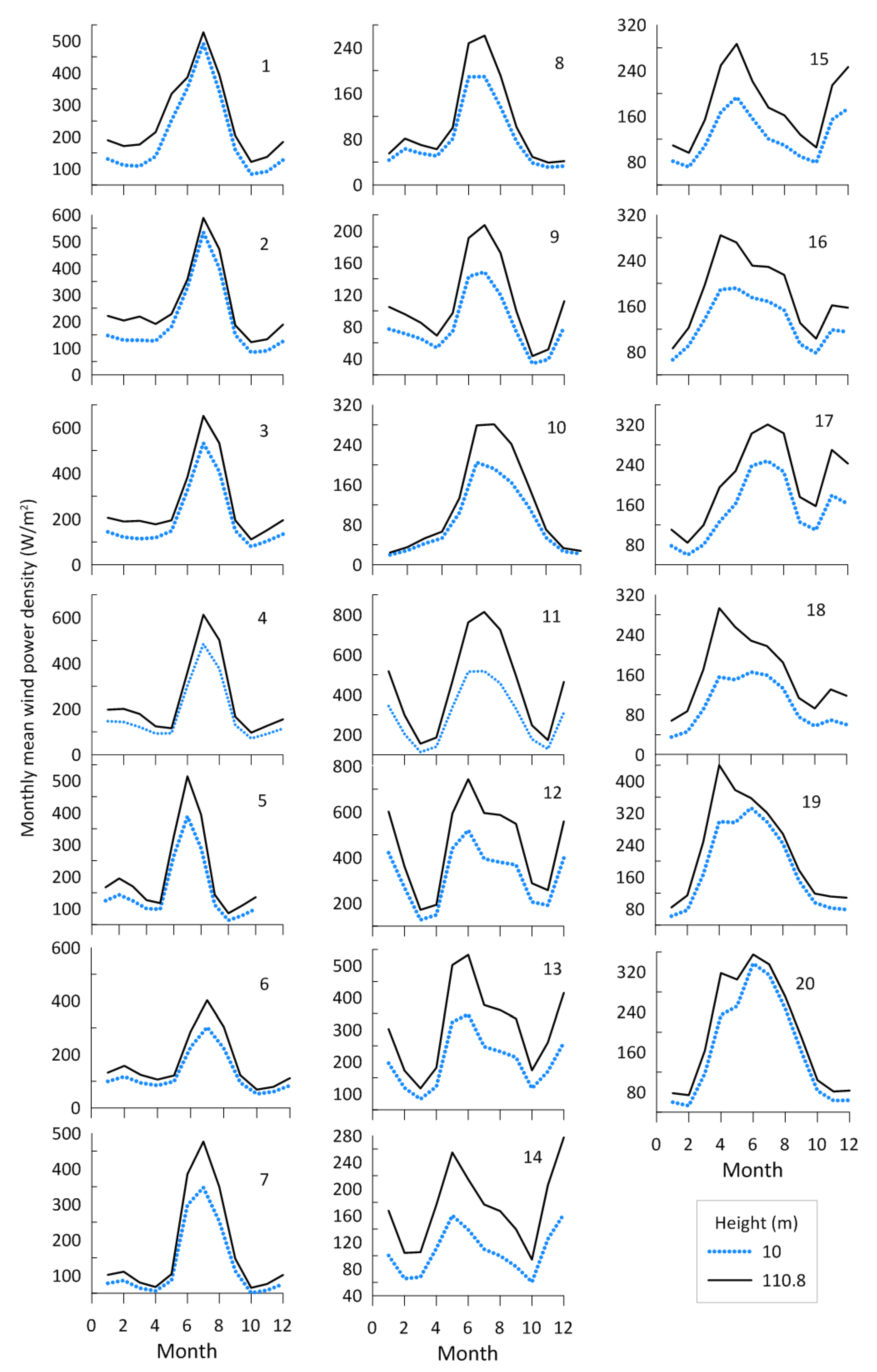
3.1. Variations in Wind Power

The spatial distribution of seasonal average wind power at a height of 10 m above mean sea level over the 40 years is presented in Figure 3 for pre-monsoon (February–May), Indian summer monsoon or southwest (SW) monsoon (June–September), and post-monsoon (October–January) along with annual mean wind power. During the pre and post-monsoon period, the maximum values of wind power were observed in the southern part. In contrast, during the SW monsoon where strong southwest trade winds prevail, the higher wind power is observed at the central Arabian Sea (AS), the region between India and Sri Lanka and the central Bay of Bengal (BoB). Maximum seasonal average wind power during pre-monsoon (277 W/m²) and post-monsoon (260 W/m²) and maximum annual average (369 W/m²) are at 78° E; 8° N (Figure 3).

The seasonal average wind power during the SW monsoon is maximum (876 W/m²) at 65° E; 15.5° N (Figure 3) and is due to the high wind speed in the central west and central AS due to the Findlater jet [23]. Using monthly mean winds, Findlater [23] showed that the low-level jet splits into two branches over the AS, one branch passing southeastward towards Sri Lanka and the other eastward through peninsular India, when active and break monsoons occur at the same time. Hence, during the SW monsoon, wind power is also high at locations off the southern tip of India. Also, throughout the year, wind power is relatively higher in the southern part of India, especially the area between India and Sri Lanka (Figure 3).

Information on the variability of the wind power in monthly and annual scale is required for the selection of a wind power plant. At all the locations in the AS, the maximum level of monthly mean wind power occurs in July, when the intertropical convergence zone is located above the Indian landmass (Figure 4).

At 10 m height, the highest monthly mean wind power among our locations is at location 2 (~534.89 W/m² ), followed by location 3 (~532.60 W/m² ), and occurs in July. Mean wind power during June-August is high at locations 1–7, as the central AS experiences maximum wind power during this period (Figure 3), and it decreases at location 10. The standard deviation of monthly variation is highest at location 11 (~146.76 W/m² at 10 m and 253.34 W/m² at 110.8 m), indicating larger variability as compared to other locations. At all locations, the mean monthly maximum wind power is less than 350 W/m² from December to April. The maximum monthly mean wind power is in different months at different locations in the Bay of Bengal (BoB), i.e., during May, June and July (Figure 4), and it varies from 191.84 W/m² (location 16) to 520.48 W/m² at 10 m above the surface (location 12). At 110.8 m above the surface, the monthly minimum mean wind power varies from 68.01 W/m² (location 18) to 171.65 W/m² (location 12). The maximum wind power at all of the locations other than locations 5, 7, and 9, is during the tropical cyclones (

Table 2. Factor responsible for maximum wind power at 10 m height of different locations.

Location	Maximum Wind Power (W/m2)	Date of Occurrence	Caused by
1	8431.35	20 May 1999	Extremely severe cyclonic storm ARB 01 (02A)
2	8246.88	08 Jun 1998	Extremely Severe Cyclonic Storm ARB 02 (03A)
3	5763.96	18 Jun1996	Severe Cyclonic Storm ARB 01 (04A)
4	5043.88	17 Jun 1996	Severe Cyclonic Storm ARB 01 (04A)
5	3597.72	23 Jul 1989	During SW monsoon
6	3534.93	10 Nov 2009	Cyclonic Storm Phyan
7	3015.67	29 May 2006	During onset of SW monsoon
8	3445.77	07 May 2004	Cyclonic Storm ARB 01
9	2282.54	22 Jun 2007	During SW monsoon
10	2849.04	30 Nov 2017	Very Severe Cyclonic Storm Ockhi
11	2676.34	13 Nov 1992	Severe Cyclonic Storm BOB 07
12	3513.90	13 Nov1992	Severe Cyclonic Storm BOB 07
13	4075.57	03 Dec 1993	Extremely Severe Cyclonic Storm BOB 02
14	4359.53	30 Dec 2011	Very Severe Cyclonic Storm Thane
15	8183.53	12 Dec 2016	Very Severe Cyclonic Storm Vardah
16	10,799.65	12 May 1979	Cyclone One (1B)
17	4414.27	12 Oct 2014	Extremely Severe Cyclonic Storm Hudhud
18	5177.32	12 Oct 2013	Extremely Severe Cyclonic Storm Phailin
19	8239.31	29 Oct 1999	Super Cyclonic Storm BOB 06 (05B)
20	11,081.02	25 May 2009	Severe Cyclonic Storm Aila

). In a nutshell, monthly mean wind power is observed to be at maximum during the SW monsoonal months and annual maximum wind power at all the study locations shows large variations (Figure 5).

The wind power during south-west monsoon is 49–72% of the annual wind power at locations 1 to 11 (Figure 6). During the pre-monsoon period, the wind power is 14–29% of the annual wind power and the highest values are at location 11. During the post-monsoon period, the wind power is 10–27% of the annual wind power; slightly less than that during the pre-monsoon period. Wind power is higher during the pre-monsoon period at the southern locations than at the northern locations. Although the wind power in the south-west monsoon is less at the southern locations (location 11), the highest annual mean wind power in the AS is observed at location 11 (299.02 W/m² at 10 m and 443.64 W/m² at 110.8 m), since the wind power at this location during the pre-monsoon and post-monsoon is high (Figure 7).

For locations in the BoB, the highest seasonal mean wind power is in the south-west monsoon at all locations other than locations 15 and 16 (at 10 m) and location 14 (at 110.8 m) (Figure 7). At locations 15 and 16, the highest seasonal mean wind power is during the pre-monsoon period, whereas at location 14, the highest seasonal mean wind power is in the post-monsoon period. At locations 16 to 20, the lowest seasonal mean wind power is during the post-monsoon period and at other locations, it is in pre-monsoon. In western BoB, the annual mean wind power decreased from south to north and is highest at location 12 (352.51 W/m² at 10 m and 446.33 W/m² at 110.8 m) and lowest at location 18 (100.11 W/m²). Location 12 is located between the Indian landmass and Sri Lankan landmass, and the high wind power in this location is due to the wind channeled by the land topography. During the SW monsoon, the southern branch of the Findlater jet causes high wind speed at this location. This location is also exposed to the northeast monsoon during November–January. Figure 8 shows the time series plot of wind speed at locations 8, 11, and 12 in the year 2018. At location 8, situated in the AS, the wind is high only during the SW monsoon, whereas at locations 11 and 12, the wind speed is high even in the post and pre-monsoon period. Srisha et al. [24] observed that in April and May, the variation in land surface cooling induces a low pressure centered at 11.65° N, 78.16° E in India, and this causes the sudden intensification of winds in the area between India and Sri Lanka. In the northeastern locations (19 and 20), the wind power is higher than those at locations 14 to 18. At location 20, the annual mean wind power is 165.93 W/m² at 10 m height and 196.96 W/m² at 110.8 m height. The inter-annual variation in wind power is 10–35% of the mean annual value at different locations.

Annual mean wind power at 110.8 m is 20% to 60% higher than the wind power at 10 m, and for locations 1 to 8 and 12, it is 30% higher, whereas it is 40 to 60% higher for the remaining locations, except at locations 19 and 20, where it is 20% higher than that at 10 m.

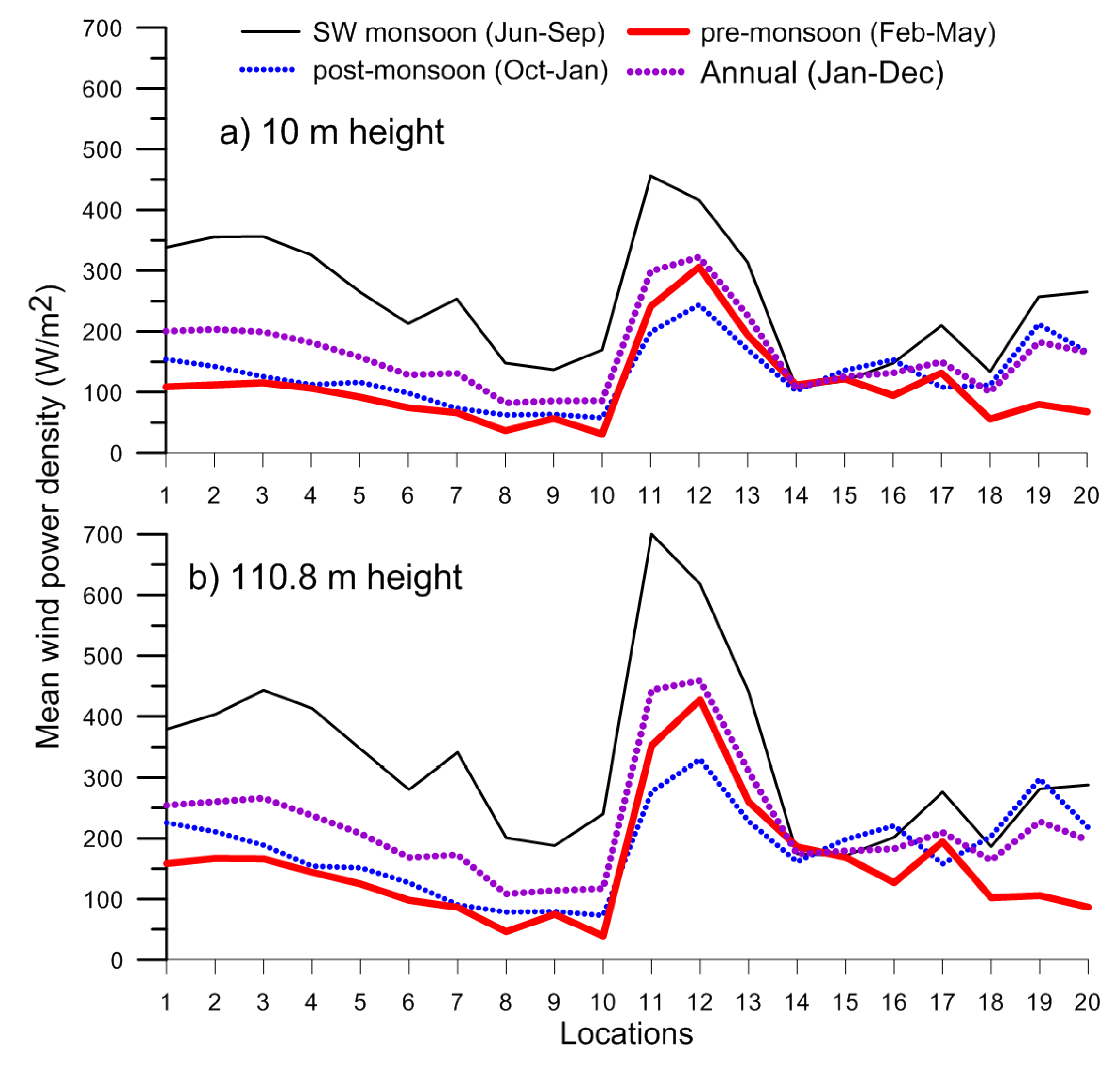
3.2. Characteristics of Wind Power

For the assessment of wind energy resources, the occurrence in the different ranges is an important criterion to measure the degree of energy richness. Usually, the wind power more than 50 W/m² is taken as a power-available area and wind power more than 200 W/m² is a power-rich area [13]. Using hourly wind power from 1 January 1979 to 31 December 2018, the occurrence percentage of wind power more than 50 and 200 W/m² was calculated over 40 years (Table 1). At 10 m, during ~80% of the year, wind power greater than 50 W/m² is found at locations 2 and 11 and at location 12, it is 82%. Wind power greater than 200 W/m² is found at location 12 during 62% of the time. At 110.8 m, high occurrence of wind power greater than 50 W/m² is observed in locations 2, 12, and 13 (84%) followed by location 11 (81%) and wind power greater than 200 W/m² is found in location 12 during 67% of the year.

Wind power shows obvious regional and seasonal differences in Indian shelf regions. During the south-west monsoon, wind power is high at location 11 at both levels; 456.08 W/m² at 10 m and 700.21 W/m² at 110.8 m, whereas location 12 has the highest annual mean power (352.51 and 446.33 W/m² at 10 and 110.8 m). Locations 8 and 9 have the least annual mean wind power (~82 W/m²).

3.3. Consistency of Wind Power

Using hourly wind power from 1 January 1979 to 31 December 2018, the consistency of wind power during the study period is computed for both heights. At 10 m, most of the locations have a minimum C_V in July and it varies within the range of 0.63–0.83. April shows minimum C_V in locations 1, 2, and 15 to 18, and it varies in the range of 0.60–0.78. At 110.8 m, the maximum C_V is in November and December and the range varies from 1.30 to 3.35. Location 10 shows the maximum monthly C_V (3.35) and location 11 shows minimum C_V (0.43). Most of the months show a minimum C_V in July, and it varies within the range of 0.43–0.88.

The monthly averages of wind power from January 1979 to December 2018 were estimated, and the M_V of wind power in Indian shelf regions over the 40 years was examined at both heights. At most of the locations, M_V is below 2 at 10 m and 2.5 at 110.8 m, and is uniform without large regional differences. For both heights, large values of M_V are found in location 7 (2.44 to 2.75) and location 10 (2.14 to 2.18), which means that the monthly consistency of wind power in these locations is poorer than that at other locations.

At 10 and 110.8 m, the wind power S_V in all of the locations is below 1.5 except at location 10 (1.61) and location 18 (1.51), without apparent regional differences. Areas with higher values of wind power S_V are not observed in any of these locations.

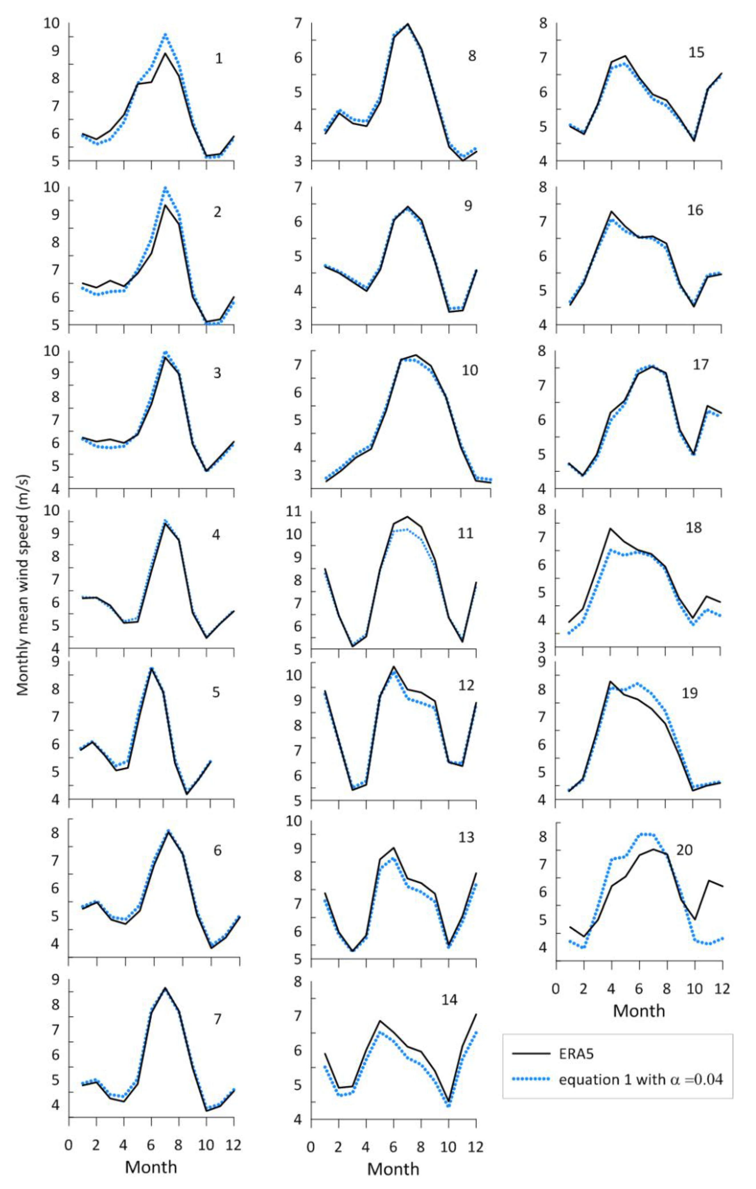
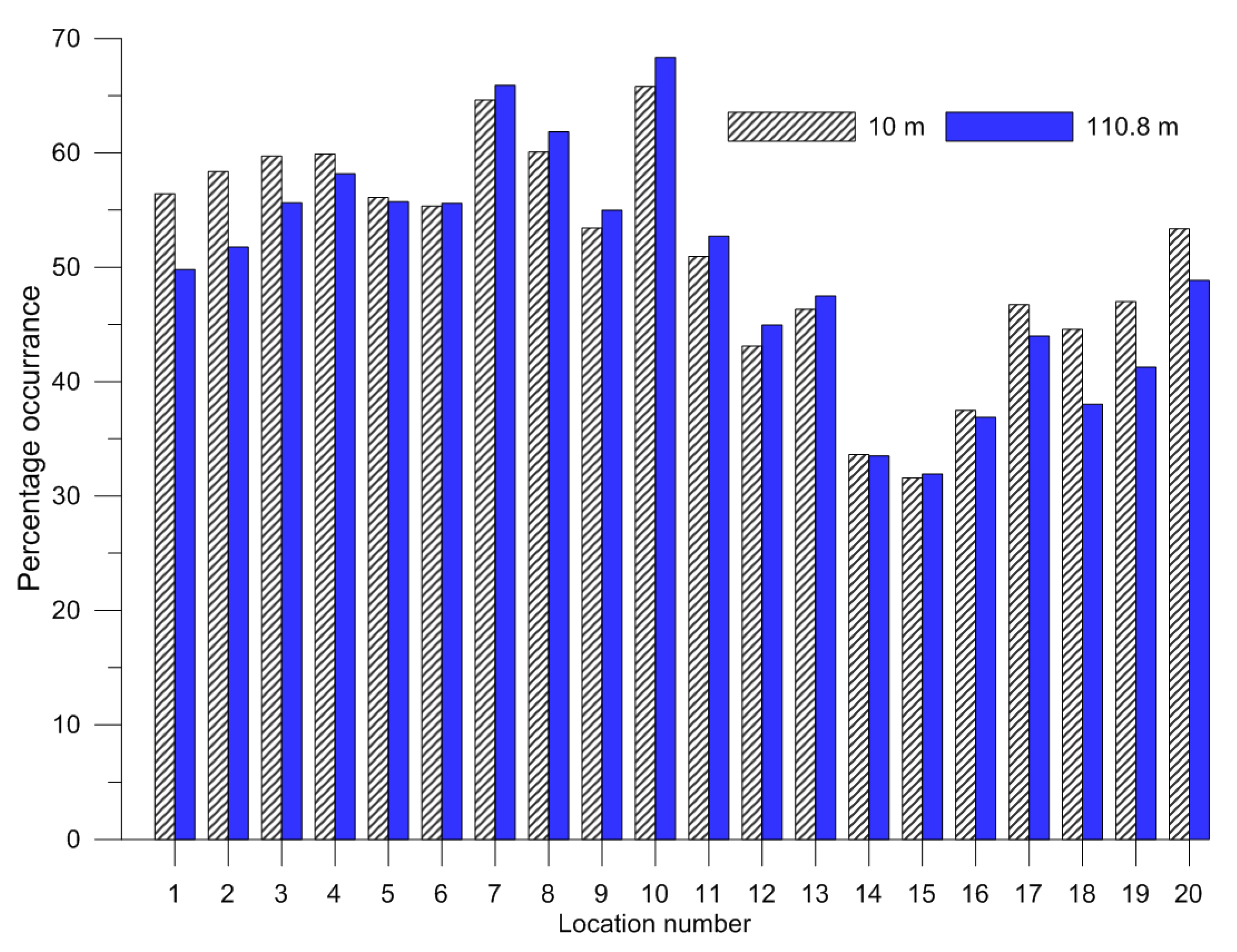
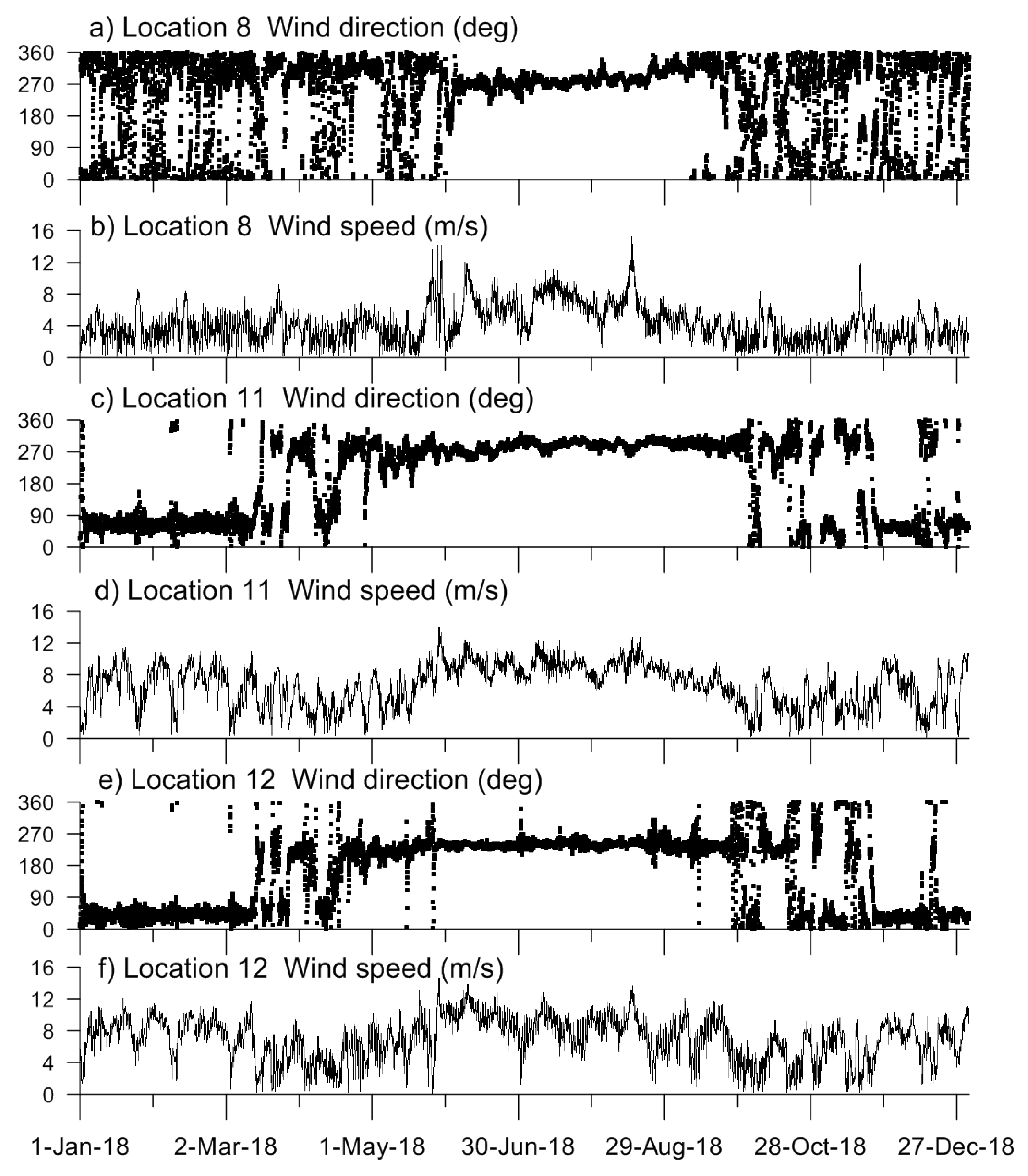
3.4. Exploitable Wind Speed

Generally, 3 m/s is the cut-in speed, i.e., the speed at which the turbines start to produce electricity. The cut-off speed, i.e., the speed at which the turbine shuts down for self-protection, is 25 m/s [13]. Hence, the ideal wind speed in wind power exploitation is 3 to 25 m/s. Over the last 40 years, the percentage occurrence of exploitable wind speed is high at all the locations studied, indicating most times of year are suitable for wind energy resource development (

Table 3. Wind speed occurrence at different heights.

Location	Percentage of Occurrence
	Wind Speed <3 m/s		Wind Speed <4 m/s		Wind Speed >6 m/s		Wind Speed >20 m/s
	10 m	110.8 m	10 m	110.8 m	10 m	110.8 m	10 m	110.8 m
1	7.05	6.09	17.27	13.76	48.12	59.04	0.02	0
2	7.27	5.99	15.93	12.60	49.76	61.17	0	0
3	9.17	7.78	19.95	16.18	45.98	56.56	0	0
4	12.61	11.34	24.60	21.48	41.84	49.85	0	0
5	15.22	13.83	28.02	25.06	38.23	45.72	0	0
6	18.81	17.26	33.50	30.16	32.27	39.45	0	0
7	21.87	19.98	36.95	33.58	31.47	37.74	0	0
8	29.61	26.97	47.62	43.21	19.53	26.26	0	0
9	27.53	24.91	44.82	39.85	20.83	28.82	0	0
10	33.39	31.12	47.89	44.48	23.62	30.87	0	0
11	10.75	10.15	17.66	16.48	66.91	70.58	0	0
12	9.08	8.30	15.01	13.64	70.00	73.81	0	0
13	6.84	5.54	15.87	12.48	54.12	64.85	0	0
14	12.78	9.68	27.25	12.48	29.12	47.44	0	0
15	13.72	11.57	26.95	19.69	35.79	46.92	0	0
16	13.98	11.87	26.93	23.31	37.29	47.40	0	0.01
17	15.10	12.84	27.59	22.53	40.12	50.75	0	0
18	24.62	18.45	40.66	30.50	26.54	41.68	0	0
19	17.62	15.81	29.96	26.77	42.81	48.23	0.08	0.01
20	21.42	19.53	34.73	31.76	38.10	42.79	0.01	0.01

). Along the eastern AS at 10 m, wind speeds greater than 20 m/s only occur at locations 1 and 3 (0.02%). At 110.8 m, wind speeds higher than 20 m/s do not occurr at any locations. In the eastern AS, the highest percentage of wind speeds over 6 m/s occurs at location 11 (66.91% at 10 m and 70.58% at 110.8 m). Among the locations studied, the highest percentage of wind speeds over 6 m/s is at location 12 (70.00% at 10 m and 73.81% at 110.8 m). Along the western BoB at 10 m, wind speeds greater than 20 m/s is occur at locations 19 and 20 (0.28% and 0.01%). At 110.8 m, wind speeds greater than 20 m/s occur at locations 16, 19, and 20 (0.01%).

The 5, 10, 50, 75, 90, and 99 percentile wind speed at two heights for all the locations studied are presented in

Table 4. Different percentile wind speed at 10 and 110.8 m.

Location	Different Percentile Wind Speed (m/s) at 10 m						Different Percentile Wind Speed (m/s) at 110.8 m
	5	10	50	75	90	99	5	10	50	75	90	99
1	2.7	3.4	5.9	7.5	9.2	12.1	2.8	3.6	6.6	8.3	9.9	10.8
2	2.6	3.4	6.0	7.4	9.2	12.2	2.8	3.7	6.6	8.3	9.9	10.9
3	2.4	3.1	5.8	7.4	9.3	12.3	2.5	3.3	6.4	8.3	10.2	11.3
4	2.0	2.7	5.5	7.2	9.0	12.2	2.1	2.8	6.0	7.9	10.0	11.2
5	1.8	2.5	5.3	6.9	8.6	11.6	1.8	2.6	5.7	7.6	9.5	10.7
6	1.6	2.2	4.9	6.5	8.0	10.8	1.6	2.3	5.3	7.1	8.8	9.9
7	1.4	2.0	4.8	6.5	8.2	11.2	1.5	2.1	5.1	7.1	9.1	10.3
8	1.2	1.7	4.1	5.6	6.9	9.7	1.2	1.8	4.4	6.1	7.6	8.6
9	1.2	1.8	4.3	5.8	7.0	9.4	1.3	1.8	4.6	6.3	7.8	8.7
10	1.0	1.5	4.1	5.9	7.2	9.3	1.1	1.5	4.4	6.5	8.0	8.9
11	2.0	2.9	7.5	9.1	10.2	11.9	2.1	3.0	8.4	10.4	11.8	12.5
12	2.2	3.2	7.7	9.3	10.4	11.9	2.3	3.3	8.6	10.5	11.8	12.4
13	2.6	3.3	6.4	8.1	9.5	11.5	2.6	3.5	7.0	9.0	10.6	11.5
14	2.0	2.7	5.1	6.2	7.3	9.0	2.3	3.0	5.9	7.3	8.6	9.4
15	1.9	2.6	5.3	6.6	7.7	9.7	2.1	2.8	5.8	7.4	8.7	9.5
16	1.9	2.6	5.3	6.7	7.9	9.7	2.0	2.8	5.8	7.5	8.9	9.6
17	1.8	2.5	5.4	6.9	8.3	11.0	1.9	2.7	6.1	7.8	9.3	10.2
18	1.3	1.9	4.6	6.1	7.4	9.7	1.5	2.1	5.4	7.2	8.7	9.6
19	1.6	2.3	5.5	7.5	9.1	11.9	1.7	2.4	5.9	8.1	9.8	10.8
20	1.4	2.0	5.1	7.1	8.9	12.1	1.5	2.2	5.8	8.7	11.3	12.9

. The high value of the 5th percentile of the distribution indicates a high consistency of the wind. Table 4 shows that at both the heights, the 5th percentile wind speed is more than 2 m/s at locations 1 to 4 and at 11 to 14. The 10th percentile wind speed is more than 3 m/s at locations 1 to 3, 12, and 13. Among the locations studied, the maximum of the 99 percentile value is 12.3 and 12.5 m/s at hieights of 10 m and 110.8 m respectively (Table 4).

At 10 m, the shelf seas contain rich wind energy and are higher than that over the land. Annually, the total storage of wind energy in most locations is above 0.7 × 10³ kWh/m². The highest values are found in location 12 (~ 3.0 × 10³ kWh/m²) and the lowest values are found in locations 8 to 10 (~ 0.7 × 10³ kWh/m²). At 110.8 m, the total storage of wind energy in most of the locations is above 1.0 × 10³ kWh m⁻² except at locations 8 and 9 (~ 0.9 × 10³ kWh/m²). High-value areas are found in location 12 (~ 3.9 × 10³ kWh/m²) followed by location 11 (~ 3.8 × 10³ kWh/m²).

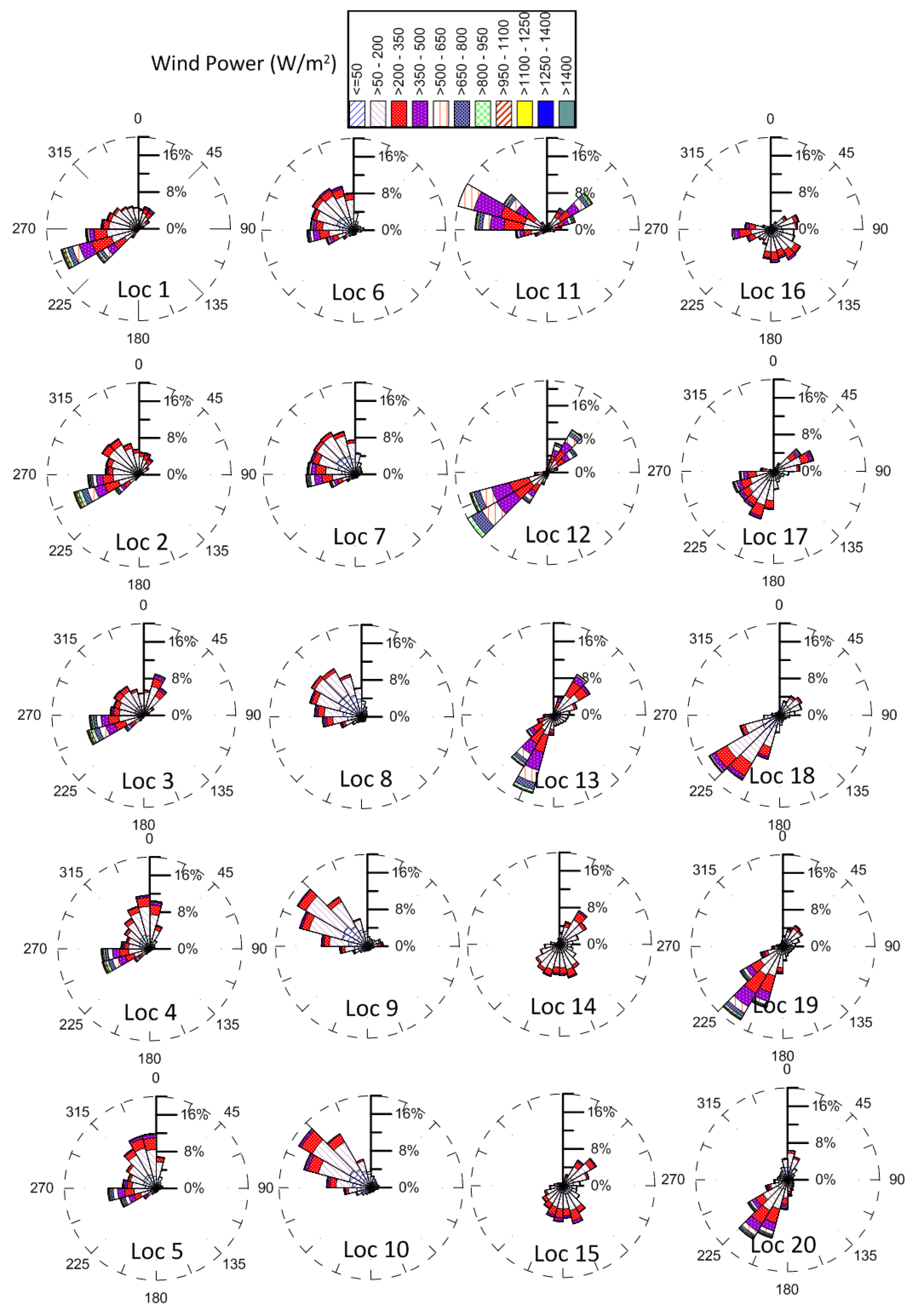
3.5. Directional Distribution of Wind Power

Even though the Yaw drive aligns the wind turbine towards the wind, wind farm configuration depends on the predominant wind direction. Hence, while planning the wind farm layout, information on the direction in which most of the wind energy is available is important [25]. The wind power rose diagrams presented in Figure 9 can be used to determine how to align turbine rows in a wind farm. The wind power rose diagrams indicate that the wind power in the shelf seas is directionally distributed (Figure 9). Winds in the AS are influenced by the Somali jet (which is also known as monsoon low-level-jet or Findlater jet [23]), Shamal winds from the eastern Arabian Peninsula [26], Makran winds from the southern coast of Pakistan [27], and the northeast monsoon winds [28]. Since these wind systems are predominant in the AS, the directional distribution of wind power for most of the locations in the AS are in wide directional sectors (Figure 9). In the BoB, the directional distribution in wind is due to the reversing southwest and northest monsoons and the tropical cyclones. The optimum direction for the wind turbine rotor is 265° to 300° for the AS locations, whereas for locations in the BoB, it is 165° to 235° (

Table 5. Optimum direction for wind turbine and the annual mean wind power component perpendicular to the rotor fan and the corresponding percentage of time in a year at both the levels.

Location	Optimum Direction (Deg)	10 m	110.8 m
		Annual Mean Power (W/m2)	Time (%)	Annual Mean Power (W/m2)	Time (%)
1	265	125.21	78.9	152.01	78.1
2	280	105.80	80.4	127.28	79.7
3	275	109.07	72.0	138.92	71.4
4	290	73.04	74.6	93.30	74.0
5	295	67.41	79.2	87.20	78.8
6	295	67.41	79.2	87.38	79.2
7	295	72.65	79.4	95.41	79.1
8	295	51.41	80.4	68.29	80.5
9	300	56.82	77.5	75.35	77.5
10	300	67.24	79.8	92.40	80.0
11	285	197.10	66.4	293.23	66.6
12	235	201.67	60.8	289.11	60.8
13	210	137.50	50.0	193.54	50.1
14	190	28.04	37.7	46.34	37.9
15	185	34.63	36.2	51.14	35.8
16	165	13.59	24.2	19.59	23.6
17	225	72.62	59.7	98.69	59.6
18	220	71.96	64.6	115.93	65.1
19	215	131.34	60.7	164.96	60.9
20	210	108.04	58.5	128.90	58.3

). For location 12, the optimum direction is 235°. The wind power available in the optimum direction at 10 and 110.8 m height was estimated and is presented in Table 5. At both the heights (10 and 110.8 m), the wind power in the optimum direction is 10% to 79% at different locations (Table 5) compared to the wind power from all directions (Table 1) and the reduction is maximum at locations 14 to 16.

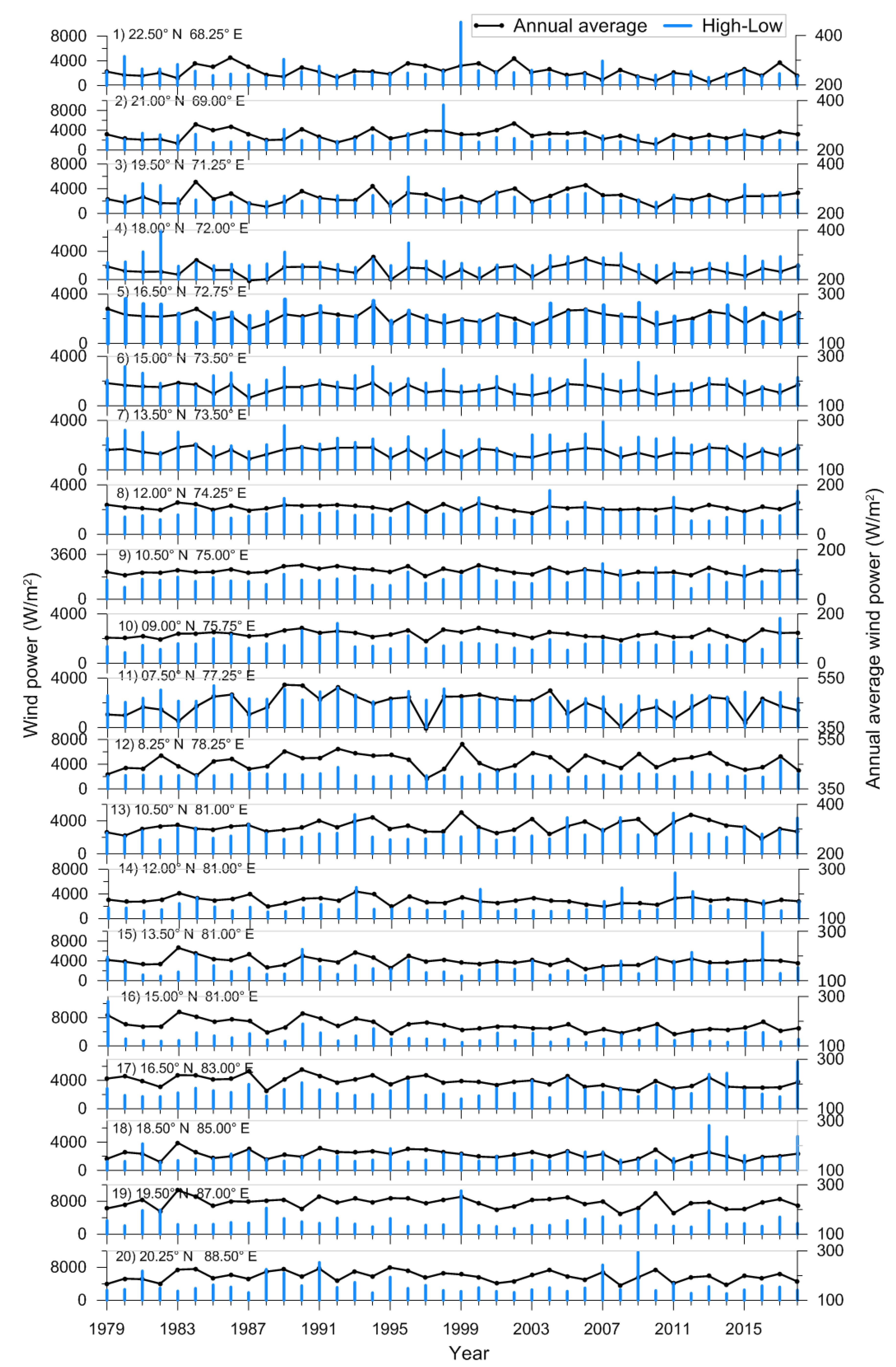
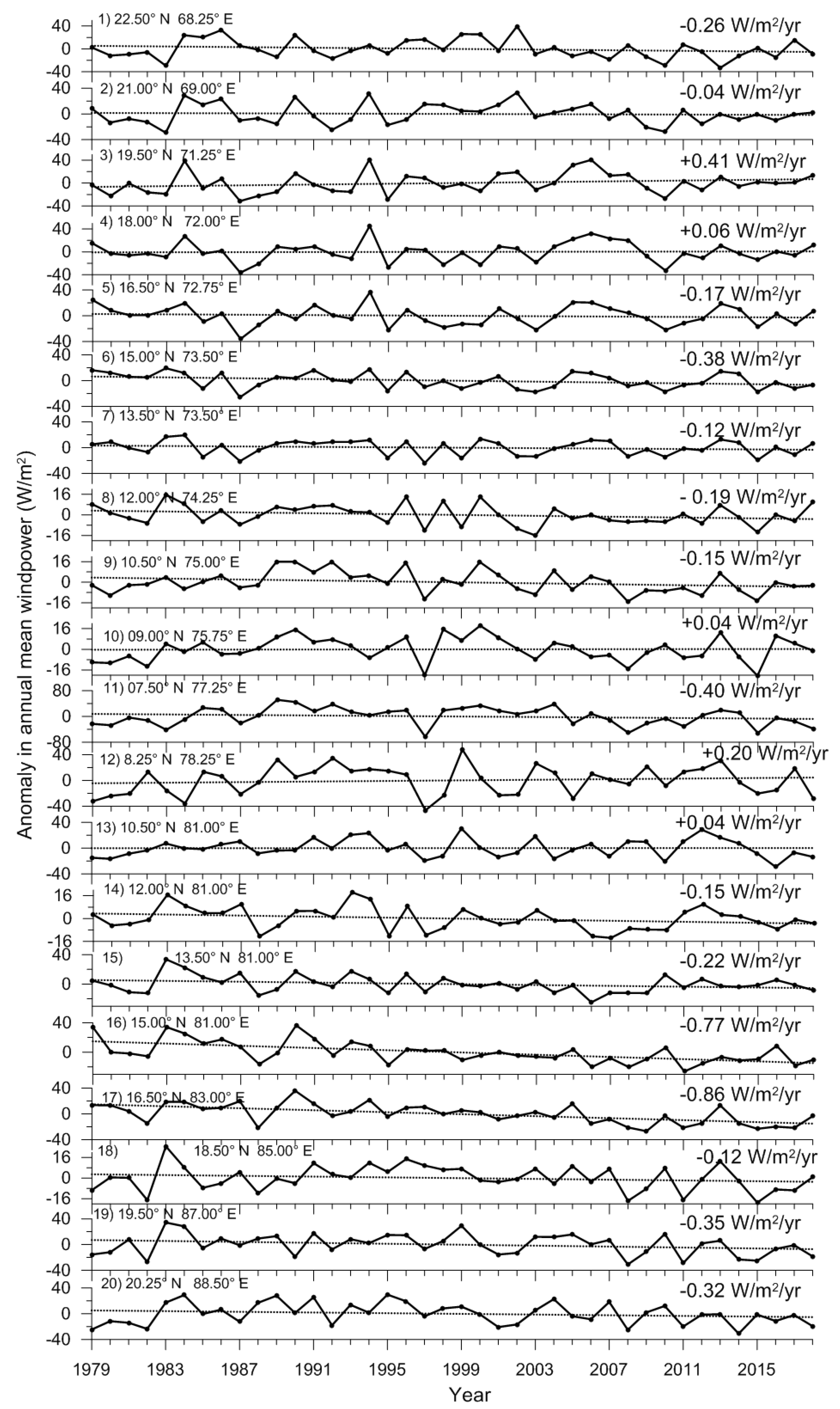
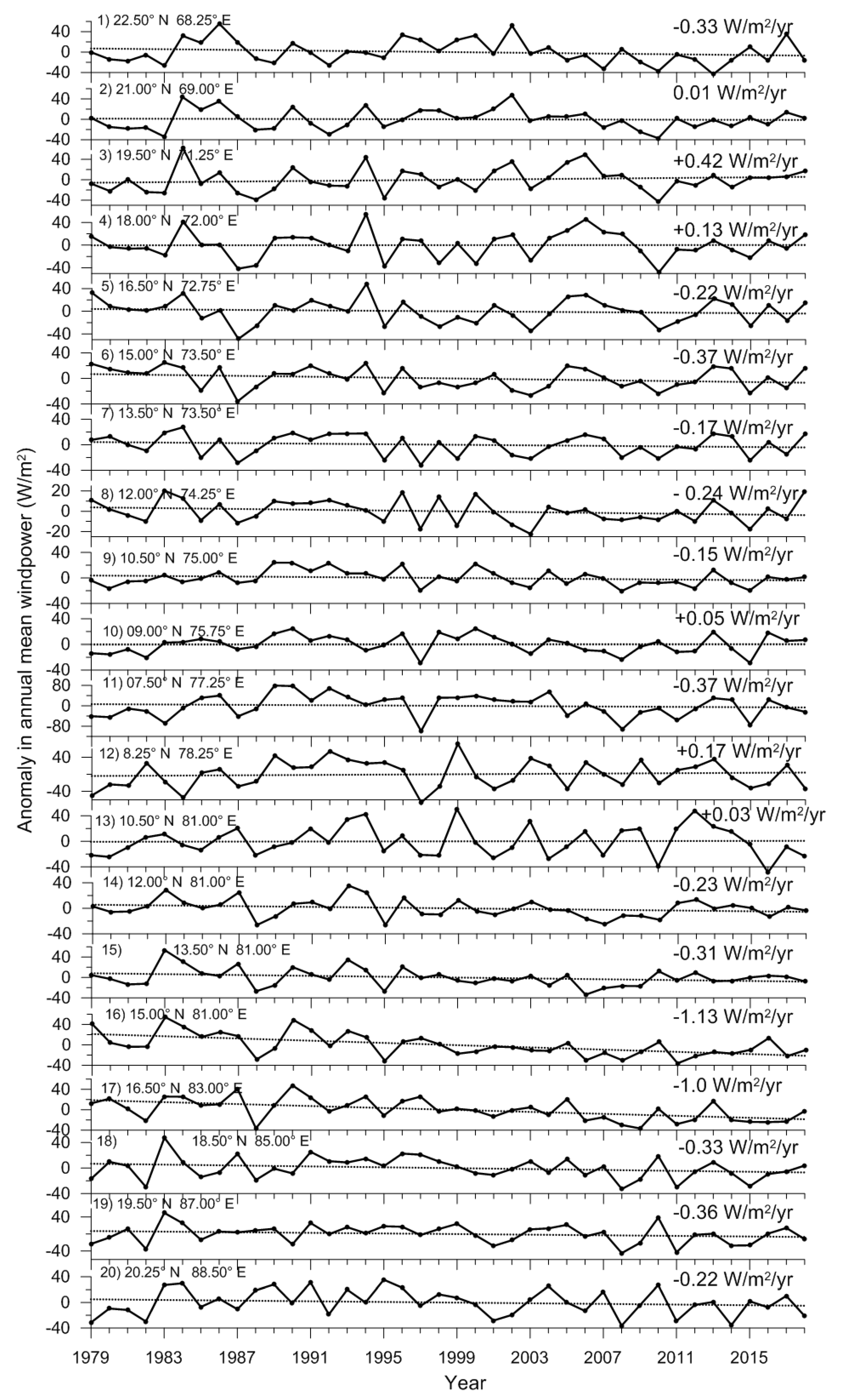
3.6. Long-Tterm Changes in Wind Power

Annual mean wind power anomalies computed for twenty locations at 10 m and 110.8 m above mean sea level over a 40 year period are shown in Figure 10 and Figure 11. Considerable inter-annual variations (up to 35%) were observed in the wind power rates along all the 20 locations for both heights and these variations were observed to be increasing with increased heights. At 10 m height, wind power anomalies vary from −62 to 51 W/m², whereas at 110.8 m, wind power anomalies vary from −98 to 79 W/m².

Trend analysis along these two levels suggests a negative trend in wind power rates for fifteen locations, whereas for five locations, trends are positive (Figure 10 and Figure 11). At 10 m, the trend varies from −0.86 to 0.4 W/m²/yr with its maximum negative trend along location 17 (−0.86 W/m²/yr), followed by location 16 (−0.77 W/m²/yr), and maximum positive trend along location 3 (0.41 W/m²/yr), followed by location 12 (0.20 W/m²/yr). At 110.8 m, trend varies from −1.13 to 0.17 W/m²/yr with its maximum negative trend along location 16 (−1.13 W/m²/yr), followed by location 17 (−1.06 W/m²/yr), and maximum positive trend along the location 12 (0.17 W/m²/yr), followed by location 4 (0.13 W/m²/yr). The highest positive trend in the annual mean 95 percentile and 99 percentile wind power is observed at location 3 at 10 m and 110.8 m of height (

Table 6. Linear trend in annual mean, 95 percentile and 99 percentile wind power at 10 and 110.8 m.

Location	Trend at 10 m (W/m2)			Trend at 110.8 m (W/m2)
	Mean	95 Percentile	99 Percentile	Mean	95 Percentile	99 Percentile
1	−0.26	−0.16	−1.48	−0.33	−0.03	−0.78
2	−0.04	0.03	−2.05	0.01	−0.39	−1.31
3	0.41	1.81	2.42	0.42	1.83	3.05
4	0.06	0.27	1.25	0.13	0.11	0.42
5	−0.17	−0.39	−0.66	−0.22	−0.49	−0.99
6	−0.38	−0.61	−0.69	−0.37	−0.79	−0.89
7	−0.12	−0.51	−1.88	−0.17	−0.63	−2.42
8	−0.19	−0.02	−0.58	−0.24	0.15	−0.48
9	−0.15	−0.11	0.83	−0.15	−0.05	1.50
10	0.04	0.01	0.29	0.05	−0.14	0.46
11	−0.40	−1.82	−2.15	−0.37	−2.04	−1.15
12	0.20	−0.29	−0.27	0.17	−0.78	0.01
13	0.04	−0.04	0.90	0.03	0.11	1.83
14	−0.15	−0.33	−0.16	−0.23	−0.43	−0.25
15	−0.22	−0.23	0.65	−0.31	−0.26	0.79
16	−0.77	−1.65	−2.83	−1.13	−2.36	−3.55
17	−0.86	−1.94	−2.42	−1.00	−2.78	−3.10
18	−0.12	−0.35	1.43	−0.33	−1.07	2.17
19	−0.35	−0.77	1.08	−0.36	−0.71	0.94
20	−0.32	0.15	−0.65	−0.22	0.28	−1.87

).

Wind power is the cube of wind speed, and a small change in wind speed can have significant changes in wind power. Declining trends in surface wind speeds along the eastern AS, central BoB and south–west BoB were previously reported by Anoop et al. [29], Shanas and Kumar [30] and George and Kumar [31]. Kumar and Anoop [32] reported weak declining trends in surface wind speeds along most of the locations in the shelf seas around India. A statistical significance test using the Mann Kendall test suggested that only four locations (locations 3, 6, 16, and 17) at 10 m and 110.8 m display a significant trend at a 90% confidence level. In contrast, other locations are significant at lower confidence levels (<80%).

Torralba et al. [33] suggest that the main drivers in the wind speed trends are the changes in large scale circulations. In Figure 10 and Figure 11 it is clearly evident that interannual variability appears to have some connections with ENSO, one of the prominent interannual modes of climate variability. For example, very strong El Niño years (1982–1983, 1997–1998, and 2015–2016) and strong/moderate El Niño years (1988–1989, 1999–2000, 2008–2009, and 2011–2012) over the past 40 years are associated with lower wind power rates for all the levels for most of the locations. Also, strong La Niña years (1988–1989, 1998–2000, 2007–2008, and 2010–2011) and moderate La Niña years (1995–1996 and 2011–2012) are associated with higher wind power rates for all the levels. The Indian Ocean is directly impacted by ENSO through Walker circulation [34], and their regional influence resulting in the reduction of wind speeds [35]. Using the annual averaged Oceanic Niño Index (ONI), correlation coefficients (R) with wind power rates at both heights for all of the 20 locations were estimated, and are shown in Figure 12. R value varies from −0.49 to 0.15 and −0.35 to 0.37 for 10 m and, 110.8 m, respectively. Maximum positive correlations are observed at 110.8 m (R = 0.37), with a confidence level of 95%, and the maximum negative correlation is observed at 10 m (R = −0.49, 95% confidence level). In the AS (locations 1–10), R values show a similar pattern, with comparatively larger values in 10 m than 110.8 m. However, in the BoB, correlations are negative at 10 m, particularly in locations 14–20, while at 110.8 m a positive correlation is observed. Hence, the inter-annual changes in wind power density were due to El Niño–Southern Oscillation events apart from that associated with variations in Indian summer monsoon.

4. Conclusions

Wind power in the Indian shelf seas shows distinct regional and seasonal differences. The monthly maximum wind power is in July in all locations along the eastern Arabian Sea compared to other months, since the intertropical convergence zone is located above the Indian landmass in this period. Wind power is at the maximum during the south-west monsoon and at minimum in the pre-monsoon period. Regions of higher wind power are found in locations 11 and 12. In contrast, the wind power in locations 7, 8, and 9 is poor above 250 W/m². Over the last 40 years, areas with high occurrence of wind power more than 50 W/m² were found in locations 11 to 13. Areas with a high occurrence of wind power over 200 W/m² are found at location 12. Since this location is situated between the Indian landmass and Sri Lankan landmass, the high wind power in this location is due to the wind channeled by land topography. The consistency of wind power in location 11 is better overall than that in other areas. The occurrence of exploitable wind speed is high (~80%) in southern locations throughout the year, and hence these locations are favourable for wind energy resource extraction. The total storage of wind energy in most of the shelf seas is above 0.7 × 10³ kWh/m², and location 12 has the highest (~ 3 × 10³ kWh/m²). The study shows that the inter-annual variation in wind power is up to 35% and the highest variation occurs at location 3. The trends of annual mean wind power along the Indian shelf seas over the last 40 years show a decreasing trend at many locations at heights of both 10 m and 110.8 m. The study also reveals that the long-term variation in wind power in the Indian Shelf seas is driven by ENSO, where the El Niño (La Niña) events are generally associated with lower (higher) wind power densities for both of the heights. This study provides informations on the wind power resources across the entire Indian shelf seas and its variations over the last 40 years, and will provide input for the planning of wind energy farms. The results presented in this study form the primary input for planning wind farms in the Indian shelf seas. Recently Amrutha and Kumar [36] reported the wave energy resources in the same locations in the Indian shelf seas, and the data presented in this article could be used for planning hybrid energy converters in the shelf seas of India.

References

1. Neill, S.P.; Hashemi, M.Z. Fundamentals of Ocean Renewable Energy; Academic Press: London, UK, 2018; p. 336. ISBN 9780128104484. [Google Scholar]
2. Kåberger, T. Progress of renewable electricity replacing fossil fuels. Glob. Energy Interconnect. 2018, 1, 48–52. [Google Scholar] [CrossRef]
3. GWEC. Annual Market Update; Global Wind Report; The Global Wind Energy Council (GWEC): Brussels, Belgium, 2018. [Google Scholar]
4. GWEC. Global Wind Statistics 2016. 2017. Available online: www.gwec.net (accessed on 23 August 2019).
5. Blaabjerg, F.; Ma, K. Wind Energy Systems. Proc. IEEE 2017, 105, 2116–2131. [Google Scholar] [CrossRef] [Green Version]
6. Sheridan, B.; Baker, S.D.; Pearre, N.S.; Firestone, J.; Kempton, W. Calculating the offshore wind power resource: Robust assessment methods applied to the U.S. Atlantic Coast. Renew. Energy 2012, 43, 224–233. [Google Scholar] [CrossRef]
7. Hasager, C.B.; Mouche, A.; Badger, M.; Bingöl, F.; Karagali, I.; Driesenaar, T.; Stoffelen, A.; Peña, A.; Longépé, N. Offshore wind climatology based on synergetic use of Envisat ASAR, ASCAT and QuikSCAT. Remote Sens. Environ. 2015, 156, 247–263. [Google Scholar] [CrossRef]
8. Chang, R.; Zhu, R.; Badger, M.; Hasager, C.B.; Xing, X.; Jiang, Y. Offshore Wind Resources Assessment from Multiple Satellite Data and WRF Modeling over South China Sea. Remote Sens. 2015, 7, 467–487. [Google Scholar] [CrossRef] [Green Version]
9. Guo, Q.; Xu, X.; Zhang, K.; Li, Z.; Huang, W.; Mansaray, L.R.; Liu, W.; Wang, X.; Gao, J.; Huang, J. Assessing Global Ocean Wind Energy Resources Using Multiple Satellite Data. Remote Sens. 2018, 10, 100. [Google Scholar] [CrossRef] [Green Version]
10. Zheng, C.; Xiao, Z.; Yuehua, P.; Li, C.; Du, Z. Rezoning global offshore wind energy resources. Renew. Energy 2018, 129, 1–11. [Google Scholar] [CrossRef]
11. Murthy, K.S.R.; Rahi, O.P. A comprehensive review of wind resource assessment. Renew. Sustain. Energy Rev. 2016, 72, 1320–1342. [Google Scholar] [CrossRef]
12. Tank, V.; Bhutka, J.; Harinarayana, T. Wind Energy Generation and Assessment of Resources in India. J. Power Energy Eng. 2006, 4, 25–38. [Google Scholar] [CrossRef] [Green Version]
13. Zheng, C.; Pan, J.; Li, J. Assessing the China Sea wind energy and wave energy resources from 1988 to 2009. Ocean Eng. 2013, 65, 39–48. [Google Scholar] [CrossRef]
14. Olauson, J. ERA5: The new champion of wind power modelling? Renew. Energy 2018, 126, 322–331. [Google Scholar] [CrossRef] [Green Version]
15. Hersbach, H.; Dee, D. ERA5 reanalysis is in production. ECMWF Newsl. 2016, 147, 7. [Google Scholar]
16. Bosch, J.; Staffell, I.; Hawkes, A.D. Temporally explicit and spatially resolved global offshore wind energy potentials. Energy 2018, 163, 766–781. [Google Scholar] [CrossRef]
17. Arent, D.; Sullivan, P.; Heimiller, D.; Lopez, A.; Eurek, E.; Badger, J.; Jørgensen, H.; Kelly, M. Improved Offshore Wind Resource Assessment in Global Climate Stabilization Scenarios. Technical Report: NREL/National Renewable Energy Laboratory (NREL), TP-6A20–55049; 2012; pp. 1–24. Available online: http://www.nrel.gov/docs/fy13osti/55049.pdf (accessed on 23 August 2019).
18. Wind Europe. Offshore Wind in Europe. Key Trends and Statistics 2018; Technical Report; Wind Europe: Brussels, Belgium, 2018; Available online: https://windeurope.org (accessed on 3 December 2019).
19. GWEC. Global Wind 2018 Report; Technical Report; Global Wind Energy Council: Brussels, Belgium, 2018; Available online: http://www.gwec.net (accessed on 3 December 2019).
20. Sanjeev, G.; Paresh, C.D. Offshore wind power resource assessment using Oceansat-2 scatterometer data at a regional scale. Appl. Energy 2016, 176, 157–170. [Google Scholar] [CrossRef]
21. Calif, R.; Schmitt, F. Modeling of atmospheric wind speed sequence using a lognormal continuous stochastic equation. J. Wind Eng. Ind. Aerodyn. 2012, 109, 1–8. [Google Scholar] [CrossRef]
22. Ramon, J.; Lledo, L.; Torralba, V.; Soret, A.; Doblas-Reyes, F.J. What global reanalysis best represents near-surface winds? Q. J. R. Meteorol. Soc. 2019, 145, 3236–3251. [Google Scholar] [CrossRef] [Green Version]
23. Findlater, J. A major low-level air current near the Indian Ocean during the northern summer. Quart. J. R. Meteorol. Soc. 1969, 95, 362–380. [Google Scholar] [CrossRef]
24. Sirisha, P.; Remya, P.G.; Modi, A.; Tripathy, R.R.; Balakrishnan Nair, T.M.; Rao, B.V. Evaluation of the impact of high-resolution winds on the coastal waves. J. Earth Syst. Sci. 2019, 128, 226. [Google Scholar] [CrossRef] [Green Version]
25. Chowdhury, S.; Zhang, J.; Messac, A.; Castillo, L. Unrestricted wind farm layout optimization (UWFLO): Investigating key factors influencing the maximum power generation. Renew. Energy 2012, 38, 16–30. [Google Scholar] [CrossRef]
26. Aboobacker, V.M.; Shanas, P.R. The climatology of shamals in the Arabian Sea–Part 1: Surface winds. Int. J. Climatol. 2018, 38, 4405–4416. [Google Scholar] [CrossRef]
27. Anoop, T.R.; Shanas, P.R.; Aboobacker, V.M.; Sanil Kumar, V.; Nair, L.S.; Prasad, R.; Reji, S. On the generation and propagation of Makran swells in the Arabian Sea. Int. J. Climatol. 2020, 40, 585–593. [Google Scholar] [CrossRef]
28. Naseef, T.M.; Kumar, V.S. Climatology and trends of the Indian Ocean surface waves based on 39-year long ERA5 reanalysis data. Int. J. Climatol. 2020, 40, 979–1006. [Google Scholar] [CrossRef]
29. Anoop, T.R.; Kumar, V.S.; Shanas, P.R.; Johnson, G. Surface wave climatology and its variability in the north Indian Ocean Based on ERA-interim reanalysis. J. Atmos. Ocean. Technol. 2015, 32, 1372–1385. [Google Scholar] [CrossRef] [Green Version]
30. Shanas, P.R.; Kumar, V.S. Trends in surface wind speed and significant wave height as revealed by ERA-Interim wind wave hindcast in the Central Bay of Bengal. Int. J. Climatol. 2015, 35, 2654–2663. [Google Scholar] [CrossRef]
31. George, V.; Kumar, V.S. Wind-wave measurements and modelling in the shallow semi-enclosed Palk Bay. Ocean Eng. 2019, 189, 106401. [Google Scholar] [CrossRef]
32. Kumar, V.S.; Anoop, T.R. Spatial and temporal variations of wave height in shelf seas around India. Nat. Hazards 2015, 78, 1693–1706. [Google Scholar] [CrossRef]
33. Torralba, V.; Doblas-Reyes, F.J.; Gonzalez-Reviriego, N. Uncertainty in recent near-surface wind speed trends: A global reanalysis intercomparison. Environ. Res. Lett. 2017, 12, 114019. [Google Scholar] [CrossRef]
34. Klein, S.A.; Soden, B.J.; Lau, N.C. Remote sea surface temperature variations during ENSO: Evidence for a tropical atmospheric bridge. J. Clim. 1999, 12, 917–932. [Google Scholar] [CrossRef] [Green Version]
35. Wyrtki, K. An Estimate of Equatorial Upwelling in the Pacific. J. Phys. Oceanogr. 1981, 11, 1205–1214. [Google Scholar] [CrossRef] [Green Version]
36. Amrutha, M.M.; Kumar, V.S. Changes in Wave Energy in the Shelf Seas of India during the Last 40 Years Based on ERA5 Reanalysis Data. Energies 2020, 13, 115. [Google Scholar] [CrossRef] [Green Version]
Figure 1. Locations considered in the study. The shade is the bathymetry of the ocean in metres.
Energies 13 02295 g001
Figure 2. Monthly mean wind speed at 110.8 m height from the fifth generation European Centre for Medium-Range Weather Forecasts (ECMWF) atmospheric reanalyses of the global climate (ERA5) data, and that estimated following power law (Equation (1)) at different locations.
Energies 13 02295 g002
Figure 3. Spatial distribution of seasonally averaged wind power density at 10 m above mean sea level during pre-monsoon, SW monsoon, post-monsoon and annual.
Energies 13 02295 g003
Figure 4. Monthly mean wind power density at different locations along eastern Arabian Sea and western Bay of Bengal.
Energies 13 02295 g004
Figure 5. Maximum, minimum, and annual mean wind power density at 110.8 m above the surface in different years at locations 1 to 20.
Energies 13 02295 g005
Figure 6. Percentage occurrence of wind power along eastern Arabian Sea and western Bay of Bengal during south-west monsoon period.
Energies 13 02295 g006
Figure 7. Seasonal and annual mean wind power density along western Bay of Bengal and Arabian Sea at (a) 10 m and (b) 110.8 m height.
Energies 13 02295 g007
Figure 8. Time series plot of wind speed and direction in year 2018 at locations 8, 11, and 12.
Energies 13 02295 g008
Figure 9. Rose diagram showing the directional distribution of wind power at a height of 10 m in the different locations studied.
Energies 13 02295 g009
Figure 10. Anomaly in annual mean wind power at 10 m height. The trend during the 40 years is also indicated in the figure.
Energies 13 02295 g010
Figure 11. Anomaly in annual mean wind power at 110.8 m height. The trend during the 40 years is also indicated in the figure.
Energies 13 02295 g011
Figure 12. Correlation coefficients between annual averaged Oceanic Niño Index (ONI) and wind power at 10 m and 110.8 m for all of the 20 locations.
Energies 13 02295 g012