Abstract
A q-rung orthopair fuzzy set (q-ROFS), an extension of the Pythagorean fuzzy set (PFS) and intuitionistic fuzzy set (IFS), is very helpful in representing vague information that occurs in real-world circumstances. The intention of this article is to introduce several aggregation operators in the framework of q-rung orthopair fuzzy numbers (q-ROFNs). The key feature of q-ROFNs is to deal with the situation when the sum of the qth powers of membership and non-membership grades of each alternative in the universe is less than one. The Einstein operators with their operational laws have excellent flexibility. Due to the flexible nature of these Einstein operational laws, we introduce the q-rung orthopair fuzzy Einstein weighted averaging (q-ROFEWA) operator, q-rung orthopair fuzzy Einstein ordered weighted averaging (q-ROFEOWA) operator, q-rung orthopair fuzzy Einstein weighted geometric (q-ROFEWG) operator, and q-rung orthopair fuzzy Einstein ordered weighted geometric (q-ROFEOWG) operator. We discuss certain properties of these operators, inclusive of their ability that the aggregated value of a set of q-ROFNs is a unique q-ROFN. By utilizing the proposed Einstein operators, this article describes a robust multi-criteria decision making (MCDM) technique for solving real-world problems. Finally, a numerical example related to integrated energy modeling and sustainable energy planning is presented to justify the validity and feasibility of the proposed technique.
1. Introduction
Currently, creating a sustainable energy policy for countries poses a considerable challenge. It raises several issues such as energy policy definition and planning [1], the choice of energy sources [2], and the assessment of energy supply technologies [3]. Due to the critical, complex, subjective, and poorly structured nature of the issues themselves, many of the scientists’ contributions are directed to the area of building objective models of decision support. The reason for this phenomenon should be sought in the fact that modeling this class of problems requires correct mapping not only of the assessed alternatives/variants or scenarios. In such a case, experts must also consider the consequences of analyzing the decision problem from different perspectives and points of view taking into account several conflicting criteria [4]. For example, a sustainable energy planning process requires taking into account several environmental, social, and economic groups of factors in the decision making process [5]. Often, the shape of the final ranking is additionally influenced by the presence of interest groups [6], and this factor also requires objectification and correct mapping in the developed model [7]. The availability of measurement data of the model and their imprecision [8] (together with the preference of the decision makers uncertainty [9]) are not without significance. At the same time, it is a widely raised and still valid research challenge [10].
From the methodological point of view, current literature studies confirm that an extension of the decision support process beyond the classic optimization model of a single objective function is commonly accepted, described on a set of acceptable solutions [4]. This extension makes it possible to undertake multi-criteria problems, focusing on obtaining a solution that satisfies many, often conflicting goals. The existence of many criteria, conflicts between criteria, and the complex, subjective, and poorly structured nature of the decision problem constitute the paradigm of multi-criteria decision support [11]. It is on these foundations that many multi-criteria decision making (MCDM) [12] methods have been developed. The actual state-of-the-art in this area clearly confirms that MCDM methods handle the problem mentioned above practically and effectively. The analysis of the literature indicates the prevalence of the use of MCDM methods in energy decision making issues. MCDM methods are used as practical and useful tools to solve problems related to decision making on energy policy making [13] or RES technology selection and assessment [14]. This fact can be easily confirmed by review and meta-analysis papers like Løken [15], Martín-Gamboa et al. [16], Wang et al. [5], and Arce et al. [17]. These papers show the multitude of both practical problems in the field of energy policy and MCDM techniques used as a formal background for the models developed.
The literature studies also confirm the widespread use of fuzzy developments (based on the theory of fuzzy sets) of MCDM methods in energy issues [1,18]. The essence of this approach is based on the fact that fuzzy number theory models express the uncertainty in individual opinions to obtain more sensitive, concrete, and realistic modeling results [19]. This topic is widely discussed in the literature [20]. Many new extensions of MCDM methods are being developed with the use of successive tools of different generalizations of fuzzy sets that are being designed to handle the uncertain decision making environment [21]. It is worth noting that despite a large number of methodological and practical works in this area, the authors’ conclusions indicate the need to improve the workshop of existing models supporting this decision making process [18]. The reasons for this, apart from the obvious contradiction of the goals here, are a complex and multi-level set of criteria or natural uncertainty of measurement data and decision makers preferences, which address the numerous difficulties in accurately reflecting the MCDM model [19]. In response to the aforementioned shortcomings in the current paper, we developed a new robust MCDM technique based on Einstein operators with q-rung orthopair fuzzy numbers. We propose the score function, accuracy function, and certainty function for ranking q-rung orthopair fuzzy numbers (q-ROFNs). We present the mathematical procedure of our approach to solving sustainable energy planning problems in Pakistan.
The rest of this paper is organized as follows. Section 2 contains a literature review of the MCDM method’s usage in RES domain decision problems by using uncertain and imperfect information. In Section 3, we discuss the concept of q-rung orthopair fuzzy sets (q-ROFSs). We define some operational laws, basic aggregation operators, the score function, and the accuracy function for q-rung orthopair fuzzy numbers (q-ROFNs). In Section 4, we discuss the concept of the t-norm and t-conorm and Einstein operational laws for q-ROFSs. In Section 5, we introduce some new q-rung orthopair fuzzy Einstein aggregation operators. In Section 6, we develop q-ROFNs based multi-criteria decision making method and discuss integrated energy modeling and sustainable energy policy. In Section 7, we give the conclusion of the research work.
2. Literature Review
2.1. MCDM Background in the Sustainability Domain
The analysis of the genesis and primal areas of usage of multi-criteria decision support methods emphasizes their dynamic development, which began in the 1970s. In the 1980s, they were already amongst the primary management support tools. To confirm this fact, the work presented by Teckle [22] included the current state of the research, along with an extended analysis of the applications of MCDM methods in various management problems. Examples of areas of effective use of MCDM encompassed management of water resources [23,24], including waste (sewage) [25], management of forest resources [26] (more broadly environmental [27,28]), many decision problems in transport [29] and logistics [30], as well as model issues for the MCDM problems of land parcels [31] or human resource planning [32]. It is possible to point out many applications of multi-criteria decision support methods in the area of strategic problems, such as the evaluation of projects [33], plans and strategies [34], or the choice of a specific policy direction [35], selection and evaluation of public facilities (e.g., schools [36], hospitals [37]), regional development planning [38], capital investments [39] and budgeting [40], planning and implementation of the production process [41], economic policy [42], evaluation of information systems [43], or dedicated military objectives [44]. At the moment, the area of usage of MCDM methods has become extremely broad, and apart from the model above-mentioned classes of management problems, it covers the remaining spheres of economic practice, science, as well as everyday human decision problems.
In the last decade, the concept of sustainability has been one of the most important research topics. Generally, the term sustainability refers to social, economic, and environmental [45] aspects to ensure prosperity, environmental protection, and social unity [46]. According to the scientific literature, the sustainability concept has a multi-disciplinary form and a multi-faceted nature [47]. In recent years, the topics related to sustainability, sustainability development, and sustainability management have become the main factors determining the majority of business and organizational activities. To confirm this, many global, international, national, and regional strategies are based on sustainability aspects [48]. Sustainable decision making combines management theories and the principles of sustainability, considering environmental, social, and economic factors in the decision making process [5]. Therefore, making decisions in the area of sustainable development requires the reconciliation of contradictory goals. Frequently, decisions have a multi-level and multi-faceted nature, requiring the participation and involvement of many shareholders. Thus, the need for including conflicting goals, conflicting criteria, as well as many stakeholders in one decision making process causes the modeling of sustainability problems to be often carried out using MCDM methods. This fact is confirmed by many literature studies presenting various decision problems related to sustainability, yet successfully modeled using MCDM methods. For example, the problems include assessment of sustainability processes in a selected area [49], resource planning, corporate policy and strategy [50], public policy modeling [51], spatial planning, economic [52], or government policy planning [53], measuring of the sustainable information society [54], or modeling of sustainable population growth and urbanization problems [55,56].
Moreover, MCDM methods have also been applied in sustainable modeling of the consumer market [57], optimization of the sustainable portfolio [58], modeling of the sustainable use of resources [59], maximizing user conversion [60], or modeling of industrial development and the energy crisis [61]. Besides, in the area of sustainable company management, the applicability of the MCDM methods was confirmed in such management problems as: finance, information technology, logistics (including sustainable supply chain management [62] and the choice of a sustainable supplier) [4]. The ability to aggregate data and generate synthetic assessments of individual decision making variants allows MCDM methods to create sustainable development indicators for the energy industry [63], water areas [64], rural areas [52], the development of countries [65], agricultural development [66], or urban areas [55].
2.2. MCDM Methods in Energy Policy Modeling
In recent years, a growing interest in renewable energy sources (RES) has been observed. Determinants of such a situation can be found in, among others, the development of technologies and the search for the independence of national economies of many countries from conventional energy sources [67]. Furthermore, the progressive decline in the resources of natural energy forces changes in macro and micro energy strategies, while increasing their prices on the global market. It is worth mentioning that renewable energy sources can be used almost anywhere in the world. However, the main problem corresponds to the justification of the economic, technological, environmental, and social correctness of the location and construction of infrastructure using this type of resource. For instance, an improperly located farm can be a source of negative environmental and social impacts.
The inclusion of the aforementioned environmental imperatives in energy policy planning, as well as the addition of pro-social factors have resulted in the need to reconcile conflicting objectives and different stakeholders in the process of the planning and evaluation of energy policy in regions or countries. Some of the essential tools for model structuring and problem-solving are the MCDM methods [68]. Numerous literature review studies confirmed this fact [15,16,17,69]. What is important is that the American and European schools’ approaches to the multi-criteria decision support have become very popular in this area [70]. The popularity of “American school” methods, based on value/utility theory (usually single synthesizing criterion), has been confirmed, for example in [14,71]. Among them, the analytic hierarchy process (AHP) method is widely used. It is characterized by a relatively simple computational algorithm and, at the same time, the possibility of reflecting well the complex, hierarchical structure of this class of decision making problems. Numerous works in the field of energy policy using the AHP method can be pointed out, and examples of them concern in particular the selection of renewable energy sources for sustainable development [72], strategic renewable energy resources’ selection [73], energy source policy assessment [74], or sustainable energy planning [75]. The same group of methods (schools) includes TOPSIS and VIKOR. They are based on similar principles, and their application additionally allows for the construction of so-called “reference points” (ideal and anti-ideal solution). These methods have also proven effective in the assessment of economic and environmental energy performance [76], optimization of power generation systems [77], sustainable energy-storing optimization [78], or selecting sustainable energy conversion technologies [79]. It is worth noting that the methods of the “American school” are not entirely appropriate in modeling sustainable energy issues [80]. This is directly related to the fact that these methods are characterized by an undesirable effect of linear compensation (substitution) of criteria, which in practice significantly hinders and often makes it impossible to meet the paradigm of so-called “strong sustainability” [81]. The methods of the so-called “European school” are characterized by lower levels of criteria compensation (partial compensation/non-compensation), and thus stronger fulfillment of the strong sustainability paradigm. The most popular outranking methods include ELECTRE and PROMETHEE [82]. The techniques from the ELECTRE family show effectiveness in modeling problems, in which there is an under-specification of preferential information [83], and modeling this under-specification is done using pseudo-criteria (criteria with thresholds) and outranking relations [83], which constitute the foundation for building the final outranking graph. The methods of the PROMETHEE family are characterized by the same formal assumptions (outranking relation). However, the final ranking is in the form of alternative quantitative assessments [84]. Examples of the effective use of these methods in energy policy include the evaluation of power plants [85], the evaluation of sustainable energy sources [86], rank policies [87], or investment risk evaluation for new energy resources [88]. Regardless of the methods indicated, the need to objectify the models leads researchers towards building hybrid approaches. This means that several MCDM methods are used in one model or several models are constructed for benchmarking purposes. Such procedures in the area of energy policy can be found, for example, in the works [79,89,90,91].
A detailed analysis of the works indicates that apart from the proper selection of the appropriate MCDM method, the current challenge in this class of problems remains the accurate modeling of the data, the preferences of the interveners in the model, and more importantly, their imprecision [83]. It constitutes the correctness of the entire decision making process and the quality of the final recommendation [11].
2.3. MCDM Based Uncertain Data Modeling
For many years, the issue of vague and imperfect information has been at the forefront. Information aggregation is the key factor for decision management in the areas of business, management, engineering, psychology, social sciences, medical sciences, and artificial intelligence. Traditionally, the knowledge about an alternative has been believed to be considered as simple numbers. Nevertheless, knowledge cannot be accessed in a simple form at any time in the modern world. It is very important to address data inconsistencies in order to deal with these conditions. Zadeh [92] initiated the concept of the fuzzy set by means of the membership function. A fuzzy set is a significant mathematical model to define and assemble the objects whose boundaries are elusive by utilizing membership grades. Atanassov [93] introduced the intuitionistic fuzzy set (IFS) as an extension of the fuzzy set. Yager [94,95,96] introduced the Pythagorean fuzzy set (PFS) as an extension of Atanassov’s intuitionistic fuzzy set. Bashir et al. [97] discussed the convergences for intuitionistic fuzzy set theory as important fundaments to extend MCDM methods. A Pythagorean fuzzy number (PFN) is superior to an intuitionistic fuzzy number (IFN). Yager further introduced the idea of the q-rung orthopair fuzzy set (q-ROFS) as the extension of the Pythagorean fuzzy set (PFS) [98]. A q-rung orthopair fuzzy number (q-ROFN) is superior to both IFN and PFN because IFN and PFN both may be regarded as q-ROFN, but not conversely (see [96,98]). Yager [99] introduced the concept of ordered weighted averaging aggregation operators for MCDM. Akram et al. [100,101,102,103] proved the usefulness of m-polar fuzzy soft rough sets, neutrosophic incidence graphs, and m-polar fuzzy ELECTRE-Iin decision making problems. Ali et al. [104] presented new abilities of soft sets and rough sets with fuzzy soft sets. Garg and Arora [105,106,107,108] established certain concepts of IFsoft power and dual hesitant fuzzy soft aggregation operators. Hashmi et al. [109] introduced the notion of the m-polar neutrosophic set and m-polar neutrosophic topology and their applications to MCDM in medical diagnosis and clustering analysis. Hashmi and Riaz [110] introduced a new way to handle the censuses process by using the Pythagorean m-polar fuzzy Dombi aggregation operators. In Kumar and Garg [111], a new extension of the well-known TOPSIS method based on pair set analysis with the use of interval-valued intuitionistic fuzzy set theory was presented. Karaaslan [112] introduced neutrosophic soft sets with applications in decision making. Naeem et al. [113] introduced Pythagorean fuzzy soft MCGDM methods based on TOPSIS, VIKOR, and aggregation operators. The hybrid concept based on Pythagorean m-polar fuzzy sets and the TOPSIS method was presented in Naeem et al. [114]. Peng and Yang [115] discussed some new results of PFS and defined the Pythagorean fuzzy number (PFN). Fuzzy information measures and their applications were introduced in Peng et al. [116]. Peng and Selvachandran [117] developed state-of-the-art and future directions for PFS. The new concept of the Pythagorean fuzzy soft set (covering practical areas) was presented by [118]. Pend and Dau [119] investigated the use of single-valued neutrosophic MCDMto extend the MABACand TOPSIS methods. In their work, they used a new similarity coefficient using the score function. Riaz et al. [120,121,122] introduced the N-soft topology and soft rough topology with applications to group decision making. Riaz and Hashmi [123] presented the concept of the cubic m-polar fuzzy set application in multi-attribute group decision making (MAGDM) with application to the agribusiness domain.
MCDM problem solving based on the notion of linear Diophantine fuzzy set (LDFS) was presented in [124]. LDFS is superior ti IFS, PFS, and q-ROFS. Riaz and Hashmi [125] introduced novel concepts of MCDM based on soft rough Pythagorean m-polar fuzzy sets and Pythagorean m-polar fuzzy soft rough sets. New approaches based on the idea of bipolar fuzzy soft topology, cubic bipolar fuzzy sets, and cubic bipolar fuzzy ordered weighted geometric aggregation were also presented in [126,127,128]. Studies confirmed a broad spectrum of practical usage of the given extensions.
They presented various illustrations and decision making applications of these concepts by using different algorithms. In [129], the useful concept of bipolar fuzzy soft mappings was presented. The same idea was successfully applied in the new TOPSIS method extension and its applications to MCGDM [130].
Xu proposed the IF aggregation operators concept in [131]. In the book [132], Xu and Cai introduced the theory and applications of the intuitionistic aggregation of fuzzy information. Xu [133] investigated hesitant fuzzy sets theory and different ways of aggregation knowledge. The next stage of development was the research conducted by Ye [134], who showed an approach based on interval-valued hesitant fuzzy prioritized weighted aggregation (IVHFPWA) operators and their practical application to MCDM problems. The linguistic neutrosophic cubic numbers were first presented as an extended approach to solving MCDM problems in [135]. Two interesting approaches related to soft rough covering and rough soft hemirings were proposed by Zhan et al. [136,137]. Zhang et al. [138,139,140] proposed much work for using uncertain data to solve MCDM problems. As a result of their work, they presented fuzzy soft -covering based fuzzy rough sets, covering on generalized intuitionistic fuzzy rough sets, and fuzzy soft coverings based fuzzy rough sets. Ali [141] presented two new approaches of q-rung orthopair fuzzy sets based on L-fuzzy sets and the notion of orbits. Liu and Wang [142] presented some q-rung orthopair fuzzy aggregation operators and their application to MCDM. Liu et al. [143] developed a ranking range based approach to MCDM under incomplete knowledge, and it was verified in the venture investment evaluation.
3. Preliminaries
In this section, the conceptual ideas related to q-ROFS are given that are used in the rest of the paper.
Definition 1
([98]). A q-rung orthopair fuzzy set (q-ROFS) in a finite universe ℧ is an object of the form:
where and represent the degree of membership and the degree of non-membership of the element , respectively, to the set with the condition:
and the degree of indeterminacy is given as:
For each , a basic element of the form in a q-ROFS, denoted by , is called the q-rung orthopair fuzzy number (q-ROFN). It can be written as .
Operational Laws on q-Rung Orthopair Fuzzy Numbers
Definition 2
([142]). Let and be q-ROFNs. Then:
- (1)
- (2)
- (3)
- (4)
- (5)
- (6)
- (7)
Definition 3
([142]). Assume that is a family of q-ROFNs, and , if:
where Λ is the set of all q-ROFNs, is the weight vector of such that , and the sum of the components of must be equal to one. Then, the q-ROFWA is called the q-rung orthopair fuzzy weighted average operator.
Based on q-ROFNs operational rules, we can also consider q-ROFWA with Theorem 1.
Theorem 1.
Let be the family of q-ROFNs; we can find by:
Definition 4.
Assume that is the family of , and , if:
where is the set of all is the weight vector of such that , and the sum of the components of must be equal to one. Then, the is called the q-rung orthopair fuzzy weighted geometric operator. On the basis of the operational laws of q-ROFNs, we can also find by the theorem below.
Theorem 2.
Let be the family of q-ROFNs; we can find by:
Definition 5.
Suppose is a q-ROFN, then a score function of is defined as:
. The score of a q-ROFN defines its ranking, i.e., a high score defines a high preference of q-ROFN. However, the score function is not useful in many cases of q-ROFN. For example, let us consider and to be two q-ROFN. If we take the value of q to be two, then , i.e, the score functions of and are the same. Therefore, to compare the q-ROFNs, it is not necessary to rely on the score function.
We add a further method, the accuracy function, to solve this issue.
Definition 6.
Suppose is a q-ROFN, then an accuracy function of is defined as:
. The high value of accuracy degree defines the high preference of .
Again, consider and to be two q-ROFNs. Then, their accuracy functions are and ,so by the accuracy function, we have .
Definition 7.
Let and be any two q-ROFN and be the score functions of and , and be the accuracy functions of and , respectively, then:
- (1)
- If , then
- (2)
- If , then:
- if , then ,
- if , then .
4. Einstein Operational Laws of q-ROFNs
We will give an overview of the t-norm and t-conorm in this section and give examples relevant to these norms. Some of the properties of Einstein operations are given on q-ROFNs.
For the first time in the sense of probabilistic metric spaces, triangular norms have been adopted as we use them today. Throughout decision making, statistics, and theories on non-additive measures and cooperative games, they also play a significant role. Many parameterized t-norm families are renowned functional equation solutions. T-norms are used in fuzzy set theory at the intersection of two fuzzy sets. For modeling disjunction or union, t-conorms are used. These are a simple interpretation of the conjunction and disjunction in mathematical fuzzy logic semantics and are used in MCDM to combine criteria.
A triangular norm (t-norm) is a binary operation ✠ that satisfies the following conditions at the interval :
- (i)
- (ii)
- (iii)
- if and , then
- (iv)
- (neutral element one) and
Here, some famous examples of the t-norm are given:
- (minimum or Gdel t-norm)
- (product t-norm)
- (Lukasiewicz t-norm)
No t-norm can attain greater values than . The idempotents of a t-norm ✠ are those ℵ satisfying . The bounds zero and one are trivial idempotents. A t-norm is called Archimedean if each sequence , where and , converges to zero. A continuous t-norm is Archimedean iff it has no idempotents between zero and one. A continuous Archimedean t-norm is called strict if for all . Continuous Archimedean t-norms that are not strict are called nilpotent. The product t-norm is strict, and the Lukasiewicz t-norm is nilpotent.
A triangular conorm (t-conorm) is a binary operation that satisfies the following conditions at the interval :
- (i)
- (ii)
- (iii)
- if and , then
- (iv)
- (neutral element zero) and
Here, some famous examples of t-conorm are given:
- (maximum or Gdel t-conorm)
- (product t-conorm)
- (Lukasiewicz t-conorm)
No t-conorm can attain smaller values than . If ✠ is a t-norm, then is a t-conorm, and vice versa. Thus, we obtain a dual pair of a t-norm and a t-conorm. There are several types of groups of t-norms and t-conorms that can be chosen to construct the intersections and unions. Einstein sums and Einstein products are good alternatives for algebraic sums and algebraic products because they provide a very smooth approximation. Einstein sums and products are examples of t-norms and t-conorms and are defined as follows in the q-ROF setting.
Definition 8.
Let and be q-ROFNs and be any real number, then:
- (i)
- (ii)
- (iii)
- (iv)
- (v)
- (vi)
- (vii)
Theorem 3.
Let and be q-ROFNs and be any real number, then:
- (i)
- (ii)
- (iii)
- (iv)
- (v)
- (vi)
- (vii)
- (viii)
Proof.
See Appendix A.1. □
Theorem 4.
Let and be q-ROFNs, then:
- (i)
- (ii)
- (iii)
- (iv)
- (v)
- (vi)
Proof.
This is a trivial case. We omit it here. □
Theorem 5.
Let , and be q-ROFNs, then:
- (i)
- (ii)
- (iii)
- (iv)
- (v)
- (vi)
Proof.
This is a trivial case. We omit it here. □
5. q-Rung Orthopair Fuzzy Einstein Aggregation Operators
In this section, we introduce several new Einstein operators for q-ROFNs, namely the q-rung orthopair fuzzy Einstein weighted averaging (q-ROFEWA) operator, the q-rung orthopair fuzzy Einstein ordered weighted averaging (q-ROFEOWA) operator, the q-rung orthopair fuzzy Einstein weighted geometric (q-ROFEWG) operator, and the q-rung orthopair fuzzy Einstein ordered weighted geometric (q-ROFEOWG) operator.
5.1. q-Rung Orthopair Fuzzy Einstein Weighted Averaging Operator
Definition 9.
Let be the family of q-ROFNs and (q-ROFEWA) if,
where Λ is the set of all , is the weight vector of such that , and the sum of the components of must be equal to one. Then, the q-ROFEWA is called the q-rung orthopair fuzzy Einstein weighted averaging operator.
We can also consider q-ROFEWA by the following theorem on the basis of Einstein’s operational laws of q-ROFNs.
Theorem 6.
Let be the family of q-ROFNs; we can also find q-ROFEWA by:
where is the weight vector of such that and and the sum of the components of must be equal to one.
Proof.
See Appendix A.2. □
Theorem 7.
The aggregated value using the q-ROFEWA operator is q-ROFN.
Proof.
See Appendix A.3. □
Theorem 8.
Let be the family of q-ROFNs. Then, the q-ROFWA operator and the q-ROFEWA operator have the following relation:
Proof.
See Appendix A.4. □
Example 1.
Let , , and be the family of q-ROFNs, and the weight vector for these numbers is . , then we have,
and:
Now, we use q-ROFWA operator on these q-ROFNs:
It can be easily seen that:
5.2. q-Rung Orthopair Fuzzy Einstein Ordered Weighted Averaging Operator
Definition 10.
Let be the family of q-ROFNs and (q-ROFEOWA) if,
where Λ is the set of all q-ROFNs, is the weight vector of such that and is a permutation of such that . Then, the q-ROFEWA is called the q-rung orthopair fuzzy Einstein weighted averaging operator.
We can also consider q-ROFEOWA by the following theorem on the basis of Einstein’s operational laws of q-ROFNs.
Theorem 9.
Let be the family of q-ROFNs; we can also find q-ROFEWA by:
where is the weight vector of such that and . is a permutation of such that .
Proof.
The proof is the same as Theorem 3. □
Theorem 10.
Let be the family of q-ROFNs. Then, the q-ROFOWA operator and q-ROFEOWA operator have the following relation:
Proof.
The proof is the same as Theorem 5. □
Example 2.
Let , , and be the family of q-ROFNs, and the weight vector for these numbers is . Take . First, we find score function of all q-ROFNs,
Now, , , , and . Then, we have,
and:
Now, we use the q-ROFOWA operator on these q-ROFNs:
It can be easily seen that:
5.3. q-Rung Orthopair Fuzzy Einstein Weighted Geometric Operator
Definition 11.
Let be the family of q-ROFNs and (q-ROFEWG) if,
where Λ is the set of all q-ROFNs and is the weight vector of such that . Then, the q-ROFEWG is called the q-rung orthopair fuzzy Einstein weighted geometric operator.
We can also consider q-ROFEWG by the following theorem on the basis of Einstein’s operational laws of q-ROFNs.
Theorem 11.
Let be the family of q-ROFNs. Then:
where is the weight vector of such that and .
Proof.
See Appendix A.5. □
Theorem 12.
The aggregated value using q-ROFEWG operator is q-ROFN.
Proof.
See Appendix A.6. □
Theorem 13.
Let be the family of q-ROFNs. Then, the q-ROFWG operator and q-ROFEWG operator have the following relation:
Proof.
The proof is the same as Theorem 5. □
Example 3.
Let , , , and be the family of q-ROFNs, and the weight vector for these numbers is . If , then we have,
and:
Now, we use q-ROFWG operator on these q-ROFNs:
It can be easily seen that:
5.4. q-Rung Orthopair Fuzzy Einstein Ordered Weighted Geometric Operator
Definition 12.
Let be the family of q-ROFNs and (q-ROFEOWG) if,
where Λ is the set of all and is the weight vector of such that . is a permutation of such that . Then, is called the q-rung orthopair fuzzy Einstein weighted geometric operator.
On the basis of Einstein operational laws of q-ROFNs, we can also find q-ROFEOWG by the following theorem.
Theorem 14.
Let be the family of q-ROFNs; we can also find q-ROFEWA by:
where is the weight vector of such that . is a permutation of such that .
Proof.
The proof is the same as Theorem 11. □
Theorem 15.
Let be the family of q-ROFNs. Then, the q-ROFOWA operator and q-ROFEOWG operator have the following relation:
Proof.
The proof is obvious. □
Example 4.
Let , , , and be the family of q-ROFNs, and the weight vector for these numbers is . If , first we find the score function of all q-ROFNs,
Now, , , , and . Then we have,
and:
Now, we use q-ROFOWG operator on these q-ROFNs:
It can be easily seen that:
6. MCDM Problem for the Proposed Operators
We discuss the MCDM problem by using the proposed operators. Consider a set of alternatives with m elements, and is the finite set of criteria with n elements. The decision maker provides a matrix of his/her own opinion , where is given for the alternatives with respect to the criteria by the decision maker in the form of q-ROFNs. A MCDM problem can be expressed in the form of the decision matrix of written by :
The proposed operators will be applied to the MCDM, which involves Algortihm 1.
| Algorithm 1. The decision-making algorithm based on q-ROFNs and Einstein Aggregation Operators |
| Step 1: Acquire a decision matrix in the form of q-ROFNs from the decision maker. Step 2: The criteria involved in the decision matrix are defined by two types, namely cost-type criteria and benefit-type criteria . If all criteria are the same types, there is no need for normalization, but there are two types of criteria in MCDM; in this case using the normalization formula the matrix D has been changed into normalizing matrix : Step 3: Use one of the suggested operators to determine cumulative assessments of the alternatives. Step 4: Calculate the score of all cumulative assessments of the alternatives. Step 5: Rank the alternatives by the score function and ultimately choose the most suitable alternative. |
The flowchart of the proposed algorithm is presented in Figure 1.
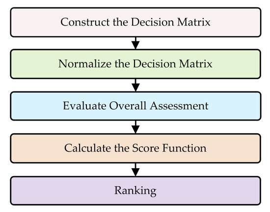
Figure 1.
Flowchart of the proposed algorithm.
6.1. Case Study
Electricity is a main energy resource among the different energy resources and has a high demand from the different economic sectors. Nevertheless, the production of electricity is followed by serious challenges of technology, climate, and sustainability. Fossil fuels such as coal, oil, and natural gas are the main primary energy resources used to generate electricity. It was recently reported that around 70% of electricity is produced worldwide from fossil fuels. Consequently, fossil fuel electricity generation also includes greenhouse gases (GHG), other emissions, and air pollutants. A comparison is made between coal, natural gas, nuclear, hydro, solar, wind, geothermal, and biomass generation. The parameters considered are system cost minimization, water footprint, and land intensity. The most popular energy modeling techniques include [144,145,146]:
- The energy and power evaluation program (ENPEP) is a nonlinear equilibrium model that balances the requirement for energy with available resources and technologies;
- Market allocation (MARKAL) is an integrated energy system that may be used to quantify the consequences of policy decisions on technology development and resource consumption;
- The model for the energy supply strategy alternatives and their general environmental impact (MESSAGE) combines technologies and fuels and constructs energy chains, which allows mapping energy flows from resource extraction to energy services; and
- The long-range energy alternatives planning system (LEAP) assists in energy policy analysis, especially tracking energy consumption, production, and resource extraction. These strategies are well designed for various levels of energy management. Energy models include a reliable framework to check predictions by organizing massive amounts of data in an open manner that reflects a stable system.
Across its background, Pakistan has suffered terrible energy challenges. The country’s energy crises, which extend mostly over a decade, have resulted in the collapse of thousands of factories, decreasing industrial production and influencing the lives of millions of families. For a developing country like Pakistan, choosing the best future direction of electricity generation is an inevitable challenge. In this context, energy modeling could be of great help if it takes into account the energy resource efficiency and the techno-economic and other relevant parameters to identify potential future energy pathways. Throughout the last quarter century, these crises have negatively affected the economy, with a loss of around 10% of the total gross domestic product(GDP). If not resolved at both the operational and strategic levels, Pakistan’s energy challenges could become a national interest threat [147].
In this analysis, electricity demand for the 2015–2050 time frame was calculated using the LEAP model. LEAP has become a consumer-friendly energy management tool that is used internationally for energy policy analysis. LEAP promotes a modeling approach based on scenarios by monitoring the growth, transition, and use of energy resources across the economy [148]. LEAP is a commonly used software tool developed at the Swedish Environment Institute for energy policy research and evaluation of climate change mitigation. LEAP has been implemented in far more than 190 countries around the world. The customers include state agencies, researchers, NGOs, consulting firms, and energy providers. It has been used from cities and countries to regional, national, and international applications in a wide range of dimensions. [149] When designing the modeling structure for Pakistan’s LEAP, 2015 was set as the reference year, as well 2050 as the final year. Reference (REF), which is an energy mechanism according to the latest plans and policies of the GOP, was the first supply side example. The paths of renewable energy technologies (RET) envisaged full penetration of renewable energy sources, and the scenario of clean coal maximum (CCM) foresees the use of reliable technologies for coal based power generation. The fourth scenario is called the energy efficiency and conservation (EEC) scenario. Pakistan’s total electricity requirement in 2050 is expected to be 1706.1 TWh, and in 2015, it was just 90.4 TWh. Because the REF, RET, and CCM scenarios were based on common demand-side assumptions, there was the same demand forecast for these three scenarios. For the EEC scenario, however, the projection of electricity demand for the same duration was calculated at 1373.2 TWh, which was 20 percent lower than the demand projected in the reference scenario.
Table 1 shows a concise overview of the main scenarios (alternatives).

Table 1.
Concise overview of the main scenarios. CCM, clean coal maximum; EEC, energy efficiency and conservation; RET, renewable energy technologies.
The supply side scenario alternatives were developed in the LEAP model in accordance with the different production technology’s resource potential and technical-economic parameters. The 2015/2050 generation (TWh) and installed power (GW) forecasts for various fuels and technologies are available. The total installed capacity in 2015 was 23.62 (GW). In 2015, the most widely used technology was oil and open cycle gas, which accounted for half of the installed capacity. Figure 2 presents installed capacity with respect to various fuels and technologies.
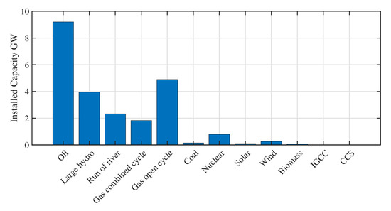
Figure 2.
Installed capacity with respect to various fuels and technologies for Pakistan (2015).
By the LEAP model, installed capacity by the different scenarios in 2050 was 425.94 (GW) by REF, 463.9 (GW) by RET, 416.21 (GW) by CCM, and 348.56 (GW) by EEC. Figure 3 shows installed capacity in different scenarios. The considered scenarios assumed a move away from oil processing and an increase in the share of renewable energy sources and increased use of coal.
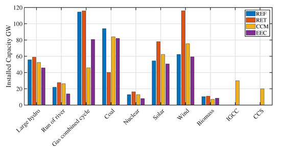
Figure 3.
Installed capacity in different scenarios for Pakistan (2050).
Generation was 108.3 (TWh) from various fuels and innovations in 2015. Figure 4 presents the details, where most of the electricity was generated using oil and hydro technologies. In this area, technologies related to coal, solar PV, lifts, and biomass were marginal.
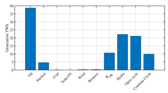
Figure 4.
Generation with respect to various fuels and technology in 2015.
Through LEAP, model generation in 2050 will be 1373.2 (TWh) and through EEC, 1706.10 (TWh) by REF, RET, and CCM across different scenarios. Figure 5 presents the generation in various scenarios for Pakistan in 2050. Renewable energy, such as run of river, biomass, and wind, will have the largest share in electricity generation with varying degrees depending on the chosen scenario.
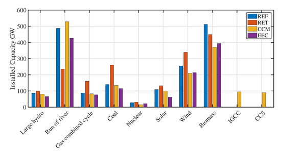
Figure 5.
Generation in different scenarios for Pakistan (2050).
To determine the best alternative among the four scenarios given in Table 1, we have the following criteria given in Table 2, which were selected on the basis of a literature review.
Table 2.
Criteria for evaluating the best alternative.
6.2. Illustrative Example
An illustrative example of the sustainable energy policy in Pakistan is given to illustrate the approach. Here, the set of alternatives is where = CCM, = EEC, = REF, and = RET. In evaluating these alternatives, we have the set of criteria given in Table 2 and take . Let be their corresponding weight vector, and assume that the expert provides his/her own point of view in the form of the decision matrix of the q-RONs as follows.
First, we get the normalized decision matrix by taking the compliment of the cost-type criteria, in Table 2 = land requirement, CO emission, = risk, and = investment cost are the cost-type criteria. is obtained by taking the compliment operation as follows.
Determine the cumulative assessments of the alternatives by using the q-ROFEWA operator.
For :
For :
For :
For :
Now, the values of the score related to each scenario are:
Now, rate the aggregate collective preferred value of using the score function in descending order. Figure 6 presents their comparison. corresponds to . Therefore, is the desired scenario. Strategies for productivity and capacity for recycling were considered under this scenario. The second place was taken by the scenario assuming sources of renewable energy of hydro, solar, wind, and biomass. The last position was taken by a scenario related to indigenous coal, oil, gas, and nuclear.
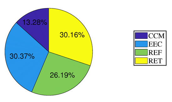
Figure 6.
Visualization of the relative assessment of the considered energy scenarios for Pakistan.
7. Conclusions
Proper mapping of uncertainty data and decision makers’ preferences is one of the biggest challenges in interdisciplinary research. MCDM has been applied widely to solve a number of real-world problems that involve impreciseness, uncertainty, and vagueness in the data. We focused on information aggregation for MCDM based on Yager’s q-ROFS model as this model is more practical and useful than the existing Yager’s Pythagorean fuzzy model and Atanassov’s intuitionistic fuzzy model. The decision makers can easily choose membership and non-membership grades from the alternatives in a larger space with the q-rung orthopair fuzzy set model. Most arithmetic tools rely on the min-max value of the observation set, while aggregation operators are mathematical tools that play an important role in converting a set of observations into a unique aggregated value. Hence, using all of these concepts, we introduced several new aggregation operators, namely the q-rung orthopair fuzzy Einstein weighted averaging (q-ROFEWA) operator, the q-rung orthopair fuzzy Einstein ordered weighted averaging (q-ROFEOWA) operator, the q-rung orthopair fuzzy Einstein weighted geometric (q-ROFEWG) operator, and the q-rung orthopair fuzzy Einstein ordered weighted geometric (q-ROFEOWG) operator under the q-ROF information. Some interesting features of the proposed operators were discussed, and their illustration was also given. A brief introduction about the t-norm and t-conorm was described, and new the t-norm and t-conorm for q-ROFNs were established. Finally, a numerical example of the proposed approach was cited to demonstrate the practical application of integrated energy modeling and sustainable energy planning issues. This research lays the groundwork for comprehensive energy planning studies in Pakistan by combining energy modeling and decision support as a common sustainable energy planning policy formulation process. We hope our findings will be fruitful for the researchers working in the fields of information aggregation, decision support systems, engineering, image processing, artificial intelligence, and medical diagnosis. Long-term work will pay special attention to interval-valued q-ROF Einstein aggregation operators, hesitant q-ROF Einstein fuzzy aggregation operators, and q-ROF m-polar Einstein fuzzy aggregation operators.
During the research, some possible areas of improvement of the proposed approach and future work directions were identified. When analyzing the formal basis of Yager’s q-rung orthopair fuzzy sets, it would be interesting to take into account their consistency. Afterward, extensive comparative studies of the authors’ approach with other fuzzy MCDM methods are suggested, covering not only the order of result ranking variants, but also accuracy, uncertainty level, and so on. Another potential direction of the development of the proposed method is reusable reference model building, including a full and coherent set of assessment criteria in the problem of sustainable energy planning, which for other researchers would be an important element of the model objectification for this complex decision making problem, but also of the proposed method’s effectiveness studies.
Author Contributions
This paper is a result of the common work of the authors in all aspects. All authors read and agreed to the published version of the manuscript.
Funding
The work was supported by the National Science Centre, Decision No. 2016/23/N/HS4/01931 (W.S.) and by the project financed within the framework of the program of the Minister of Science and Higher Education under the name “Regional Excellence Initiative” in the years 2019-2022, Project Number 001/RID/2018/19; the amount of financing: PLN 10.684.000,00 (J.W.).
Acknowledgments
The authors would like to thank the Editor and the anonymous reviewers, whose insightful comments and constructive suggestions helped us significantly improve the quality of this paper.
Conflicts of Interest
The authors declare no conflict of interest.
Abbreviations
The following abbreviations are used in this manuscript:
| REF | The current proposal and policy of the state is being pursued in this situation. |
| RET | Sustainable energy options and technology are favored under this situation. |
| CCM | The choice of clean coal is favorable under this scenario. |
| EEC | The efficiency and conservation measures are considered under this scenario. |
Appendix A
Appendix A.1.
Proof.
Here, we prove Theorem 3; (i), (iii), (iv), and (viii), are similar.
If we take:
Similarly:
Therefore, we write equivalent to:
Assume , , , and , then:
Now, suppose , , , , , , , . On the right-hand side,
Now,
Hence, it is proven.
Therefore, we write equivalent to:
Assume , , , and , then:
Now, suppose , , , , , , , . On the right-hand side,
Now,
Hence, it is proven.
Take :
where , , , . Therefore,
Hence, it is proven.
□
Appendix A.2.
Proof.
Theorem 3 is proven using mathematical induction.
For
As we know, both and are q-ROFNs, and also, is q-ROFN.
Then:
which proves this for .
Assume that the result is true for . We have:
Now, we will prove for ,
Thus, the result holds for . This proves the required result. □
Appendix A.3.
Proof.
(Theorem 4) Suppose is the family of q-ROFNs. By the Definition of q-ROFN,
Therefore,
and:
Therefore, we get .
For , we have:
Furthermore,
Moreover,
Hence, it is proven. □
Appendix A.4.
Proof.
(Theorem 5) Let and ; by Equation (3) we have:
This implies that
These are equal iff . Furthermore,
This implies that:
These are equal iff .
This implies:
Thus, we have the following relationship by defining the score function of q-ROFS.
□
Appendix A.5.
Proof.
We use mathematical induction to prove Theorem 11.
For :
As we know, both and are q-ROFNs, and also, is q-ROFN.
Then:
We proved this for .
Assume that the result for is true; we have:
Now, we will prove for ,
:
Thus, the result holds for . This proves the required result. □
Appendix A.6.
Proof.
Suppose is the family of q-ROFNs. By the definition of q-ROFN,
Therefore,
and:
Therefore, we get .
For , we have:
Furthermore,
Moreover,
Hence, it is proven. □
References
- Kaya, İ.; Çolak, M.; Terzi, F. A comprehensive review of fuzzy multi criteria decision making methodologies for energy policy making. Energy Strateg. Rev. 2019, 24, 207–228. [Google Scholar] [CrossRef]
- Çolak, M.; Kaya, İ. Prioritization of renewable energy alternatives by using an integrated fuzzy MCDM model: A real case application for Turkey. Renew. Sustain. Energy Rev. 2017, 80, 840–853. [Google Scholar] [CrossRef]
- Doukas, H.; Patlitzianas, K.D.; Psarras, J. Supporting sustainable electricity technologies in Greece using MCDM. Resour. Policy 2006, 31, 129–136. [Google Scholar] [CrossRef]
- Roy, B. Paradigms and challenges. In Multiple Criteria Decision Analysis: State of the Art Surveys; Springer: New York, NY, USA, 2005; pp. 3–24. [Google Scholar]
- Wang, J.J.; Jing, Y.Y.; Zhang, C.F.; Zhao, J.H. Review on multi-criteria decision analysis aid in sustainable energy decision making. Renew. Sustain. Energy Rev. 2009, 13, 2263–2278. [Google Scholar] [CrossRef]
- Faizi, S.; Sałabun, W.; Rashid, T.; Wątróbski, J.; Zafar, S. Group decision making for hesitant fuzzy sets based on characteristic objects method. Symmetry 2017, 9, 136. [Google Scholar] [CrossRef]
- Schläfke, M.; Silvi, R.; Möller, K. A framework for business analytics in performance management. Int. J. Product. Perform. Manag. 2013, 62, 110–122. [Google Scholar] [CrossRef]
- Faizi, S.; Rashid, T.; Sałabun, W.; Zafar, S.; Wątróbski, J. Decision making with uncertainty using hesitant fuzzy sets. Int. J. Fuzzy Syst. 2018, 20, 93–103. [Google Scholar] [CrossRef]
- Faizi, S.; Sałabun, W.; Ullah, S.; Rashid, T.; Więckowski, J. A New Method to Support Decision-Making in an Uncertain Environment Based on Normalized Interval-Valued Triangular Fuzzy Numbers and COMET Technique. Symmetry 2020, 12, 516. [Google Scholar] [CrossRef]
- Mardani, A.; Jusoh, A.; Zavadskas, E.K. Fuzzy multiple criteria decision making techniques and applications–Two decades review from 1994 to 2014. Expert Syst. Appl. 2015, 42, 4126–4148. [Google Scholar] [CrossRef]
- Corrente, S.; Figueira, J.R.; Greco, S.; Słowiński, R. A robust ranking method extending ELECTRE III to hierarchy of interacting criteria, imprecise weights and stochastic analysis. Omega 2017, 73, 1–17. [Google Scholar] [CrossRef]
- Wątróbski, J.; Jankowski, J.; Ziemba, P.; Karczmarczyk, A.; Zioło, M. Generalised framework for multi-criteria method selection. Omega 2019, 86, 107–124. [Google Scholar] [CrossRef]
- Mirakyan, A.; De Guio, R. Integrated energy planning in cities and territories: A review of methods and tools. Renew. Sustain. Energy Rev. 2013, 22, 289–297. [Google Scholar] [CrossRef]
- Strantzali, E.; Aravossis, K. Decision making in renewable energy investments: A review. Renew. Sustain. Energy Rev. 2016, 55, 885–898. [Google Scholar] [CrossRef]
- Løken, E. Use of multicriteria decision analysis methods for energy planning problems. Renew. Sustain. Energy Rev. 2007, 11, 1584–1595. [Google Scholar] [CrossRef]
- Martín-Gamboa, M.; Iribarren, D.; García-Gusano, D.; Dufour, J. A review of life-cycle approaches coupled with data envelopment analysis within multi-criteria decision analysis for sustainability assessment of energy systems. J. Clean. Prod. 2017, 150, 164–174. [Google Scholar] [CrossRef]
- Arce, M.E.; Saavedra, Á.; Míguez, J.L.; Granada, E. The use of grey-based methods in multi-criteria decision analysis for the evaluation of sustainable energy systems: A review. Renew. Sustain. Energy Rev. 2015, 47, 924–932. [Google Scholar] [CrossRef]
- Doukas, H. Modelling of linguistic variables in multicriteria energy policy support. Eur. J. Oper. Res. 2013, 227, 227–238. [Google Scholar] [CrossRef]
- Sałabun, W.; Piegat, A. Comparative analysis of MCDM methods for the assessment of mortality in patients with acute coronary syndrome. Artif. Intell. Rev. 2017, 48, 557–571. [Google Scholar] [CrossRef]
- Ribeiro, R.A. Fuzzy multiple attribute decision making: A review and new preference elicitation techniques. Fuzzy Sets Syst. 1996, 78, 155–181. [Google Scholar] [CrossRef]
- Sałabun, W.; Karczmarczyk, A.; Wątróbski, J.; Jankowski, J. Handling Data Uncertainty in Decision Making with COMET. In Proceedings of the 2018 IEEE Symposium Series on Computational Intelligence (SSCI), Bangalore, India, 18–21 Novermber 2018; pp. 1478–1484. [Google Scholar]
- Tecle, A. Choice of Multicriterion Decision Making Techniques for Watershed Management; The University of Arizona: Tucson, AZ, USA, 1988. [Google Scholar]
- Haimes, Y.Y.; Hall, W.A. Multiobjectives in water resource systems analysis: The surrogate worth trade off method. Water Resourc. Res. 1974, 10, 615–624. [Google Scholar] [CrossRef]
- Gershon, M.; Duckstein, L. A procedure for selection of a multiobjective technique with application to water and mineral resources. Appl. Math. Comput. 1984, 14, 245–271. [Google Scholar] [CrossRef]
- Tecle, A.; Fogel, M. Multiobjective wastewater management planning in a semiarid region. Ariz.-Nev. Acad. Sci. 1986, 16, 43–61. [Google Scholar]
- Ghandforoush, P.; Greber, B.J. Solving allocation and scheduling problems inherent in forest resource management using mixed-integer programming. Comput. Oper. Res. 1986, 13, 551–562. [Google Scholar] [CrossRef]
- Duckstein, L.; Gershon, M.; McAniff, R. Model selection in multiobjective decision making for river basin planning. Adv. Water Resour. 1982, 5, 178–184. [Google Scholar] [CrossRef]
- Romero, C.; Rehman, T. Natural resource management and the use of multiple criteria decision making techniques: A review. Eur. Rev. Agric. Econ. 1987, 14, 61–89. [Google Scholar] [CrossRef]
- Roy, B.; Hugonnard, J.C. Ranking of suburban line extension projects on the Paris metro system by a multicriteria method. Transp. Res. Part A Gen. 1982, 16, 301–312. [Google Scholar] [CrossRef]
- Nijkamp, P.; Spronk, J. Interactive multidimensional programming models for locational decisions. Eur. J. Oper. Res. 1981, 6, 220–223. [Google Scholar] [CrossRef]
- Werczberger, E. A goal-programming model for industrial location involving environmental considerations. Environ. Plan. A 1976, 8, 173–188. [Google Scholar] [CrossRef]
- Vachnadze, R.; Markozashvili, N. Some applications of the analytic hierarchy process. Math. Model. 1987, 9, 185–191. [Google Scholar] [CrossRef]
- Nijkamp, P.; Van Der Burch, M.; Vindigni, G. A comparative institutional evaluation of public-private partnerships in Dutch urban land-use and revitalisation projects. Urban Stud. 2002, 39, 1865–1880. [Google Scholar] [CrossRef]
- Ellis, H.M.; Keeney, R.L. A Rational Approach to Governmental Decision Concerning Air Pollution; Massachusetts Institute of Technology: Cambridge, MA, USA, 1971. [Google Scholar]
- Nijkamp, P.; van Delft, A. Multi-Criteria Analysis and Regional Decision-Making; Springer Science & Business Media: Berlin, Germany, 1977; Volume 8. [Google Scholar]
- Punj, G.N.; Staelin, R. The choice process for graduate business schools. J. Mark. Res. 1978, 15, 588–598. [Google Scholar] [CrossRef]
- Bouyssou, D. Building criteria: A prerequisite for MCDA. In Readings in Multiple Criteria Decision Aid; Springer: Berlin/Heidelberg, Germany, 1990; pp. 58–80. [Google Scholar]
- Keeney, R.L.; Raiffa, H. Decision Analysis with Multiple Conflicting Objectives; Wiley& Sons: New York, NY, USA, 1976. [Google Scholar]
- Siskos, J.; Zopounidis, C. The evaluation criteria of the venture capital investment activity: An interactive assessment. Eur. J. Oper. Res. 1987, 31, 304–313. [Google Scholar] [CrossRef]
- Nijkamp, P.; Spronk, J. Multiple Criteria Analysis: Operational Methods; Lexington Books: Plymouth, UK, 1981. [Google Scholar]
- Duckstein, L. Multiobjective Optimization in Structural Design: The Model Choice Problem; Technical Report; Arizona Univ Tucson Dept of Systems and Industrial Engineering: Tucson, AZ, USA, 1981. [Google Scholar]
- Despontin, M.; Vincke, P. Multiple Criteria Economic Policy; Advances in Operations Research; North-Holland Publ. Co.: Amsterdam, The Netherlands, 1977. [Google Scholar]
- Herner, S.; Snapper, K.J. The application of multiple-criteria utility theory to the evaluation of information systems. J. Am. Soc. Inf. Sci. 1978, 29, 289–296. [Google Scholar] [CrossRef]
- MacCrimmon, K.R. Decisionmaking among Multiple-Attribute Alternatives: A Survey and Consolidated Approach; Technical Report; Rand Corp.: Santa Monica, CA, USA, 1968. [Google Scholar]
- Labuschagne, C.; Brent, A.C.; Van Erck, R.P. Assessing the sustainability performances of industries. J. Clean. Prod. 2005, 13, 373–385. [Google Scholar] [CrossRef]
- Janssen, R. Multiobjective Decision Support for Environmental Management; Springer Science & Business Media: Berlin, Germany, 2012; Volume 2. [Google Scholar]
- Sala, S.; Ciuffo, B.; Nijkamp, P. A systemic framework for sustainability assessment. Ecol. Econ. 2015, 119, 314–325. [Google Scholar] [CrossRef]
- Awan, M.A.; Ali, Y. Sustainable modeling in reverse logistics strategies using fuzzy MCDM. Manag. Environ. Qual. Int. J. 2019, 30, 1132–1151. [Google Scholar] [CrossRef]
- Boggia, A.; Cortina, C. Measuring sustainable development using a multi-criteria model: A case study. J. Environ. Manag. 2010, 91, 2301–2306. [Google Scholar] [CrossRef]
- Ishizaka, A.; Labib, A. Analytic hierarchy process and expert choice: Benefits and limitations. Or Insight 2009, 22, 201–220. [Google Scholar] [CrossRef]
- Shahroodi, K.; Amin, K.; Shabnam, A.; Elnaz, S.; Najibzadeh, M. Application of analytical hierarchy process (AHP) technique to evaluate and selecting suppliers in an effective supply chain. Kuwait Chapter Arab. J. Bus. Manag. Rev. 2012, 33, 1–14. [Google Scholar]
- Edwards, W.; Newman, J.R.; Snapper, K.; Seaver, D. Multiattribute Evaluation; Number 26; Chronicle Books: San Francisco, CA, USA, 1982. [Google Scholar]
- Wang, J.; Zionts, S. Negotiating wisely: Considerations based on MCDM/MAUT. Eur. J. Oper. Res. 2008, 188, 191–205. [Google Scholar] [CrossRef]
- Wątróbski, J.; Ziemba, E.; Karczmarczyk, A.; Jankowski, J. An index to measure the sustainable information society: The Polish households case. Sustainability 2018, 10, 3223. [Google Scholar] [CrossRef]
- Al-Shalabi, M.A.; Mansor, S.B.; Ahmed, N.B.; Shiriff, R. GIS based multicriteria approaches to housing site suitability assessment. In Proceedings of the XXIII FIG Congress, Shaping the Change, Munich, Germany, 8–13 October 2006; pp. 8–13. [Google Scholar]
- Liu, H.C.; Mao, L.X.; Zhang, Z.Y.; Li, P. Induced aggregation operators in the VIKOR method and its application in material selection. Appl. Math. Model. 2013, 37, 6325–6338. [Google Scholar] [CrossRef]
- Kwak, N.; Lee, C.W.; Kim, J.H. An MCDM model for media selection in the dual consumer/industrial market. Eur. J. Oper. Res. 2005, 166, 255–265. [Google Scholar] [CrossRef]
- Yue, W.; Cai, Y.; Rong, Q.; Cao, L.; Wang, X. A hybrid MCDA-LCA approach for assessing carbon foot-prints and environmental impacts of China’s paper producing industry and printing services. Environ. Syst. Res. 2014, 3, 4. [Google Scholar] [CrossRef]
- Koschke, L.; Fürst, C.; Frank, S.; Makeschin, F. A multi-criteria approach for an integrated land-cover-based assessment of ecosystem services provision to support landscape planning. Ecol. Indic. 2012, 21, 54–66. [Google Scholar] [CrossRef]
- Jankowski, J.; Hamari, J.; Wątróbski, J. A gradual approach for maximizing user conversion without compromising experience with high visual intensity website elements. arXiv 2019, arXiv:1903.11997. [Google Scholar]
- Samal, R.K.; Kansal, M.L. Sustainable development contribution assessment of renewable energy projects using AHP and compromise programming techniques. In Proceedings of the 2015 International Conference on Energy, Power and Environment: Towards Sustainable Growth (ICEPE), Shillong, India, 12–13 June 2015; pp. 1–6. [Google Scholar]
- Govindan, K.; Jepsen, M.B. ELECTRE: A comprehensive literature review on methodologies and applications. Eur. J. Oper. Res. 2016, 250, 1–29. [Google Scholar] [CrossRef]
- Hatefi, S.; Torabi, S. A slack analysis framework for improving composite indicators with applications to human development and sustainable energy indices. Econ. Rev. 2018, 37, 247–259. [Google Scholar] [CrossRef]
- Linhoss, A.; Jeff Ballweber, J. Incorporating uncertainty and decision analysis into a water-sustainability index. J. Water Resour. Plan. Manag. 2015, 141, A4015007. [Google Scholar] [CrossRef]
- Cucchiella, F.; D’Adamo, I.; Gastaldi, M.; Koh, S.L.; Rosa, P. A comparison of environmental and energetic performance of European countries: A sustainability index. Renew. Sustain. Energy Rev. 2017, 78, 401–413. [Google Scholar] [CrossRef]
- Kumar, T.; Jhariya, D. Land quality index assessment for agricultural purpose using multi-criteria decision analysis (MCDA). Geocarto Int. 2015, 30, 822–841. [Google Scholar] [CrossRef]
- Sałabun, W.; Wątróbski, J.; Piegat, A. Identification of a multi-criteria model of location assessment for renewable energy sources. In International Conference on Artificial Intelligence and Soft Computing; Springer: Cham, Switzerland, 2016; pp. 321–332. [Google Scholar]
- Pohekar, S.; Ramachandran, M. Application of multi-criteria decision making to sustainable energy planning—A review. Renew. Sustain. Energy Rev. 2004, 8, 365–381. [Google Scholar] [CrossRef]
- Ilbahar, E.; Cebi, S.; Kahraman, C. A state-of-the-art review on multi-attribute renewable energy decision making. Energy Strateg. Rev. 2019, 25, 18–33. [Google Scholar] [CrossRef]
- Roy, B. Multicriteria Methodology for Decision Aiding; Springer Science & Business Media: Berlin, Germany, 2013; Volume 12. [Google Scholar]
- Zyoud, S.H.; Fuchs-Hanusch, D. A bibliometric-based survey on AHP and TOPSIS techniques. Expert Syst. Appl. 2017, 78, 158–181. [Google Scholar] [CrossRef]
- Ahmad, S.; Tahar, R.M. Selection of renewable energy sources for sustainable development of electricity generation system using analytic hierarchy process: A case of Malaysia. Renew. Energy 2014, 63, 458–466. [Google Scholar] [CrossRef]
- Wang, Y.; Xu, L.; Solangi, Y.A. Strategic renewable energy resources selection for Pakistan: Based on SWOT-Fuzzy AHP approach. Sustain. Cities Soc. 2020, 52, 101861. [Google Scholar] [CrossRef]
- Erol, Ö.; Kılkış, B. An energy source policy assessment using analytical hierarchy process. Energy Convers. Manag. 2012, 63, 245–252. [Google Scholar] [CrossRef]
- Abdullah, L.; Najib, L. Sustainable energy planning decision using the intuitionistic fuzzy analytic hierarchy process: Choosing energy technology in Malaysia. Int. J. Sustain. Energy 2016, 35, 360–377. [Google Scholar] [CrossRef]
- Vavrek, R.; Chovancová, J. Assessment of economic and environmental energy performance of EU countries using CV-TOPSIS technique. Ecol. Indic. 2019, 106, 105519. [Google Scholar] [CrossRef]
- Mojaver, P.; Khalilarya, S.; Chitsaz, A.; Assadi, M. Multi-objective optimization of a power generation system based SOFC using Taguchi/AHP/TOPSIS triple method. Sustain. Energy Technol. Assess. 2020, 38, 100674. [Google Scholar] [CrossRef]
- Liu, J.; Yin, Y. An integrated method for sustainable energy storing node optimization selection in China. Energy Convers. Manag. 2019, 199, 112049. [Google Scholar] [CrossRef]
- Wang, B.; Song, J.; Ren, J.; Li, K.; Duan, H. Selecting sustainable energy conversion technologies for agricultural residues: A fuzzy AHP-VIKOR based prioritization from life cycle perspective. Resour. Conserv. Recycl. 2019, 142, 78–87. [Google Scholar] [CrossRef]
- Ziemba, P.; Wątróbski, J.; Zioło, M.; Karczmarczyk, A. Using the PROSA method in offshore wind farm location problems. Energies 2017, 10, 1755. [Google Scholar] [CrossRef]
- Ziemba, P. Towards strong sustainability management—A generalized PROSA method. Sustainability 2019, 11, 1555. [Google Scholar] [CrossRef]
- Bhowmik, C.; Bhowmik, S.; Ray, A.; Pandey, K.M. Optimal green energy planning for sustainable development: A review. Renew. Sustain. Energy Rev. 2017, 71, 796–813. [Google Scholar] [CrossRef]
- Mousavi, M.; Gitinavard, H.; Mousavi, S. A soft computing based-modified ELECTRE model for renewable energy policy selection with unknown information. Renew. Sustain. Energy Rev. 2017, 68, 774–787. [Google Scholar] [CrossRef]
- Schröder, T.; Lauven, L.P.; Beyer, B.; Lerche, N.; Geldermann, J. Using PROMETHEE to assess bioenergy pathways. Cent. Eur. J. Oper. Res. 2019, 27, 287–309. [Google Scholar] [CrossRef]
- Tabaraee, E.; Ebrahimnejad, S.; Bamdad, S. Evaluation of power plants to prioritise the investment projects using fuzzy PROMETHEE method. Int. J. Sustain. Energy 2018, 37, 941–955. [Google Scholar] [CrossRef]
- Sharma, D.; Pandey, A.; Kumar, C.; Ranjan, R. Assessment & anthology of sustainable sources of energy using an approach of PROMETHEE. In IOP Conference Series: Materials Science and Engineering; IOP Publishing: Bristol, UK, 2019; Volume 691, p. 012040. [Google Scholar]
- Dias, L.C.; Antunes, C.H.; Dantas, G.; de Castro, N.; Zamboni, L. A multi-criteria approach to sort and rank policies based on Delphi qualitative assessments and ELECTRE TRI: The case of smart grids in Brazil. Omega 2018, 76, 100–111. [Google Scholar] [CrossRef]
- Peng, H.G.; Shen, K.W.; He, S.S.; Zhang, H.Y.; Wang, J.Q. Investment risk evaluation for new energy resources: An integrated decision support model based on regret theory and ELECTRE III. Energy Convers. Manag. 2019, 183, 332–348. [Google Scholar] [CrossRef]
- Özcan, E.C.; Ünlüsoy, S.; Eren, T. A combined goal programming–AHP approach supported with TOPSIS for maintenance strategy selection in hydroelectric power plants. Renew. Sustain. Energy Rev. 2017, 78, 1410–1423. [Google Scholar] [CrossRef]
- Kaya, T.; Kahraman, C. Multicriteria renewable energy planning using an integrated fuzzy VIKOR & AHP methodology: The case of Istanbul. Energy 2010, 35, 2517–2527. [Google Scholar]
- Solangi, Y.A.; Tan, Q.; Mirjat, N.H.; Ali, S. Evaluating the strategies for sustainable energy planning in Pakistan: An integrated SWOT-AHP and Fuzzy-TOPSIS approach. J. Clean. Prod. 2019, 236, 117655. [Google Scholar] [CrossRef]
- Zadeh, L.A. Fuzzy sets. Inf. Control 1965, 8, 338–353. [Google Scholar] [CrossRef]
- Atanassov, K.T. More on intuitionistic fuzzy sets. Fuzzy Sets Syst. 1989, 33, 37–45. [Google Scholar] [CrossRef]
- Yager, R.R. Pythagorean fuzzy subsets. In Proceedings of the 2013 joint IFSA world congress and NAFIPS annual meeting (IFSA/NAFIPS), Edmonton, AB, Canada, 24–28 June 2013; pp. 57–61. [Google Scholar]
- Yager, R.R.; Abbasov, A.M. Pythagorean membership grades, complex numbers, and decision making. Int. J. Intell. Syst. 2013, 28, 436–452. [Google Scholar] [CrossRef]
- Yager, R.R. Pythagorean membership grades in multicriteria decision making. IEEE Trans. Fuzzy Syst. 2013, 22, 958–965. [Google Scholar] [CrossRef]
- Bashir, Z.; Rashid, T.; Sałabun, W.; Zafar, S. Certain convergences for intuitionistic fuzzy sets. J. Intell. Fuzzy Syst. 2020, 38, 553–564. [Google Scholar] [CrossRef]
- Yager, R.R. Generalized orthopair fuzzy sets. IEEE Trans. Fuzzy Syst. 2016, 25, 1222–1230. [Google Scholar] [CrossRef]
- Yager, R.R. On ordered weighted averaging aggregation operators in multicriteria decisionmaking. IEEE Trans. Syst. Man Cybern. 1988, 18, 183–190. [Google Scholar] [CrossRef]
- Akram, M. Bipolar fuzzy graphs. Inf. Sci. 2011, 181, 5548–5564. [Google Scholar] [CrossRef]
- Akram, M.; Ali, G.; Alshehri, N.O. A new multi-attribute decision making method based on m-polar fuzzy soft rough sets. Symmetry 2017, 9, 271. [Google Scholar] [CrossRef]
- Akram, M.; Sayed, S.; Smarandache, F. Neutrosophic incidence graphs with application. Axioms 2018, 7, 47. [Google Scholar] [CrossRef]
- Akram, M.; Waseem, N.; Liu, P. Novel Approach in Decision Making with m—Polar Fuzzy ELECTRE-I. Int. J. Fuzzy Syst. 2019, 21, 1117–1129. [Google Scholar] [CrossRef]
- Ali, M.I. A note on soft sets, rough soft sets and fuzzy soft sets. Appl. Soft Comput. 2011, 11, 3329–3332. [Google Scholar]
- Garg, H.; Arora, R. Generalized intuitionistic fuzzy soft power aggregation operator based on t-norm and their application in multicriteria decision making. Int. J. Intell. Syst. 2019, 34, 215–246. [Google Scholar] [CrossRef]
- Garg, H.; Arora, R. Dual hesitant fuzzy soft aggregation operators and their application in decision making. Cogn. Comput. 2018, 10, 769–789. [Google Scholar] [CrossRef]
- Garg, H.; Arora, R. A nonlinear-programming methodology for multi-attribute decision making problem with interval-valued intuitionistic fuzzy soft sets information. Appl. Intell. 2018, 48, 2031–2046. [Google Scholar] [CrossRef]
- Garg, H.; Arora, R. Novel scaled prioritized intuitionistic fuzzy soft interaction averaging aggregation operators and their application to multi criteria decision making. Eng. Appl. Artif. Intell. 2018, 71, 100–112. [Google Scholar] [CrossRef]
- Hashmi, M.R.; Riaz, M.; Smarandache, F. m-polar Neutrosophic Topology with Applications to Multi-Criteria Decision-Making in Medical Diagnosis and Clustering Analysis. Int. J. Fuzzy Syst. 2020, 22, 273–292. [Google Scholar] [CrossRef]
- Hashmi, M.R.; Riaz, M. A novel approach to censuses process by using Pythagorean m-polar fuzzy Dombi’s aggregation operators. J. Intell. Fuzzy Syst. 2020, 38, 1977–1995. [Google Scholar] [CrossRef]
- Kumar, K.; Garg, H. TOPSIS method based on the connection number of set pair analysis under interval-valued intuitionistic fuzzy set environment. Comput. Appl. Math. 2018, 37, 1319–1329. [Google Scholar] [CrossRef]
- Karaaslan, F. Neutrosophic soft sets with applications in decision making. Int. J. Inf. Sci. Intell. Syst. 2015, 2, 1–20. [Google Scholar]
- Naeem, K.; Riaz, M.; Peng, X.; Afzal, D. Pythagorean fuzzy soft MCGDM methods based on TOPSIS, VIKOR and aggregation operators. J. Intell. Fuzzy Syst. 2019, 37, 6937–6957. [Google Scholar] [CrossRef]
- Naeem, K.; Riaz, M.; Afzal, D. Pythagorean m-polar fuzzy sets and TOPSIS method for the selection of advertisement mode. J. Intell. Fuzzy Syst. 2019, 37, 8441–8458. [Google Scholar] [CrossRef]
- Peng, X.; Yang, Y. Some results for Pythagorean fuzzy sets. Int. J. Intell. Syst. 2015, 30, 1133–1160. [Google Scholar] [CrossRef]
- Peng, X.; Yuan, H.; Yang, Y. Pythagorean fuzzy information measures and their applications. Int. J. Intell. Syst. 2017, 32, 991–1029. [Google Scholar] [CrossRef]
- Peng, X.; Selvachandran, G. Pythagorean fuzzy set: State of the art and future directions. Artif. Intell. Rev. 2019, 52, 1873–1927. [Google Scholar] [CrossRef]
- Peng, X.; Yang, Y.; Song, J.; Jiang, Y. Pythagorean fuzzy soft set and its application. Comput. Eng. 2015, 41, 224–229. [Google Scholar]
- Peng, X.; Dai, J. Approaches to single-valued neutrosophic MADM based on MABAC, TOPSIS and new similarity measure with score function. Neural Comput. Appl. 2018, 29, 939–954. [Google Scholar] [CrossRef]
- Riaz, M.; Çağman, N.; Zareef, I.; Aslam, M. N-soft topology and its applications to multi-criteria group decision making. J. Intell. Fuzzy Syst. 2019, 36, 6521–6536. [Google Scholar] [CrossRef]
- Riaz, M.; Smarandache, F.; Firdous, A.; Fakhar, A. On soft rough topology with multi-attribute group decision making. Mathematics 2019, 7, 67. [Google Scholar] [CrossRef]
- Riaz, M.; Davvaz, B.; Firdous, A.; Fakhar, A. Novel concepts of soft rough set topology with applications. J. Intell. Fuzzy Syst. 2019, 36, 3579–3590. [Google Scholar] [CrossRef]
- Riaz, M.; Hashmi, M.R. MAGDM for agribusiness in the environment of various cubic m-polar fuzzy averaging aggregation operators. J. Intell. Fuzzy Syst. 2019, 37, 3671–3691. [Google Scholar] [CrossRef]
- Riaz, M.; Hashmi, M.R. Linear Diophantine fuzzy set and its applications towards multi-attribute decision making problems. J. Intell. Fuzzy Syst. 2019, 37, 5417–5439. [Google Scholar] [CrossRef]
- Riaz, M.; Hashmi, M.R. Soft rough Pythagorean m-polar fuzzy sets and Pythagorean m-polar fuzzy soft rough sets with application to decision making. Comput. Appl. Math. 2020, 39, 16. [Google Scholar] [CrossRef]
- Riaz, M.; Tehrim, S.T. Certain properties of bipolar fuzzy soft topology via Q-neighborhood. Punjab Univ. J. Math. 2019, 51, 113–131. [Google Scholar]
- Riaz, M.; Tehrim, S.T. Cubic bipolar fuzzy ordered weighted geometric aggregation operators and their application using internal and external cubic bipolar fuzzy data. Comput. Appl. Math. 2019, 38, 87. [Google Scholar] [CrossRef]
- Riaz, M.; Tehrim, S.T. Multi-attribute group decision making based on cubic bipolar fuzzy information using averaging aggregation operators. J. Intell. Fuzzy Syst. 2019, 37, 2473–2494. [Google Scholar] [CrossRef]
- Riaz, M.; Tehrim, S.T. Bipolar fuzzy soft mappings with application to bipolar disorders. Int. J. Biomath. 2019, 12, 1950080. [Google Scholar] [CrossRef]
- Tehrim, S.T.; Riaz, M. A novel extension of TOPSIS to MCGDM with bipolar neutrosophic soft topology. J. Intell. Fuzzy Syst. 2019, 37, 5531–5549. [Google Scholar] [CrossRef]
- Xu, Z. Intuitionistic fuzzy aggregation operators. IEEE Trans. Fuzzy Syst. 2007, 15, 1179–1187. [Google Scholar]
- Xu, Z.; Cai, X. Intuitionistic Fuzzy Information Aggregation: Theory and Applications; Springer Science & Business Media: Berlin, Germany, 2013. [Google Scholar]
- Xu, Z. Hesitant Fuzzy Sets Theory; Springer: Cham, Switzerland, 2014; Volume 314. [Google Scholar]
- Ye, J. Interval-valued hesitant fuzzy prioritized weighted aggregation operators for multiple attribute decision making. J. Algorithms Comput. Technol. 2014, 8, 179–192. [Google Scholar] [CrossRef]
- Ye, J. Linguistic neutrosophic cubic numbers and their multiple attribute decision making method. Information 2017, 8, 110. [Google Scholar] [CrossRef]
- Zhan, J.; Liu, Q.; Davvaz, B. A new rough set theory: Rough soft hemirings. J. Intell. Fuzzy Syst. 2015, 28, 1687–1697. [Google Scholar] [CrossRef]
- Zhan, J.; Alcantud, J.C.R. A novel type of soft rough covering and its application to multicriteria group decision making. Artif. Intell. Rev. 2019, 52, 2381–2410. [Google Scholar] [CrossRef]
- Zhang, L.; Zhan, J. Fuzzy soft beta-covering based fuzzy rough sets and corresponding decision making applications. Int. J. Mach. Learn. Cybern. 2019, 10, 1487–1502. [Google Scholar] [CrossRef]
- Zhang, L.; Zhan, J.; Alcantud, J.C.R. Novel classes of fuzzy soft β-coverings based fuzzy rough sets with applications to multi-criteria fuzzy group decision making. Soft Comput. 2019, 23, 5327–5351. [Google Scholar] [CrossRef]
- Zhang, L.; Zhan, J.; Xu, Z. Covering-based generalized IF rough sets with applications to multi-attribute decision making. Inf. Sci. 2019, 478, 275–302. [Google Scholar] [CrossRef]
- Ali, M.I. Another view on q-rung orthopair fuzzy sets. Int. J. Intell. Syst. 2018, 33, 2139–2153. [Google Scholar] [CrossRef]
- Liu, P.; Wang, P. Some q-rung orthopair fuzzy aggregation operators and their applications to multiple-attribute decision making. Int. J. Intell. Syst. 2018, 33, 259–280. [Google Scholar] [CrossRef]
- Liu, Y.; Zhang, H.; Wu, Y.; Dong, Y. Ranking range based approach to MADM under incomplete context and its application in venture investment evaluation. Technol. Econ. Dev. Econ. 2019, 25, 877–899. [Google Scholar] [CrossRef]
- Phdungsilp, A.; Wuttipornpun, T. Analyses of the decarbonizing Thailand’s energy system toward low-carbon futures. Renew. Sustain. Energy Rev. 2013, 24, 187–197. [Google Scholar] [CrossRef]
- Mirjat, N.H.; Uqaili, M.A.; Harijan, K.; Valasai, G.D.; Shaikh, F.; Waris, M. A review of energy and power planning and policies of Pakistan. Renew. Sustain. Energy Rev. 2017, 79, 110–127. [Google Scholar] [CrossRef]
- Sahir, M.H. Energy System Modeling and Analysis of Long Term Sustainable Energy Alternatives for Pakistan. Ph.D. Thesis, University of Engineering and Technology Taxila-Pakistan, Taxila, Pakistan, 2007. [Google Scholar]
- Valasai, G.D.; Uqaili, M.A.; Memon, H.R.; Samoo, S.R.; Mirjat, N.H.; Harijan, K. Overcoming electricity crisis in Pakistan: A review of sustainable electricity options. Renew. Sustain. Energy Rev. 2017, 72, 734–745. [Google Scholar] [CrossRef]
- Heaps, C.G. Long-Range Energy Alternatives Planning (LEAP) System; Stockholm Environment Institute: Stockholm, Sweden, 2016. [Google Scholar]
- Hussain Mirjat, N.; Uqaili, M.A.; Harijan, K.; Mustafa, M.W.; Rahman, M.; Khan, M. Multi-criteria analysis of electricity generation scenarios for sustainable energy planning in Pakistan. Energies 2018, 11, 757. [Google Scholar] [CrossRef]
- Amer, M.; Daim, T.U. Selection of renewable energy technologies for a developing county: A case of Pakistan. Energy Sustain. Dev. 2011, 15, 420–435. [Google Scholar] [CrossRef]
- Balin, A.; Baraçli, H. A fuzzy multi-criteria decision making methodology based upon the interval type-2 fuzzy sets for evaluating renewable energy alternatives in Turkey. Technol. Econ. Dev. Econ. 2017, 23, 742–763. [Google Scholar] [CrossRef]
- Kahraman, C.; Cebi, S.; Kaya, I. Selection among renewable energy alternatives using fuzzy axiomatic design: The case of Turkey. J. UCS 2010, 16, 82–102. [Google Scholar]
- Kahraman, C.; Kaya, İ. A fuzzy multicriteria methodology for selection among energy alternatives. Expert Syst. Appl. 2010, 37, 6270–6281. [Google Scholar] [CrossRef]
- Kahraman, C.; Kaya, İ.; Cebi, S. A comparative analysis for multiattribute selection among renewable energy alternatives using fuzzy axiomatic design and fuzzy analytic hierarchy process. Energy 2009, 34, 1603–1616. [Google Scholar] [CrossRef]
- Ribeiro, F.; Ferreira, P.; Araújo, M. Evaluating future scenarios for the power generation sector using a Multi-Criteria Decision Analysis (MCDA) tool: The Portuguese case. Energy 2013, 52, 126–136. [Google Scholar] [CrossRef]
- Adhikary, P.; Roy, P.K.; Mazumdar, A. Multidimensional feasibility analysis of small hydropower project in India: A case study. ARPN J. Eng. Appl. Sci. 2014, 9, 80–84. [Google Scholar]
- Abu-Taha, R. Multi-criteria applications in renewable energy analysis: A literature review. In Proceedings of the 2011 Proceedings of PICMET’11: Technology Management in the Energy Smart World (PICMET), Portland, OR, USA, 31 July–4 August 2011; pp. 1–8. [Google Scholar]
- Kumar, A.; Sah, B.; Singh, A.R.; Deng, Y.; He, X.; Kumar, P.; Bansal, R. A review of multi criteria decision making (MCDM) towards sustainable renewable energy development. Renew. Sustain. Energy Rev. 2017, 69, 596–609. [Google Scholar] [CrossRef]
- Fleten, S.E.; Maribu, K.M.; Wangensteen, I. Optimal investment strategies in decentralized renewable power generation under uncertainty. Energy 2007, 32, 803–815. [Google Scholar] [CrossRef]


© 2020 by the authors. Licensee MDPI, Basel, Switzerland. This article is an open access article distributed under the terms and conditions of the Creative Commons Attribution (CC BY) license (http://creativecommons.org/licenses/by/4.0/).