1. Introduction
The point reactor is an important model when space variations are neglected. More realistic models should account for the stochastic variations due to nonlinearities and uncertainties due different sources. The startup random variations have considerable effect on the reactor power and should not be neglected. [
1] As a result, the thermal hydraulics in the reactor are affected by the power jumps that may cause thermal shocks to the mechanical elements. Robust controllers are required to manage the uncertainties and nonlinearities in the reactor to obtain the required performance for a range of different operating conditions [
2].
The stochastic point kinetic (SPK) reactor model can be analyzed with different techniques. The Monte-Carlo technique (MC) and the point collocation (PCA) technique are considered in [
3]. Taylor expansion technique with Euler-Maruyama (EM) are considered in [
4]. A simplified SPK model (SSPK), at which no square-root of a matrix is required, is deduced and used efficiently in the analysis [
5]. The main advantage of SSPK is avoiding the time-consuming computations of the covariance matrix square root. The Winer-Ito expansion (WIE) is used to analyze SSPK by separating the mean and higher-order moments and hence avoid using sampling techniques. Additionally, WIE is used to predict the startup transients in the neutronic power density [
1].
The heat produced in the nuclear reactor is transferred through heat exchangers for industrial utilization. Controlling the overall heat exchange is important to keep the reactor working at high efficiency. Heat exchange control with reactor is investigated in the literature. The efficiency of the fuzzy proportional-integral-derivative was examined and compared with the traditional controllers. The fractional order controllers are examined in [
2] and are found to perform better in most cases. Further improvements and more analysis considering the disturbances are considered in [
6]. A mathematical model that combines the deterministic point kinetics with the thermal hydraulics is developed in [
7].
The spectral stochastic techniques, based on Fourier-like decompositions, are used efficiently for analyzing the stochastic and/or random variations in the systems. The polynomial chaos expansion (PCE) and its generalized (gPC) version are efficiently used in case of random variation in the system parameters [
8]. The random variations are parameters with given probability distributions and hence the statistical properties, such as mean and variance, are known. In case of randomness due to noise, many techniques (e.g., EM and WIE) can be used [
9]. WIE has the advantage of having a high, sometimes exponential, rate of convergence.
In this work, a more practical point reactor model with both noise and uncertain parameters is considered. This will result in a more complicated model with different sources of uncertainties. A mixed spectral technique is proposed to analyze and quantify the uncertainties. The model is expanded with WIE to handle the noise, while the random parameters are handled with gPC. The statistical properties of both WIE and gPC are used to decompose the model into a deterministic system. The thermal hydraulics based on lumped parameter is analyzed. The classical analytical and/or numerical techniques can be used to solve the system and compute the statistics. Two test cases for stochastic point-reactor with six groups are considered to test the proposed technique and compare it with the traditional techniques.
The paper is organized as follows;
Section 2 summarizes the spectral stochastic and random techniques—WIE and gPC and their combination.
Section 3 explains the reactor model with the thermal equilibrium and the assumptions used in the analysis.
Section 4 explains the application of the hybrid expansion and the resulting deterministic system.
Section 5 introduces the results and the analysis.
2. Spectral Stochastic and Random Techniques
WIE is widely used as a spectral technique for analyzing stochastic processes with noise. Consider the second-order, finite-variance, stochastic process
, the
truncated WIE decomposition is written as [
10]:
The deterministic kernels are assumed, without loss of generality, to be symmetric in the variables . The basis function is the jth–order Hermite polynomial.
Using WIE results in an exact solution for the Gaussian processes. For the near Gaussian processes, the convergence of WIE will be exponential. The convergence rate will decrease in case of severe non-linearities and/or relatively large times. In this case, a time-dependent basis will be required [
11].
The gPC technique is efficiently used for processes with random parameters [
12]. Given the output
of a random experiment and consider the model parameters vector
that depends on a set of
random variables
of any known distribution. Consider the orthonormal basis
for the space
of second-order functionals. Then, any random process
in
is decomposed as:
Practically, the expansion is truncated up to
terms. The gPC representation is convergent in the mean-square sense. Proper selection of basis functions leads to a high rate, sometimes exponential, of convergence [
13].
The WIE and gPC can be combined to analyze systems with hybrid sources of uncertainties, noise and random parameters. In this case, the stochastic process is expanded as:
In case of independent noise and random parameters, the mean
and variance
are obtained as [
10]:
The individual contribution of each random source and the mixed contributions can be quantified by decomposing the variance. The variance formula (4) can be decomposed into three components; due to noise
, due to random parameters
, and due to mixed contributions
:
Using the decomposition (5), the system sensitivity indices [
14] due to different parameters can be easily obtained. For example, the sensitivity due to noise is evaluated as
.
3. The Point-Reactor Model with Stochastic Variations
The point-reactor model with stochastic variations (SPK) is derived by considering the probabilities of basic processes in the reactor that can occur in a small time interval. This will result in a system of Itô stochastic differential equations as [
3]:
With , , , , , .
Where is the reactor thermal (neutronic) power, is group delayed precursor density, is the rate of external neutron source, is the delayed neutron fraction, is the total reactivity, is the precursor group decay constant (per second), is the lifetime (sec) of prompt neutron, and is the fission average number of neutrons.
One of the computational difficulties of SPK model is the eigenvalue problem required to compute the covariance matrix square root. This time-consuming computations are evaluated each time step and hence will raise the complexity of the model. An alternative stochastic model is developed at which the square root is evaluated for each element of the matrix instead of the overall matrix as described in [
15].
A simplified SPK version (SSPK) of (6) is developed in [
5] by neglecting the mutual covariances between the neutron and precursor populations. In SSPK, the time-consuming eigenvalue problem is not required as ther is no matrix square-root. This will reduce dramatically the complexity of the SPK model (6).
The SSPK model can be written in terms of the thermal power
as [
5]:
where
. System (7) can be also written in terms of the average number of neutrons
(per m
3) by using the relation between the thermal/neutronic power
and the average neutron density
, where:
where
and
are the nominal (full power) thermal power and neutron density respectively.
The lumped parameter model for the heat exchange is simple and efficient [
7]. It can be derived by an energy balance for the average temperature of different reactor components. The one fuel and one coolant model [
7,
15] will be considered in the current work. Given an inlet coolant temperature
and using Newton’s law, the heat balance between the fuel temperature
and coolant temperature
are described as:
where
is the fuel mass,
is the specific heat of the fuel,
is the generated power fraction,
is the coefficient of heat transfer,
is the effective area of heat transfer,
is the mass of coolant,
is the coolant specific heat, and
is the coolant mass flow rate. Other thermal models can be also considered; see (e.g., [
16,
17]).
The total reactivity
includes reactivity due to fuel temperature deviations
, coolant temperature deviation
, and the external, induced by control rods, reactivity
. The time variation of the total reactivity can be modeled as:
where
and
are negative, usually small, coefficients [
17]. At steady-state, the reactivity is assumed zero. The thermal feedback effect on the thermal power is usually small and can be neglected in some cases.
4. Applications of the Hybrid Technique
To consider the random variations in the reactor model, the system is assumed to be under the effect of two sources of uncertainties—the noise and the uncertainties due to the random variations of the parameters. Analyzing systems with more than one source of uncertainty is not covered widely in the literature. In [
18], the PCE and EM are used to analyze systems with uncertainties due to noise and random parameters. But, the slow convergence of EM will not be efficient for practical problems. In this work, we suggest using the spectral decomposition for both uncertainties. In particular, WIE can be used for the noise, while gPC is suggested for the random parameters.
Expand both power
and
using the WIE spectral decomposition, that is:
Substitute WIE in system (7), apply average (WIE basis) to get the mean equations:
System (9) is similar to the deterministic model considered in case of no stochastic variations. To derive the Gaussian (first-order) kernels, WIE decomposition is used in (7), then multiply by
H(1) and take the expectation with respect to WIE basis. Details of the expectation using WIE basis are described in [
1].
WIE kernels have exponential convergence in case of Gaussian and near-Gaussian processes [
9]. This property of WIE guarantees the convergence of the truncated expansion. Additionally, the external source
helps to increase the convergence rate.
Now, the Gaussian kernels are modeled as:
Kernels of higher order can be deduced similarly. Using gPC in systems (9) and (10) to account for the randomness due to parameters. For example, the group decay constants
are assumed to be independent random variables, for example:
where
are the mean values,
are the standard deviations, and
are orthonormal random variables with known distributions. This will result in the gPC Gaussian expansions for the precursors as:
Higher-order gPC polynomials can also be considered. In the current study, only first-order polynomials are considered, which is suitable for the mean and variance computations, hence the neutronic power will be decomposed as:
Taking the average of the mean kernels, system (9), to get:
Similarly, multiply first kernel, system (10), by
and apply the expectations (gPC-basis) to get:
Similar formulations can be deduced in case of random variations due to other parameters. Systems (13) and (14) can be solved using Runge-Kutta or simply using fixed-point (Picard’s) technique. We can note that systems (13) and (14) will be reduced to systems (9) and (10) in case of zero random variations
. The mean (average) of the neutronic power and the precursors are
and
, respectively. The three variance components of the neutronic power due to different sources of uncertainties are now computed as:
The total variance of the neutronic power will be the sum of the three variance components. Similar expressions for the precursors’ variances are obtained. The above variance decomposition is an advantage of the current technique, as it enables for evaluating the sensitivity indices for each individual source. This advantage is not clear using other techniques.
5. Results and Discussions
Consider the first test case of six precursor groups [
16] with zero reactivity and clean startup conditions. The reactor parameters are
(
s−1),
,
(
s),
. The solution is initiated by assuming external rate
= 10,000 neutrons per second.
Starting with the case of only random parameters (i.e., the stochastic variation is neglected), the random variations are assumed as , which means that the standard deviation is a fraction/multiple of the mean value .
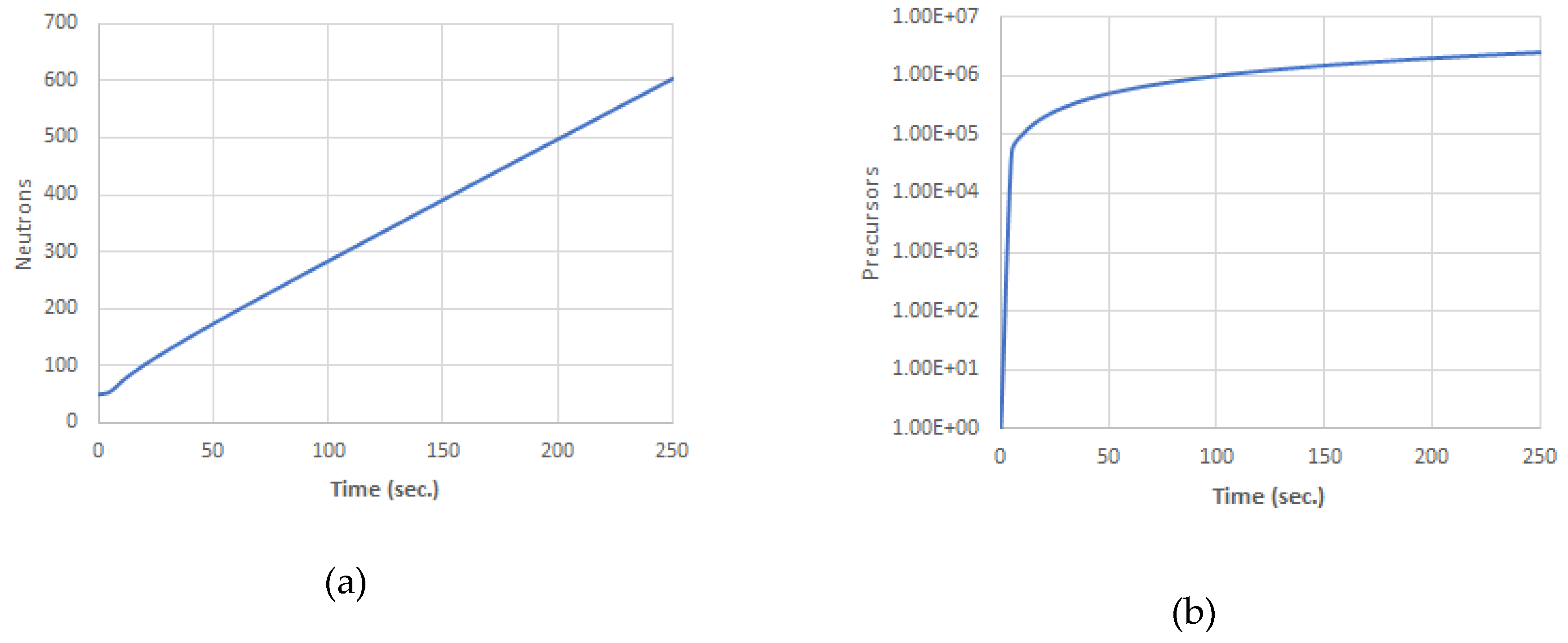
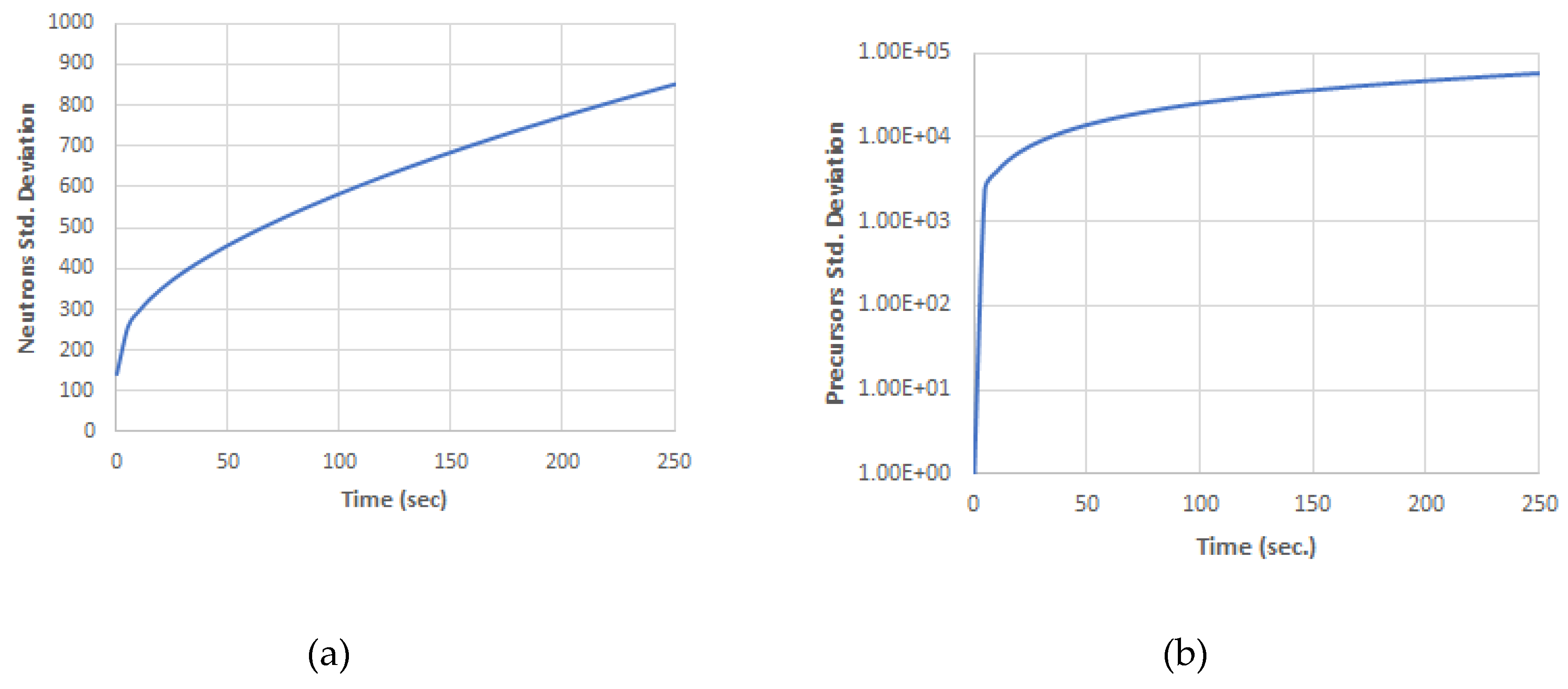
The results are shown in
Figure 1 and
Figure 2 and
Table 1 for different values of the parameter
. It is noted that the mean values of the neutronic power and the precursors are approximately the same for all values of,
as shown in
Figure 1. The standard variations of the neutronic power and the precursors increase proportionally with
, as in
Figure 2. The change in the neutronic power is relatively small (< 0.25% for
= 7.5%) and reaches a steady state rapidly. The change in the precursors are more sensitive (~ 4.0% for
= 7.5%) and propagate as the time increases.
Table 1 shows the variations of
and the corresponding standard deviations of the neutronic power
and the precursors
relative to mean values at time = 250 s. There is a linear relation between
and changes in both the power and the precursor density. The linear relation has a slope of only 3.1% for the power but it is 52.4% for the precursor density.
In the case whereby only noise variation is considered, the results are shown in
Figure 3 and
Table 2. The mean values are approximately the same as shown above in
Figure 1 and are not repeated here. The standard deviations for the neutronic power and the precursors increase rapidly with the time, as shown in
Figure 3. The standard deviations of the neutronic power is considerable and exceeds 140% of the mean values even if the external (or initial) source is neglected. For the precursors, the standard deviation is only around 2.5% of the mean value.
For further testing of the stochastic model, a second test case was considered and compared with [
19] and [
5]. The model had six precursor groups with step reactivity of 0.003,
(
s−1),
,
(
s),
,
,
(
s). The initial conditions were taken as
and
. The comparison shows consistency of the results with the literature work, as in
Table 2.
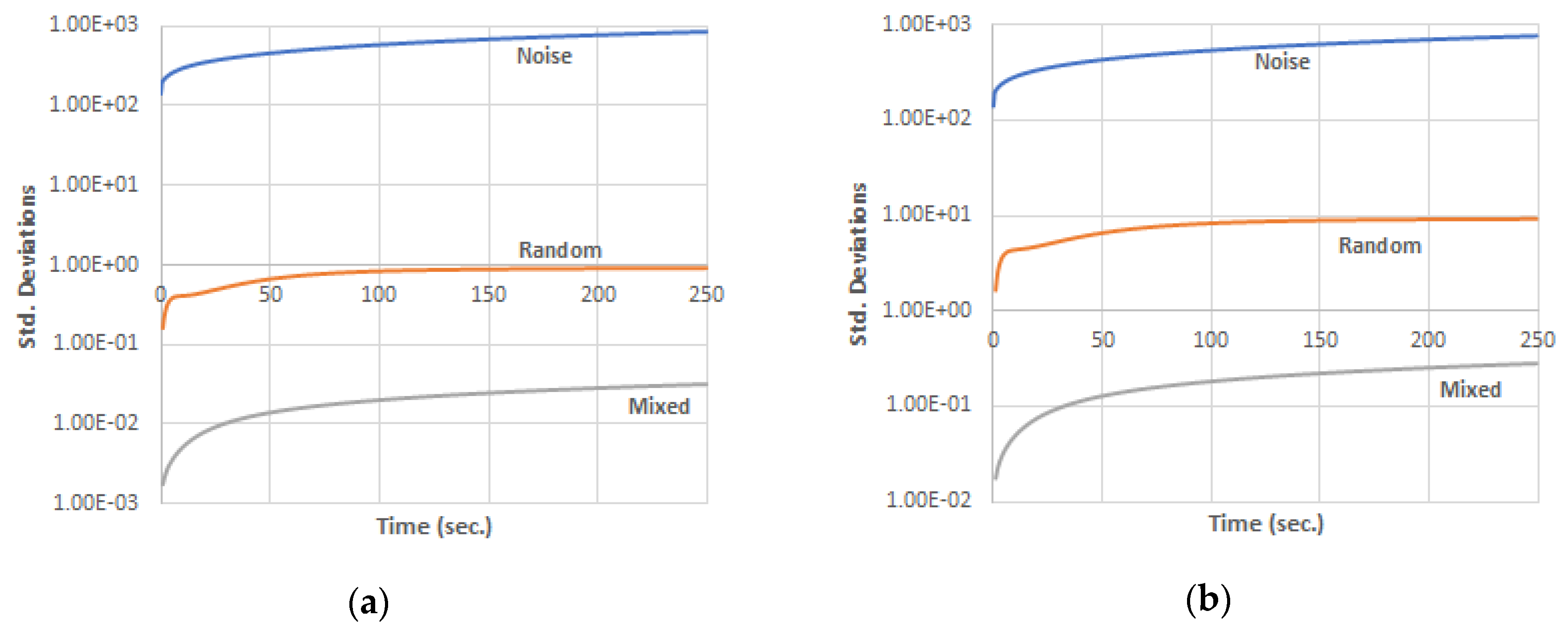
For the combined effect, both due to noise variations and random parameters, systems (13) and (14) are solved with the parameters in the first test case. For the random parameters, let
= 5.0% up to 100%.
Figure 4 shows the standard deviations due to noise, random, and mixed effects on the neutronic power in case of
= 5.0% and 50%.
Table 3 shows the deviations due to noise, random parameters, and the mixed effects for a wide range of
. Furthermore, the deviation due to noise is dominant. Additionally, both the random and mixed deviations proportionally increase with
. We can notice also that the mixed deviations are negligible compared with other deviations even for large values of
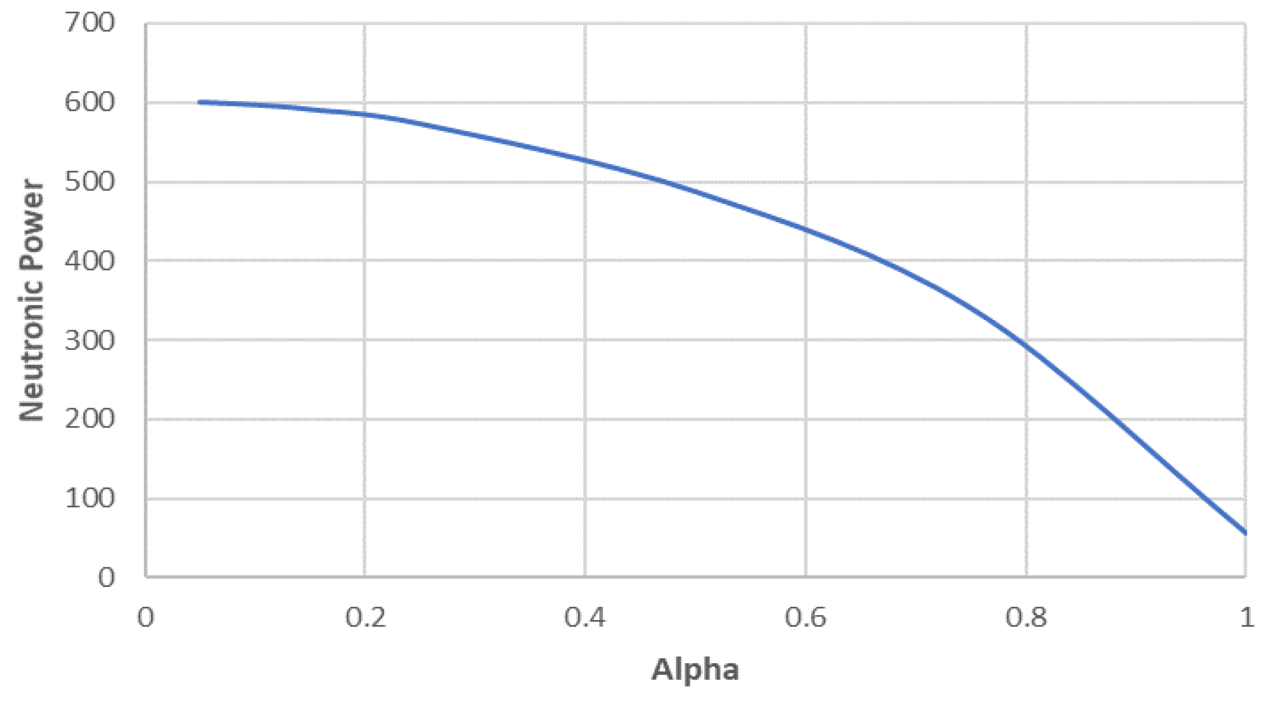
. The neutronic power decreases with the deviations due to the random parameters. Large deviations in the random parameters cause significant reduction in the neutronic power, as shown in
Figure 5.
The thermal hydraulics were estimated for the first case using the parameters shown in
Table 4. The inlet coolant temperature is
= 282 °C.
Figure 6 shows the deviations in the fuel temperature for
= 25%. We can notice that the temperature deviation reaches a steady state rapidly compared with the neutronic power and the precursor density. Deviations in the coolant temperature are obtained similarly.


