A Linear Regression Thermal Displacement Lathe Spindle Model

Abstract

Thermal error is one of the main reasons for the loss of accuracy in lathe machining. In this study, a thermal deformation compensation model is presented that can reduce the influence of spindle thermal error on machining accuracy. The method used involves the collection of temperature data from the front and rear spindle bearings by means of embedded sensors in the bearing housings. Room temperature data were also collected as well as the thermal elongation of the main shaft. The data were used in a linear regression model to establish a robust model with strong predictive capability. Three methods were used: (1) Comsol was used for finite element analysis and the results were compared with actual measured temperatures. (2) This method involved the adjustment of the parameters of the linear regression model using the indicators of the coefficient of determination, root mean square error, mean square error, and mean absolute error, to find the best parameters for a spindle thermal displacement model. (3) The third method used system recognition to determine similarity to actual data by dividing the model into rise time and stable time. The rise time was controlled to explore the accuracy of prediction of the model at different intervals. The experimental results show that the actual measured temperatures were very close to those obtained in the Comsol analysis. The traditional model calculates prediction error values within single intervals, and so the model was divided to give rise time and stable time. The experimental results showed two error intervals, 19µm in the rise time and 15µm in the stable time, and these findings allowed the machining accuracy to be enhanced.

1. Introduction

Modern machine tools, particularly those that process metal, have become very smart. High precision and accuracy in processing have become a very important requirement. Such machines used in production get hot, and thermal expansion is the main cause of errors in accuracy [1,2]. The source of the heat involved in thermal expansion can be internal, generated by the machine itself, or external from the environment [3]. The heat that causes thermal deformation of the main shaft, accounts for 40% to 70% [4] or 30% to 50% [5] of the thermal deformation in machine tools. There are several ways to reduce the effects of thermal expansion, and the most obvious is to compensate for the changes [6]. However, other approaches have been made which include: cooling the spindle to reduce expansion; maintaining the temperature of the spindle within a particular range to keep dimensional changes to a minimum; and conduction of the heat from a high temperature zone to another of the low temperature to keep the spindle temperature uniform and reduce irregular deformation. However, the establishment of a model to measure temperature, which can be used to determine thermal displacement of the spindle for which compensation is then made by means of a controller, is the easiest and most commonly used method [7]. Thermal error compensation involves: temperature and thermal deformation measurement, the establishment of an error model, and error compensation. To enhance machining accuracy, it is necessary to establish a stable and robust spindle thermal displacement prediction model [8,9]. Many studies have been made into the development of thermal error models. Tseng and Ho [10] proposed an accurate and fast method for measuring the differences between static thermal error and errors during actual cutting operations. They used the measured temperature and offset to establish models using multivariate linear regression and nonlinear exponential regression. The results showed that multiple linear regression and nonlinear exponential regression can limit the thermal error to within 5%. Furthermore, single variable nonlinear exponent regression can reduce the error by 40% to 60%. Cheng et al. [11] proposed a robust thermal displacement prediction model. By selecting the key temperature measurement points using grey relation theory, the number of points needed could be reduced from 24 to 7. The radial basis function (RBF) and back propagation neural network were then used to establish the model, the results showed that the prediction accuracy of the RBF neural network was better than the traditional back propagation neural network. Hou et al. [12] proposed a combination of a multi-objective genetic algorithm (MOGA) with an approximate physical model and spindle thermal performance test data to establish a thermal error prediction model. The results showed the model to be accurate and robust. Li and Li [13] proposed a gene expression programming algorithm (GEP) that enabled optimization of the penalty parameter and the kernel function parameter sigma in regression of the weighted least squares support vector machine (WLS-SVM). Their results showed that GEP-WLSSVM modeling was superior to the PSO-LSSVM and GA-LSSVM methods. Guo et al. [14] used grey relation theory to select five key temperature measurement points to optimize a back propagation neural network with the artificial fish swarm and ant colony algorithms. They used the artificial fish swarm to generate the initial value of the ant colony algorithm and improve the calculation speed and model prediction accuracy of the back propagation neural network. This reduced the thermal error after compensation from 23 µm to 10 µm. Tan et al. [15] used the minimum absolute contraction and selection operator to select the critical temperature point and reduced the number of original temperature measurement points from 20 to 7. They also established the support vector machine model using least squares and compared the results with the grey prediction and multiple linear regression models. The least squares support vector machines model enhanced prediction by 74.6% and 54.3%, respectively, compared with the color prediction and multiple linear regression models. This showed the SVM model to be valid and feasible. Xiang et al. [16] established a preliminary model theory of temperature field and thermal deformation through mechanism analysis of the spindle size and parameters of the bearings. They then carried out tests under two different initial temperature conditions, evaluated the test results and modified the preliminary theoretical model to obtain a final model. The amount of thermal deformation in the model was then simulated at different rotational speeds using finite element analysis. This showed the relationship between thermal deformation and velocity to be approximately linear, and prediction of the temperature field of the main shaft was accurate. Pahk and Lee. [17] used multiple linear regression, a neural network and system identification to establish thermal error models, and then evaluated and compared the models. Their results showed system identification to be the model with the least error and could be used to modify coordinates in a CNC controller and apply compensation that effectively enhanced accuracy. Fan et al. [18] proposed a thermal error model based on orthogonal polynomials; the polynomial regression was converted to more easily computed multiple linear regression using orthogonal polynomials, and the compensation method was based on external coordinate offset. The results showed a 90% error reduction. Tseng and Chen [19] used the neural-fuzzy theory to establish a thermal error prediction model and compared it with multi-variable linear regression analysis. The neural-fuzzy theory thermal error model enhanced the machining accuracy from 80 µm to 3 µm, while the multi-variable linear regression analysis enhanced the original machining accuracy to 10 µm. The results showed that the neural-fuzzy theory thermal error model was better than multi-variable linear regression analysis thermal error model and enhanced the machining accuracy from 10 µm to 3 µm. Jian et al. [20] used the general regression neural network to establish a thermal displacement model of the spindle; the results showed that the thermal prediction model established by using the general regression neural network was robust and had good prediction ability.

To reduce the influence of thermal error on machining accuracy, critical temperature measurement points and robust thermal error prediction models are required [21]. This article adopted a linear regression model to analyze the spindle thermal displacement of lathes. In this article, a laser displacement meter was used, which focused two infrared points on the object to be measured to obtain the displacement. However, the lathe can generate vibrations when running at high speed, affecting the foci of the infrared. In order to prevent the impact of vibrations on the model robustness and predictability, this article chose the linear regression model approach. At the same time, the optimum parameters of the model were adjusted to improve the robustness and prediction ability of the model, so the results could be close to the actual displacement. Newer modeling methods were not adopted for this study, as they might be affected by the vibrations, making the predicted results deviate from the actual values. [22]. This article selected a suitable model for the sensor and adopted three methods to increase the model robustness. The first method uses COMSOL to conduct finite element analysis and ensures the accuracy of temperature measurement. The second method adjusts the linear model parameters based on the spindle thermal displacement and finds the best parameters to improve the model robustness. The third method uses system identification to fit a system with highly similar actual data and define the rise time of the model. The model has risen time and stable time to explore the accuracy of prediction of model in different intervals. The three abovementioned methods were adopted to increase the model robustness.

2. Methods

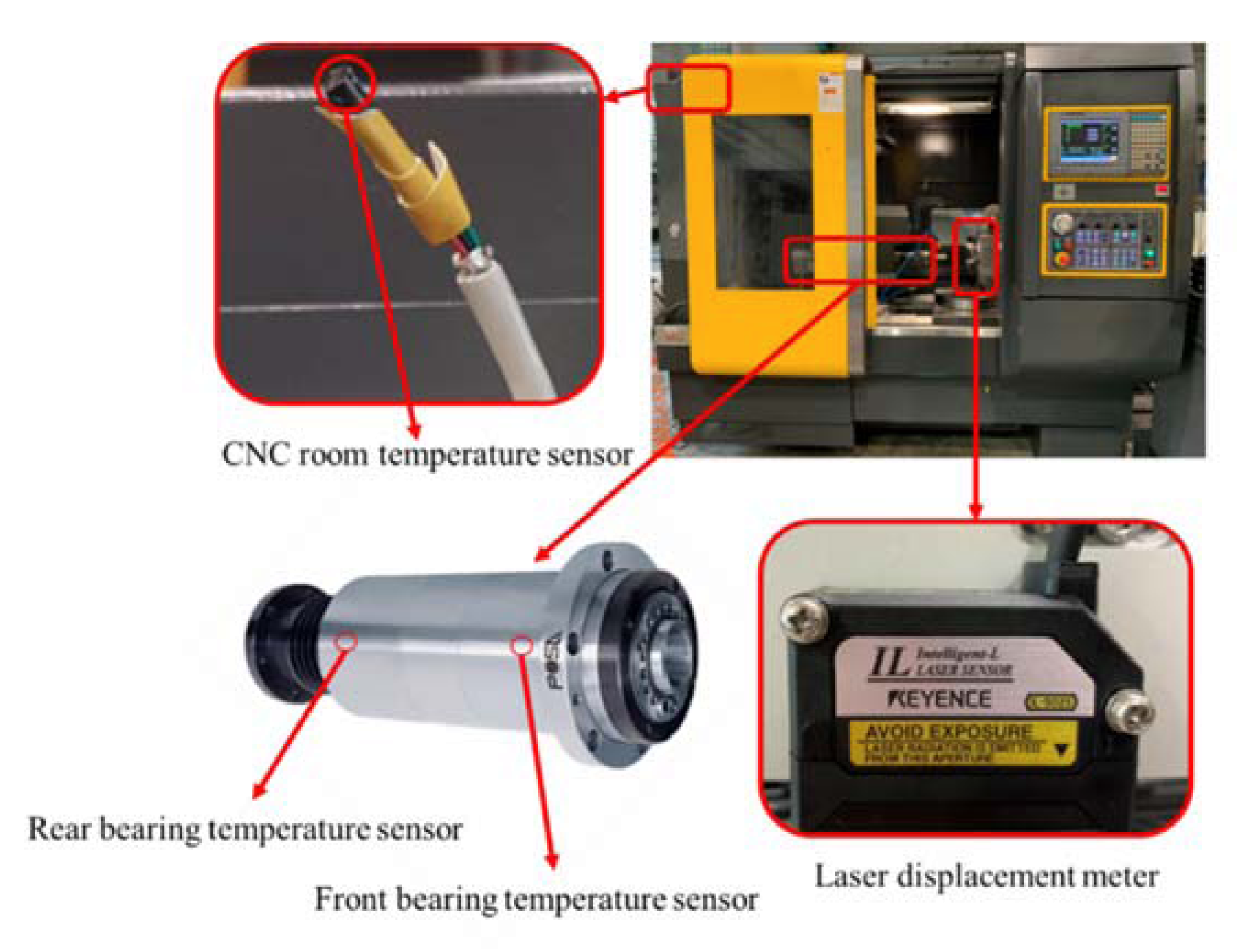
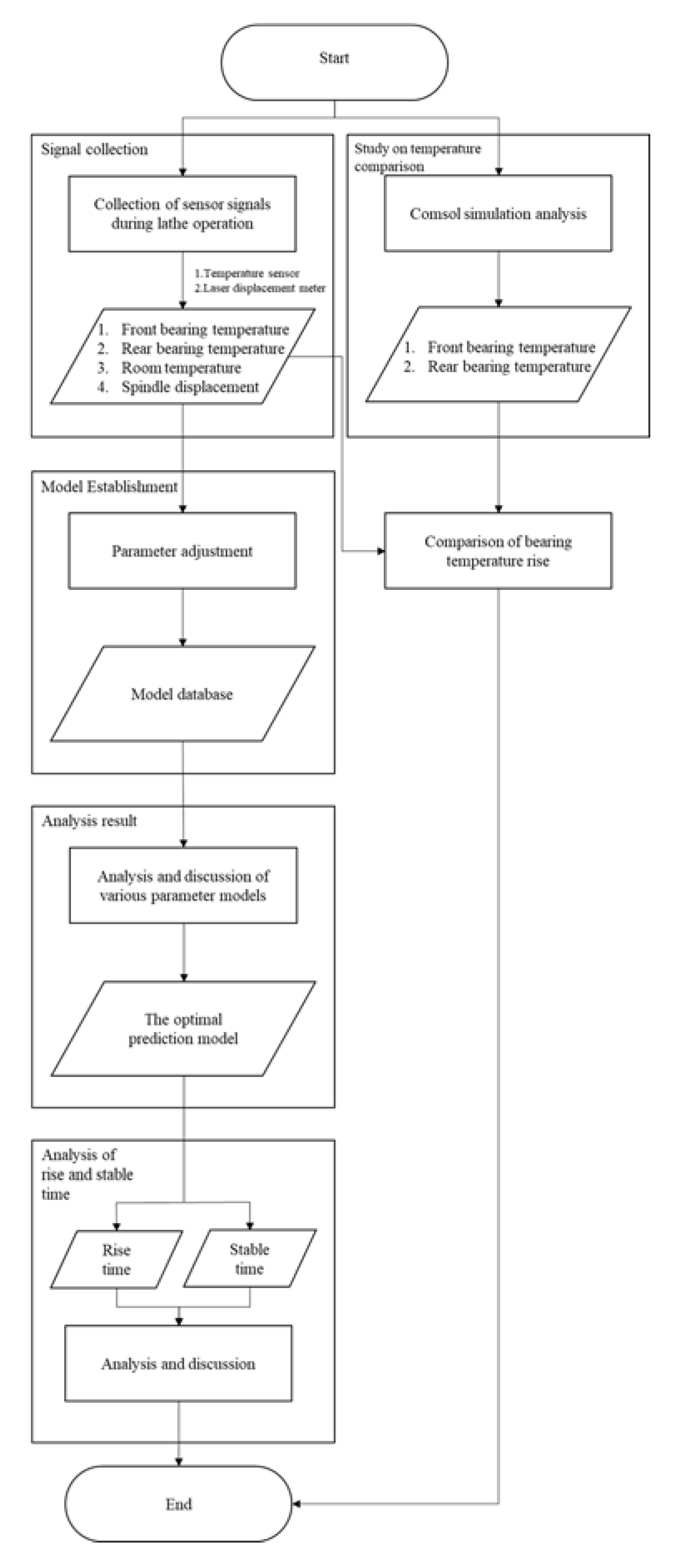
2.1. Experimental Equipment and Architecture

The machine tool used in these experiments was a Lathe (MC4200BL) with a POSA belt-driven spindle (TAC-10-CY) and a controller (SYNTEC21-TA). Contact digital temperature heat sensors (DS18B20), which have a measurement range of −55 °C to 125 °C and a resolution of 0.5 °C, were used to measure heat changes. The sampling frequency was 5 s. A temperature sensor was embedded in the front and rear main spindle bearings housing, as shown in Figure 1. Another sensor was used to measure the room temperature, see Figure 1. A laser displacement meter (IL-S025) was mounted on the lathe turret to measure the Z-axis offset of the spindle. The measurement range of this non-contact device was 20 mm to 30 mm with a resolution of 1 µm. Sampling frequency was 5 s. The positions of the measuring devices are shown in Figure 1. The experimental methods and procedures of this study are shown in Figure 2, divided into Comsol (version 5.2a) to implement finite element analysis, Comsol was used for analysis of the spindle temperature field, and the measurements of the actual temperature and offset of the machine tool turret. Accuracy of the actual measured data was verified by comparison of measured data with temperature analyzed by Comsol. The actual measured data were used to establish a linear regression model, and parameters were adjusted to enhance the robustness and prediction ability of the model. A search for the best prediction model was carried out using the actual measurement data to build the model. The coefficient of determination, root mean square error (RMSE), mean square error (MSE), and mean absolute error (MAE) were used, and the optimal parameter model found was used to control the rise time of the system.

2.1.1. Experimental Model

The Matlab 2018b linear regression learner toolbox was used to create the model. The model parameters were adjusted using linear regression as introduced in Section 2.1.2. The model specification parameters were introduced in Section 2.1.3 and the parameters of linear regression model (an indicator of the robust fitting type) in Section 2.1.4. To ensure the accuracy of the model, K-fold Cross-Validation (K-fold CV) of 20 was used, and the n-fold CV was used to divide the data into n sets at random, one was used as test data, the other for training and the process was repeated until each set had been used as test data [23,24]. Because a 20-fold CV was used, $n$ at the bottom was 20, see Figure 3. In the figure, $E_i$ is the error of the $i$th training, $E$ is the total error, and the total error of the model is the average of the error after 20 training sessions. The best parameter model was found by comparing the prediction ability of the coefficient of determination ($R^2$), root mean square error (RMSE), mean square error (MSE), and mean absolute error (MAE) as introduced in Section 2.3.

2.1.2. Linear Regression

Linear regression uses a linear line to fit the relationship between input and output. It can be used to explore the relationship between an independent and a dependent variable. The independent variable can also be used to predict the dependent variable. In this study, there were four inputs: from the front and rear spindle bearing temperature sensors, the room temperature sensor, and the laser displacement meter. The general linear regression equation is shown in (1), and the least square method was used to calculate the sum of the squared errors of all sample points, as shown in Equation (2) [25,26]:

$$Y={\beta }_0+{\beta }_1{x}_1+{\beta }_2{x}_2+{\beta }_3{x}_3+\epsilon$$

(1)

$$\epsilon ={\displaystyle \sum _{i=1}^{}(y_i-{\widehat{y}}_i}{)}^2$$

(2)

In the above equations, $x_{}$ is the independent variable, $Y$ is the dependent variable, ${\beta }_0$ is the constant term, ${\beta }_1$ is the coefficient of $x_1$, $\epsilon$ is the total error of the actual and predicted value, $y_i$ is the i th input value, and ${\widehat{y}}_i$ is the i th predicted value. The Linear Regression introduced in Section 2.1.1 is general linear-regression, and the linear-regression used in this study was introduced in Section 2.1.2.

2.1.3. Model Specification

Four types of model specification parameters were used in this study: the linear model, interactions model, pure quadratic model, and the quadratic model. In the linear model, linear prediction functions were used to model the relationships. The unknown model parameters of the functions were estimated from the data. To solve the sparsity problem, the interactions model used the idea of matrix decomposition; a large sparse matrix was decomposed into two hidden matrices. The dimensions of the hidden matrices are usually much smaller than that of the original matrix, so the sparsity problem can be effectively reduced. Quadratic regression can find an equation for a parabola that best fits a set of data. The pure quadratic regression model has square terms for each attribute. In linear regression, the prediction of a dependent attribute is a clone using single independent attributes and is not collective [27]. The equations of the different parameter models are shown in

Table 1. Extension element model showing when islanding will occur.

Model	Equations
Linear	$\mathrm{Y}={\beta }_0+{\beta }_1\times x_1+{\beta }_2\times x_2+{\beta }_3\times x_3$
Interactions	$\begin{array}{ll}\mathrm{Y}& ={\beta }_0+{\beta }_1\times x_1\times x_2\\ & +{\beta }_2\times x_1\times x_3+{\beta }_3\times x_2\times x_3\end{array}$
Pure quadratic	$\begin{array}{ll}\mathrm{Y}& ={\beta }_0+{\beta }_1\times x_1+{\beta }_2\times x_2+{\beta }_3\times x_3\\ & +{\beta }_4\times x_1^2+{\beta }_5\times x_2^2+{\beta }_6\times x_3^2\end{array}$
Quadratic	$\begin{array}{ll}\mathrm{Y}& ={\beta }_0+{\beta }_1\times x_1\times x_2+{\beta }_2\times x_1\times x_3\\ & +{\beta }_3\times x_2\times x_3+{\beta }_4\times x_1^2\\ & +{\beta }_5\times x_2^2+{\beta }_6\times x_3^2\end{array}$

Note: ${\beta }_0$ is the constant term, ${\beta }_i$ is the $i^{th}$ coefficient.

.

2.1.4. Indicator of the Robust Fitting Type

The robust weight function was mainly used to adjust the weight. The disadvantage of the least squares method in linear regression is its sensitivity to outliers, which have a substantial influence on fit. To improve the influence of the extremum on model fitting, nine types of robust weight function were used in this study to adjust the weight. The purpose of adjusting the weight was to increase the value of points near the fitted line and to reduce the value of the extremum or outliers; this reduces the influence of extremum on fitting. A robust fit will follow the bulk of the data and reduce the impact of outliers or extremum on the model, see equations in

Table 2. Robust Weight Functions.

Robust Weight Function	Equation	Default Tuning Constant
Andrews	$w=\frac{(\mathrm{abs}(r)<pi)\times \sin (r)}{r}$	1.339
Bisquare	$w=(\mathrm{abs}(r)<1)\times {(1-r^2)}^2$	4.685
Cauchy	$w=\frac{1}{(1+r^2)}$	2.385
Fair	$w=\frac{1}{(1+\mathrm{abs}(r))}$	1.4
Huber	$w=\frac{1}{\max (1,\mathrm{abs}(r))}$	1.345
Logistic	$w=\frac{\tanh (r)}{r}$	1.205
Ordinary least squares	Ordinary least squares (no weighting function)	None
Talwar	$w=1\times (\mathrm{abs}(r)<1)$	2.795
Welsch	$w={\mathrm{e}}^{(-r^2)}$	2.985

[28,29,30].

$r$ is shown as (3)

$$r=\frac{resid}{(tune\times s\times \mathrm{sqrt}(1-h))}$$

(3)

where $resid$ is the vector of residuals from the previous iteration, $h$ is the vector of leverage values from a least-squares fit, $tune$ is a tuning constant that is divided into the residual vector before computing weights, and $s$ is an estimate of the standard deviation of the error term:

$$s=\frac{MAD}{0.6745}$$

(4)

$MAD$ is the median absolute deviation of the residuals from their median. The constant 0.6745 makes the estimate unbiased for normal distribution.

2.2. Calculation of the Relationship between Speed and Temperature Rise

Friction in the bearings generates heat, and this is reflected as a rise in temperature measured by the sensors embedded in the bearing housing. The resulting heat-deformation of the spindle is also reflected by the temperature field presented by Comsol analysis of the spindle. The displacement that results from this rise in temperature is measured by the laser displacement meter. The higher the speed of rotation, the higher the temperature and the greater the deformation. The calculation equation of the bearing heat is shown in (5); the ball bearing equation is calorific and the value can be expressed as (6) [20,31,32]:

$$Q=1.047\times {10}^{-4}\times n\times M$$

(5)

$$Q=0.0525\times \mu \times d\times F\times n$$

(6)

In the above equations, $Q$ is the heat generated (W); $n$ is the rotational speed (rpm); $d$ is inner diameter of the bearing (m); and $F$ is the load of the bearing (N). It can be seen from (5) that when other conditions remain unchanged, rotation speed $n$ is proportional to calorific value $Q$. The higher the rotation speed, the higher the heat.

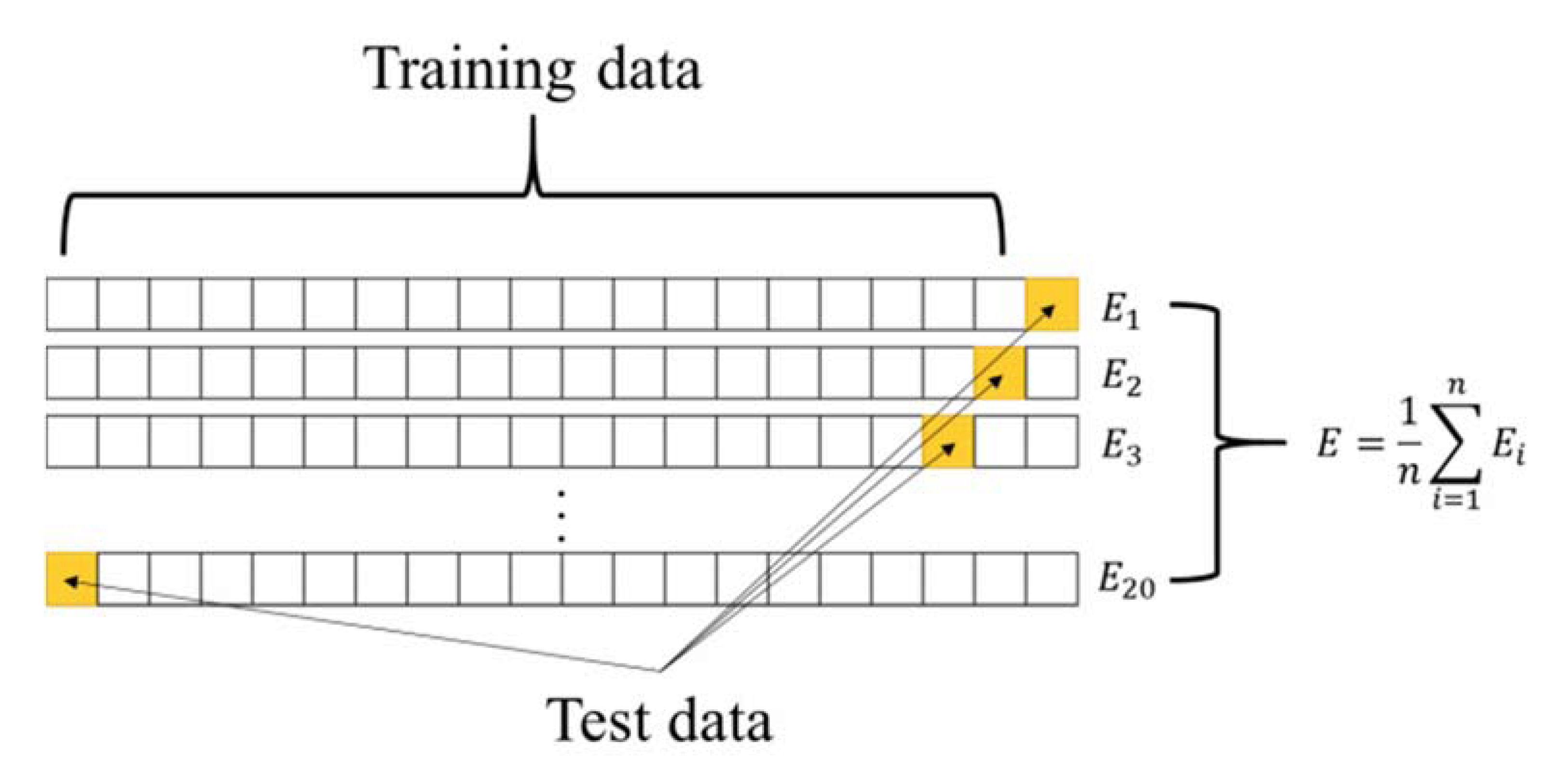
2.3. Model Verification Coefficient

The coefficient of determination ($R^2$), root mean square error (RMSE), mean square error (MSE), and mean absolute error (MAE) were used to verify the prediction ability of each parameter model.

The coefficient of determination has a value between $0<R^2<1$, the closer the value to 1, the better the prediction ability of the model, the equation is shown as (7) [33]:

$$R^2=1-\frac{S{S}_{res}}{S{S}_{tot}}$$

(7)

In Equation (7), SS_res is the residual sum of the squares, and SS_tot is the total sum of the squares.

RMSE, MSE and MAE are used to calculate the error of the actual and prediction values; the smaller the error, the better the prediction of the model; the followings three Equations (8)–(10) can be used to calculate the error [34]:

$$RMSE=\sqrt{\frac{1}{n}{\displaystyle \sum _{i=1}^n{({\widehat{y}}_i-y_i)}^2}}$$

(8)

$$MSE=\frac{1}{n}{\displaystyle \sum _{i=1}^n{({\widehat{y}}_i-y_i)}^2}$$

(9)

$$MAE=\frac{1}{n}{\displaystyle \sum _{i=1}^n|{\widehat{y}}_i-y_i|}$$

(10)

In the above equations, ${\widehat{y}}_i$ is the $i$th prediction value, and $y_i$ is the $i$th actual value.

3. Results and Discussions

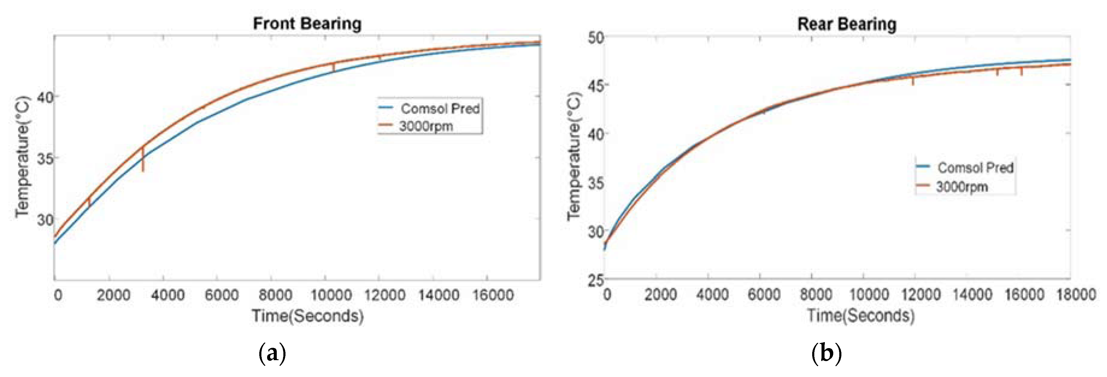
3.1. Comsol Analysis

In this study, the 3D structural model of the spindle was loaded into the finite element analysis program Comsol, and the material properties were set as S45C, SCM440, SCM415, and FC20. The heat source load was calculated according to Section 2.3, and the generated starting heat volume was 18.92 W [20]. The temperature rise calculated by the Comsol program for the front and rear bearings of the machine spindle were plotted against time and compared with actual measured temperatures obtained from an operating machine. Figure 4 shows the results obtained for the front and rear bearing.

In this study, the thermal convection boundary condition was air; in a normal working environment, the free convection is about 10 to 20 (w/m2k) and the forced convection is 50 to 250 (w/m2k). In a belt-driven spindle, the motor drives the spindle axis and collet rotation to have forced convection. The COMSOL in this study simulated a natural convection at 15 (w/m2k) and a forced convection at 100 (w/m2k), and the grid area of the spindle axis in this study was larger. As the heat source of the spindle axis is at the bearing, it is necessary to discuss the bearing temperature. This study set the grids near the bearing thinner. The total number of nodes were 2819 and the grid element was 5582. Figure 5 shows the schematic picture of the model.

The plots in Figure 4 show that the maximum errors in the Comsol finite analysis of the temperatures of the front and rear bearings are within 1 °C [20] of the actual measured value, indicating that the measured data is highly accurate.

3.2. Linear Regression Model Establishment and Parameter Adjustment

Linear regression was used to establish the model and adjust the model specification and indicator robust fitting parameters. In addition, a K-fold CV value of 20 was used with the coefficient of determination, root mean square error (RMSE), mean square error (MSE), and mean absolute rrror (MAE) to verify the prediction ability of each model.

To find the optimal parameter model, combinations of four different model specification parameters and nine robust weight function parameters were used. The coefficient of determination ($R^2$) for each parameter model is shown in

Table 3. The $R^2$ of the combination of four kinds of model specification parameters and nine kinds of robust weight function parameters.

${\mathit{R}}^2$	Linear Model	Interactions Model	Pure Quadratic Model	Quadratic Model
Andrews	0.976447776	0.985206658	0.986315629	0.987897428
Bisquare	0.976446436	0.985210897	0.986321702	0.987890926
Cauchy	0.976446063	0.985446282	0.986379913	0.987893853
Fair	0.976453158	0.985544495	0.986415054	0.987896656
Huber	0.976445855	0.985434324	0.986359045	0.987890844
Logistic	0.976443716	0.985497259	0.986394534	0.987896652
Ordinary least squares	0.976489603	0.98565211	0.98647194	0.987913665
Talwar	0.976480432	0.985129585	0.98618952	0.987909337
Welsch	0.976438028	0.985338684	0.986344533	0.987895726

, the root mean square error (RMSE) is shown in

Table 4. The RMSE of the combination models of four kinds of model specification parameters and nine kinds of robust weight function parameters.

$\mathit{R}\mathit{M}\mathit{S}\mathit{E}$	Linear Model	Interactions Model	Pure Quadratic Model	Quadratic Model
Andrews	0.000802692	0.00063616	0.000611851	0.000575403
Bisquare	0.000802715	0.000636069	0.000611715	0.000575557
Cauchy	0.000802722	0.000630987	0.000610412	0.000575488
Fair	0.000802601	0.000628854	0.000609624	0.000575421
Huber	0.000802725	0.000631246	0.00061088	0.000575559
Logistic	0.000802762	0.000629881	0.000610084	0.000575421
Ordinary least squares	0.000801979	0.000626509	0.000608346	0.000575017
Talwar	0.000802136	0.000637815	0.000614664	0.00057512
Welsch	0.000802858	0.000633315	0.000611204	0.000575443

, mean square error (MSE) in

Table 5. The MSE of combination models of four kinds of model specification parameters and nine kinds of robust weight functions.

$\mathit{M}\mathit{S}\mathit{E}$	Linear Model	Interactions Model	Pure Quadratic Model	Quadratic Model
Andrews	6.44315 $\times {10}^{-7}$	4.047 $\times {10}^{-7}$	3.74362 $\times {10}^{-7}$	3.31088 $\times {10}^{-7}$
Bisquare	6.44352 $\times {10}^{-7}$	4.04584 $\times {10}^{-7}$	3.74195 $\times {10}^{-7}$	3.31266 $\times {10}^{-7}$
Cauchy	6.44362 $\times {10}^{-7}$	3.98144 $\times {10}^{-7}$	3.72603 $\times {10}^{-7}$	3.31186 $\times {10}^{-7}$
Fair	6.44168 $\times {10}^{-7}$	3.95457 $\times {10}^{-7}$	3.71642 $\times {10}^{-7}$	3.3111 $\times {10}^{-7}$
Huber	6.44368 $\times {10}^{-7}$	3.98471 $\times {10}^{-7}$	3.73174 $\times {10}^{-7}$	3.31269 $\times {10}^{-7}$
Logistic	6.44426 $\times {10}^{-7}$	3.9675 $\times {10}^{-7}$	3.72203 $\times {10}^{-7}$	3.3111 $\times {10}^{-7}$
Ordinary least squares	6.43171 $\times {10}^{-7}$	3.92513 $\times {10}^{-7}$	3.70085 $\times {10}^{-7}$	3.30644 $\times {10}^{-7}$
Talwar	6.43422 $\times {10}^{-7}$	4.06808 $\times {10}^{-7}$	3.77811 $\times {10}^{-7}$	3.30763 $\times {10}^{-7}$
Welsch	6.44582 $\times {10}^{-7}$	4.01088 $\times {10}^{-7}$	3.73571 $\times {10}^{-7}$	3.31135 $\times {10}^{-7}$

, and mean absolute error (MAE) in

Table 6. The MAE combination models of four kinds of model specification parameters, and nine kinds of robust weight function parameters.

$\mathit{M}\mathit{A}\mathit{E}$	Linear Model	Interactions Model	Pure Quadratic Model	Quadratic Model
Andrews	0.000637552	0.000490825	0.000481137	0.00046259
Bisquare	0.000637602	0.000490923	0.000481097	0.000462721
Cauchy	0.000637494	0.000491214	0.000481243	0.000462623
Fair	0.000637465	0.000491784	0.000481569	0.000462626
Huber	0.000637544	0.000491124	0.000481322	0.000462661
Logistic	0.000637485	0.000491222	0.000481383	0.000462658
Ordinary least squares	0.000639	0.00049515	0.000483696	0.000463451
Talwar	0.000638257	0.000491219	0.000481589	0.000463127
Welsch	0.000637655	0.000490858	0.000481141	0.00046266

.

The $R^2$ value lies between 0 and 1, and the closer it is to 1, the higher the prediction ability. The results in Table 3 show that the best parameter model specification is quadratic. The robust weight function was established by ordinary least squares, where $R^2$ is 0.987913, both are higher than the models established by other parameters combinations. For $R^2$, the best parameter model specification is quadratic, and the robust weight function of the ordinary least squares model has the best prediction ability.

RMSE is the root mean square error, the smaller it is the better the prediction value and the closer it is to the actual value. The results in Table 3 show that the best parameter model specification is quadratic. The robust weight function was established by ordinary least squares. The RMSE is 0.000575017, which is lower than the models established by other parameter combinations. For RMSE, the prediction values of the parameter model specification are quadratic, and the robust weight function for the ordinary least squares model is the closest to the actual value.

MSE is the mean square error, the smaller the error the better the prediction value and the closer it is to the actual value. The results in Table 5 show that the best parameter model specification is quadratic, and the robust weight function was established by ordinary least squares. Its MSE was 3.30644 $\times {10}^{-7}$, which is lower than in the models established by a combination of other parameters. For MSE, the prediction value of the parameter model specification is quadratic, and the robust weight function of the ordinary least squares model is closest to the actual value.

MAE is the mean absolute error, the smaller it is, the closer the prediction value of the model is to the actual value. The results in Table 6 show that the parameter model specification is quadratic, and the robust weight function is the model established by Andrews. Its MAE is 0.00046259, which is lower than in models established by other parameter combinations. For $MSE$, the prediction value of the parameter model specification is quadratic, and the robust weight function for the Andrews ordinary least squares model is closest to the actual value.

The results from Table 3 to Table 6 show that the adjustment parameter robust weight function has little impact on the prediction ability of the model. From the adjustment parameter model specification, it can be seen that the linear model only contains the intercept and linear terms of each predictor variable, and it cannot completely predict the spindle thermal deformation possible in the other models. The quadratic model, which includes an intercept, linear terms, interactions, and squared terms, can completely predict the spindle thermal deformation unlike the other models. In addition, $R^2$, $RMSE$, and $MSE$ indicate that the quadratic model and robust weight function for ordinary least squares have the best prediction ability compared to the others. Therefore, the quadratic model and robust weight function for ordinary least squares was selected as the best model. The displacement fit figure of the best parameter model is shown in Figure 6.

An examination of Figure 6 shows that before 8000 s, the displacement prediction value is close to the actual value, but after 8000 s, there is a significant difference between the displacement prediction value and the actual value. Therefore, in this study, model rise time and stable time have been separated according to the control system for further discussion.

3.3. Discussion on the Rise Time and Stable Time of the Optimal Parameter Model

In this study, rise time and stable time in the best parameter model are discussed separately. This discrimination is based on Matlab 2018b System Identification Toolbox 9.9, the Number of poles used was two, the Number of zeros was zero, and the Generalized Poisson Moment Functions approach was used for initialization [35] to find the transfer function of the model, as shown in (11). Rise time and stable time were separated by the control system, and rise time was 10% to 90% of the final value. When stable time was 90% of the final value, the rise time and stable time of the model were as shown in Figure 7; the thermal displacement fit Figure for the rise time and stable time of the optimal parameter is shown in Figure 8.

$$G(s)=\frac{7.185\times {10}^{-10}}{s^2+ 0.0004507s+2.938\times {10}^{-8}}$$

(11)

Figure 8 shows that the prediction model has two parts: rise time and stable time, with different error intervals, 19 µm and 15 µm. Adjustment of the prediction error values at different times can reveal the prediction ability of the model more accurately and enhance the robustness and effectiveness of the model.

4. Conclusions

To reduce the influence of spindle thermal error on machining accuracy, a robust and effective thermal error model was established that could be used to predict the spindle thermal elongation and compensate for this using a controller. The quality of the model had a direct effect on accuracy. The main contribution of the article is in selecting a suitable model for the sensor and adopting three methods to increase the model robustness. The first method is using COMSOL to conduct finite element analysis and ensures the accuracy of temperature measurement. The second method adjusts the linear model parameters based on the spindle thermal displacement and finds the best parameters to improve the model robustness. The third method uses system identification to fit a system with highly similar actual data and defines the rise time of the model. The model has risen time and stable time to explore the accuracy of prediction of the model in different intervals. The abovementioned three methods were adopted to increase the model robustness. The actual displacement error value and the predicted displacement value of the model rise time were within 19 µm of the actual displacement value and that of the stable time was within 15 µm.

References

1. Li, Y.; Zhao, W.H.; Lan, S.H.; Ni, J.; Wu, W.W.; Lu, B.H. A review on spindle thermal error compensation in machine tools. Int. J. Mach. Tools Manuf. 2015, 95, 20–38. [Google Scholar] [CrossRef]
2. Huang, J.; Zhou, Z.D.; Liu, M.Y.; Zhang, E.L.; Chen, M.; Pham, D.T.; Ji, C.Q. Real-time measurement of temperature field in heavy-duty machine tools using fiber Bragg grating sensors and analysis of thermal shift errors. Mechatronics 2015, 31, 16–21. [Google Scholar] [CrossRef]
3. Abdulshahed, A.M.; Longstaff, A.P.; Fletcher, S. The application of ANFIS prediction models for thermal error compensation on CNC machine tools. Appl. Soft Comput. 2015, 27, 158–168. [Google Scholar] [CrossRef]
4. Bryan, J. International Status of Thermal Error Research. CIRP Ann. 1990, 39, 645–656. [Google Scholar] [CrossRef]
5. Liu, K.; Liu, Y.; Sun, M.J.; Li, X.L.; Wu, Y.L. Spindle axial thermal growth modeling and compensation on CNC turning machines. Int. J. Adv. Manuf. Technol. 2016, 87, 2285–2292. [Google Scholar] [CrossRef]
6. Du, Z.C.; Yao, S.Y.; Yang, J.G. Thermal Behavior Analysis and Thermal Error Compensation for Motorized Spindle of Machine Tools. Int. J. Precis. Eng. Manuf. 2015, 16, 1571–1581. [Google Scholar] [CrossRef]
7. Chen, T.C.; Chang, C.J.; Hung, J.P.; Lee, R.M.; Wang, C.C. Real-Time Compensation for Thermal Errors of the Milling Machine. Appl. Sci. 2016, 6, 101. [Google Scholar] [CrossRef] [Green Version]
8. Zhang, T.; Ye, W.H.; Shan, Y.C. Application of sliced inverse regression with fuzzy clustering for thermal error modeling of CNC machine tool. Int. J. Adv. Manuf. Technol. 2016, 85, 9–12. [Google Scholar] [CrossRef]
9. Li, Y.; Zhao, J.; Ji, S.J.; Liang, F.S. The selection of temperature-sensitivity points based on K-harmonic means clustering and thermal positioning error modeling of machine tools. Int. J. Adv. Manuf. Technol. 2019, 100, 2333–2348. [Google Scholar] [CrossRef]
10. Tseng, P.C.; Ho, J.L. A study of high-precision CNC lathe thermal errors and compensation. Int. J. Adv. Manuf. Technol. 2002, 19, 850–858. [Google Scholar] [CrossRef]
11. Cheng, Q.; Qi, Z.; Zhang, G.J.; Zhao, Y.S.; Sun, B.W.; Gu, P.H. Robust modelling and prediction of thermally induced positional error based on grey rough set theory and neural networks. Int. J. Adv. Manuf. Technol. 2016, 83, 753–764. [Google Scholar] [CrossRef]
12. Hou, R.S.; Du, H.Y.; Yan, Z.Z.; Yu, W.B.; Tao, T.; Mei, X.S. The modeling method on thermal expansion of CNC lathe headstock in vertical direction based on MOGA. Int. J. Adv. Manuf. Technol. 2019, 103, 3629–3641. [Google Scholar] [CrossRef]
13. Li, Q.; Li, H.L. A general method for thermal error measurement and modeling in CNC machine tools’ spindle. Int. J. Adv. Manuf. Technol. 2019, 103, 2739–2749. [Google Scholar] [CrossRef]
14. Guo, Q.J.; Xu, R.F.; Yang, T.Y.; He, L.; Cheng, X.; Li, Z.Y.; Yang, J.G. Application of GRAM and AFSACA-BPN to thermal error optimization modeling of CNC machine tools. Int. J. Adv. Manuf. Technol. 2016, 83, 995–1002. [Google Scholar] [CrossRef]
15. Tan, F.; Yin, M.; Wang, L.; Yin, G.F. Spindle thermal error robust modeling using LASSO and LS-SVM. Int. J. Adv. Manuf. Technol. 2018, 94, 2861–2874. [Google Scholar] [CrossRef]
16. Xiang, S.T.; Zhu, X.L.; Yang, J.G. Modeling for spindle thermal error in machine tools based on mechanism analysis and thermal basic characteristics tests. Proc. Inst. Mech. Eng. Part C J. Mech. Eng. Sci. 2014, 228, 3381–3394. [Google Scholar] [CrossRef]
17. Pahk, H.J.; Lee, S.W. Thermal error measurement and real time compensation system for the CNC machine tools incorporating the spindle thermal error and the feed axis thermal error. Int. J. Adv. Manuf. Technol. 2002, 20, 487–494. [Google Scholar] [CrossRef]
18. Fan, K.G.; Yang, J.G.; Yang, L.Y. Orthogonal polynomials-based thermally induced spindle and geometric error modeling and compensation. Int. J. Adv. Manuf. Technol. 2013, 65, 9–12. [Google Scholar] [CrossRef]
19. Tseng, P.C.; Chen, S.L. The neural-fuzzy thermal error compensation controller on CNC machining center. JSME Int. J. Ser. C Mech. Syst. Mach. Elem. Manuf. 2002, 45, 470–478. [Google Scholar] [CrossRef] [Green Version]
20. Jian, B.-L.; Wang, C.-C.; Hsieh, C.-T.; Kuo, Y.-P.; Houng, M.-C.; Yau, H.-T. Predicting spindle displacement caused by heat using the general regression neural network. Int. J. Adv. Manuf. Technol. 2019, 104, 4665–4674. [Google Scholar] [CrossRef]
21. Wei, X.; Gao, F.; Li, Y.; Zhang, D.Y. Study on optimal independent variables for the thermal error model of CNC machine tools. Int. J. Adv. Manuf. Technol. 2018, 98, 664–669. [Google Scholar] [CrossRef]
22. Shen, H.Y.; Sun, L.; Zhang, L.C.; Sha, J.F.; Liu, X.H.; Fu, J.Z. Position-independent thermal error compensation and evaluation based on linear correlation filtering technology. Int. J. Adv. Manuf. Technol. 2018, 95, 1357–1367. [Google Scholar]
23. Fushiki, T. Estimation of prediction error by using K-fold cross-validation. Stat. Comput. 2011, 21, 137–146. [Google Scholar] [CrossRef]
24. Wong, T.T.; Yang, N.Y. Dependency Analysis of Accuracy Estimates in k-Fold Cross Validation. IEEE Trans. Knowl. Data Eng. 2017, 29, 2417–2427. [Google Scholar] [CrossRef]
25. Fávero, L.P.; Belfiore, P. Simple and Multiple Regression Models. In Data Science for Business and Decision Making; Fávero, L.P., Belfiore, P., Eds.; Academic Press: Cambridge, MA, USA, 2019; pp. 443–538. [Google Scholar]
26. Li, Y.; Zhao, J.; Ji, S.J. A reconstructed variable regression method for thermal error modeling of machine tools. Int. J. Adv. Manuf. Technol. 2017, 90, 3673–3684. [Google Scholar] [CrossRef]
27. Shastry, A.; Sanjay, H.; Bhanusree, E. Prediction of Crop Yield Using Regression Techniques. Int. J. Soft Comput. 2017, 12, 96–102. [Google Scholar]
28. Andrews, D.F. A Robust Method for Multiple Linear Regression. Technometrics 1974, 16, 523–531. [Google Scholar] [CrossRef]
29. Polat, E. The effects of different weight functions on partial robust M-regression performance: A simulation study. Commun. Stat.-Simul. Comput. 2019, 1–16. [Google Scholar] [CrossRef]
30. Holland, P.W.; Welsch, R.E. Robust regression using iteratively reweighted least-squares. Commun. Stat.-Theory Methods 2007, 6, 813–827. [Google Scholar] [CrossRef]
31. Liu, K.; Sun, M.J.; Wu, Y.L.; Zhu, T.J. Thermal Error Modeling Method for a CNC Machine Tool Feed Drive System. Math. Prob. Eng. 2015, 4, 1–6. [Google Scholar] [CrossRef] [Green Version]
32. Feng, W.L.; Li, Z.H.; Gu, Q.Y.; Yang, J.G. Thermally induced positioning error modelling and compensation based on thermal characteristic analysis. Int. J. Mach. Tools Manuf. 2015, 93, 26–36. [Google Scholar] [CrossRef]
33. Dai, Y.; Guo, J.; Yang, L.; You, W. A New Approach of Intelligent Physical Health Evaluation based on GRNN and BPNN by Using a Wearable Smart Bracelet System. Proc. Comput. Sci. 2019, 147, 519–527. [Google Scholar] [CrossRef]
34. Yang, H.; Li, X.; Wu, B. Scale Forecast Method for Regional Highway Network Based on BPNN-MOP. Trans. Res. Proc. 2017, 25, 3840–3854. [Google Scholar] [CrossRef]
35. Garnier, H.; Mensler, M.; Richard, A. Continuous-time model identification from sampled data: Implementation issues and performance evaluation. Int. J. Control 2003, 76, 1337–1357. [Google Scholar] [CrossRef]
Figure 1. Position of the front and rear bearing temperature sensors, the room temperature sensor and the laser displacement meter.
Energies 13 00949 g001
Figure 2. Study flow chart.
Energies 13 00949 g002
Figure 3. n-fold Cross-Validation.
Energies 13 00949 g003
Figure 4. (a) Plot of front-bearing temperature rise from a Comsol analysis compared to actual measurements. (b) Plot of rear-bearing temperature rise from a Comsol analysis compared to actual measurements [20].
Energies 13 00949 g004
Figure 5. Schematic picture of the Model.
Energies 13 00949 g005
Figure 6. Displacement fit plot of the model predicted displacement value and actual value using the best model parameters.
Energies 13 00949 g006
Figure 7. (a) The rise time, which is 10% to 90% of the final value. Ten percent to 90% was used as the final rise time value of the model, and the other 90% was stable time. (b) The fit diagram of the system identification and actual displacement; the two-order system fits the actual displacement value very well.
Energies 13 00949 g007
Figure 8. Fit Diagram of the rise time and stable time of the optimal parameter spindle thermal displacement model. In (a), the difference of actual displacement value and predicted displacement value is within 19 µm. In (b), the difference between actual displacement value and predicted displacement value is within 15 µm.
Energies 13 00949 g008