Article

Direct Voltage Control of a Doubly Fed Induction Generator by Means of Optimal Strategy

by
Arthur Medeiros
1,*,
Thales Ramos
2,
José Tavares de Oliveira
3 and
Manoel F. Medeiros Júnior
4
1
Federal Institute of Education, Science and Technology of Rio Grande do Norte, Campus Natal – Zona Norte, Natal 59112-490, Brazil
2
Federal Institute of Education, Science and Technology of Rio Grande do Norte, Campus Santa Cruz, Santa Cruz 59200-000, Brazil
3
Department of Electrical Engineering, Federal University of Rio Grande do Norte, Natal 59078-970, Brazil
4
Department of Computer Engineering and Automation, Federal University of Rio Grande do Norte, Natal 59078-970, Brazil
*
Author to whom correspondence should be addressed.
Energies 2020, 13(3), 770; https://doi.org/10.3390/en13030770
Submission received: 4 December 2019 / Revised: 28 January 2020 / Accepted: 5 February 2020 / Published: 10 February 2020
(This article belongs to the Special Issue Optimal Control and Nonlinear Dynamics in Electrical Power Systems)

Abstract

:
The major objective of the investigation reported in this article is to demonstrate the feasibility of controlling a Doubly Fed Induction Generator actuating directly on the rotor voltage produced by the Rotor Side Converter, as its reference value may be determined analytically, after definition of the control objective. Two usual objectives are here considered: maximum power extraction from wind (MPPT) and stator reactive power equal to zero. This last objective defines the reference slip to be considered in the formulation of developed power that, jointly with the reactive power equation, forms the system to calculate the rotor reference voltages. The process is completed by specifying the desired dynamical response. Thus, the angular velocity of the rotor should quickly reach its reference value, which requires maximal power acceleration at the beginning, but respects the restriction that no overshoot should be allowed. This is achieved by means of a constrained optimization process solved in real time. Following recent trends, only measurements obtained from stator (voltages and currents) sensors are used. This way, angular velocity and rotor currents are estimated in real time. An algorithm for inductance estimation is also included, which prevents deviations of nominal values that could lead to false reference voltages.

1. Introduction

Although many wind turbine technologies are in use [1], and some others are in development [2,3], nowadays, the Doubly Fed Induction Generator (DFIG) is still used in about 50% of all Wind Energy Conversion Systems (WECSs) in operation. The predominance of this technology, in comparison to others, is due to its capacity of maximizing energy production in a wide range of wind conditions, allied to a good performance in dynamical response to input variations, including undesirable disturbance, in the Power System [1]. Thus, the focus of the present work is how to control a DFIG efficiently, without relying on parameters that can be corrupted over time. Therefore, it is noteworthy that the proposed control strategy is specific to DFIG, and there is no guarantee of the efficiency of its application in other technologies. The WECS based on DFIG possesses the stator connected directly to the grid and is projected considering that about 30% of active nominal power may be transferred through the rotor circuit, which is connected to the grid via back-to-back converters. The Grid-Side Converter (GSC) is responsible for maintaining constant voltage at the DC-link and controlling the reactive power at its output. Thus, active power may flow from the rotor to stator via GSC. The Rotor-Side Converter (RSC) controls active and reactive powers at the stator [4] by means of velocity control. Both stator and rotor circuits deliver power to the grid, but the direction of power flow via the rotor depends on the wind velocity and, consequently, on the angular velocity of the rotor.
Several strategies for controlling RSC are found in technical literature. The most usual method adopts a Field-Oriented Control (FOC), using linear PI controllers [5,6,7,8,9,10,11]. By this proposition, a direct and quadrature (d-q) decomposition for the rotor currents is accomplished, so that active and reactive powers flowing through the gap to the stator are controlled by d-q components. The FOC usually adopts two PI control loops: the inner one for controlling the rotor current and the outer for controlling the voltage applied to the rotor circuit. Owing to the d-q decomposition, the control of DFIG may be accomplished in decoupled loops, that is, the stator active power is controlled by variables of the q-axis, and the stator terminal voltage or reactive power is controlled by the control loop of the d-axis [7].
Another widely studied control approach is the Direct Power Control (DPC) [12,13,14]. This approach is based on Direct Torque Control (DTC) [12], which proposes firstly the elimination of the current control loop, and secondly a control of the stator active and reactive powers, accomplished by selecting directly the voltage applied to the rotor via RSC [13]. For this purpose, the states of stator active and reactive powers, as well the stator flux position, are measured or estimated. Using a hysteresis control allied to a switching table, the states of the RSC switches are defined for further application to the rotor circuit [13,14].
Other authors adopt different approaches like Predictive Control [15], Robust Control [16], Sliding-mode Control (SMC) [17], or even combined techniques as in [18], aiming to overcome specific deficiencies or to increase the efficiency inherent in the traditional algorithms of FOC or DPC. Propositions of optimal controllers supported by metaheuristics may be also found in the literature, as in [19,20]. A formulation of an optimization nonlinear process for determining the optimal values of rotor voltages is presented in [21]. The constraints are defined in order to respect regions where steady-state stable operation of DFIG occurs, limited by optimal values of rotor voltages. The authors of [22] present a formulation to determine analytically the values of voltages to be applied at the rotor circuit in a steady state. A nonlinear system composed of three equations is built, consisting of two equations corresponding to the real part and imaginary part of the rotor current, and the third one defines the electromagnetic torque. However, the system is solved symbolically using proprietary software. Moreover, the proposals of [21,22] do not incorporate dynamical simulations.
This article proposes a new control strategy for RSC. GSC is considered to work optimally and efficiently, that is, its power factor is maintained unitary and the dc battery voltage is controlled, so that active power can flow from or to the rotor. An equation system derived from the equivalent circuit is adopted to represent the desired operating point of DFIG, and the solution of this system defines the value of the steady-state rotor supply voltages. In this system, the developed power ( P D ), which is the mechanical power converted to electrical by the generator, must be equal to the maximum power provided by the turbine from the wind, ignoring mechanical losses, and the stator reactive power ( Q S ) must equal zero. At steady state, the wind turbine is considered to work at the point of maximum wind power extraction, so the steady-state reference speed is known. It is also considered that the wind turbine is connected to the 13.8 kV bus of a relatively weak 69/13.8 kV grid represented by its equivalent of Thévenin; therefore, the stator voltage may vary during transient states. For this reason, the equations system must be solved in real time. The unknown variables are the real and imaginary parts of the complex rotor voltage ( V R r and V R i , respectively). After determining the rotor reference voltage, it is possible to outline a strategy for achieving it. Direct application of the steady-state reference voltage to the machine rotor can cause undesirable transients, such as large variations in electromagnetic torque and, consequently, very high transient currents. For this reason, a new strategy is proposed here to achieve rotor voltage reference values, without violating existing limits in other variables. This strategy is designed so that the speed of evolution of the control variables ( V R r and V R i ) is governed by the dynamic evolution of the rotor speed ( ω m ). Thus, the rate of evolution of the control variables in the direction of the reference must be controlled. An optimization process was formulated to minimize the convergence time of the rotor speed, restricting transient variations in net generated power, in order to accelerate the machine without exceeding the DFIG current nominal limits.
Magnetic saturation affects the inductance values of the DFIG, and consequently the control performance [23]. However, the effect of this saturation mainly influences the magnetizing inductance, since the path of the magnetic leakage flux is mainly air; thus, the variations of the leakage inductances are irrelevant to the control [24]. Changes in inductance values may lead to a different operating point than expected, and for this reason a method for estimating the magnetizing inductance under steady-state conditions is proposed here. In addition, in order to eliminate sensor dependence for evaluating rotor quantities, mainly because of the disadvantages of using sensors (robustness, maintenance, costs and cabling [25,26]), a solution is proposed here to estimate currents and the rotor speed by means of stator quantities.
The main advantages of the proposed strategy are the accuracy of the steady-state response and that a single adjustment of a single control parameter is valid for the entire wind speed range, as reference values are known in advance, and the real-time optimization process adapts to actual conditions. Through this new control strategy, which avoids the knowledge of controller data (in this case, unnecessary), it would be easier to simulate the dynamic response. Sensitive data from manufacturers would no longer be needed. This would constitute a new dimension in the relationship between manufacturers, consultants, entrepreneurs and agencies for the regulation and operation of the electrical system. The motivation of our strategy was inspired to solve such problems, which are reported in textbooks, for example, in reference [27] (p. 132). If manufacturers make it possible to define a single control parameter at the level of supervisory control system [27], the wind farm operator may extend it, easily, to each wind profile along the day or for different seasons. The proposed method to estimate the slip and the magnetizing inductance only by means of stator variables makes it possible to minimize the sensors needed to control the DFIG. Another advantage is the online correction of the magnetizing inductance, which is shown to be a critical parameter to reach the unitary power factor operation.

2. Materials and Methods

The Wind Energy Conversion System used to specify, analyze and test the control strategy proposed in this work is sketched in Figure 1. It consists of a wind turbine equipped with a generator of type DFIG, connected to an infinite bus of 13.8 kV, by a line whose impedance is 0.3943 + 1.6564j p.u. in a 100 MVA basis. The GSC is assumed to work ideally, assuring constant voltage at the DC link, and unity power factor at its output (grid side). The RSC is a pulse width modulation (PWM) device of the voltage source type. Its dynamical response is not considered, once the objective is to investigate the electromechanical transients of the machine, whereby harmonics caused by converter switching are not considered. The machine adopted for simulations was a 2 MW induction generator. The system was simulated in the Scilab environment using the 4th order Runge–Kutta numerical method to solve differential equations.

2.1. Wind Turbine

The mechanical power extracted from the wind by the turbine, P t , is given in watts by
P t = 0.5 ρ π R 2 C p ( β , λ ) V w 3
where ρ is the air density; R is the radius, in meters, of the circle described by the blades; V w is the wind velocity, in m/s; and C p ( λ , β ) is the power coefficient, which determines the capacity of the turbine by extracting power from the wind. It is a function of the pitch angle β and of the tip-speed ratio λ [28]. The tip-speed ratio λ is calculated by
λ = ω t R V w  
where ω t is the rotational velocity of the turbine. WECS using DFIG requires a mechanical velocity multiplier (gearbox- g b ) in order to convert the low rotational velocity of the turbine and the high mechanical torque into quantities compatible to the DFIG operation. Thus, the relationship between the turbine velocity and the DFIG rotor velocity is given by
ω t = ω m g b
where w m is the mechanical speed of DFIG.
The mechanical torque, T m , imposed by the turbine to the generator may be obtained from
T m = P t ω m = 0.5 ρ π R 3 C p ( β , λ ) V w 2 λ g b
The curve of the power coefficient C p ( λ , β ) may assume different forms for different turbines. In this work, the adopted curve C p ( λ , β ) is given in [29].
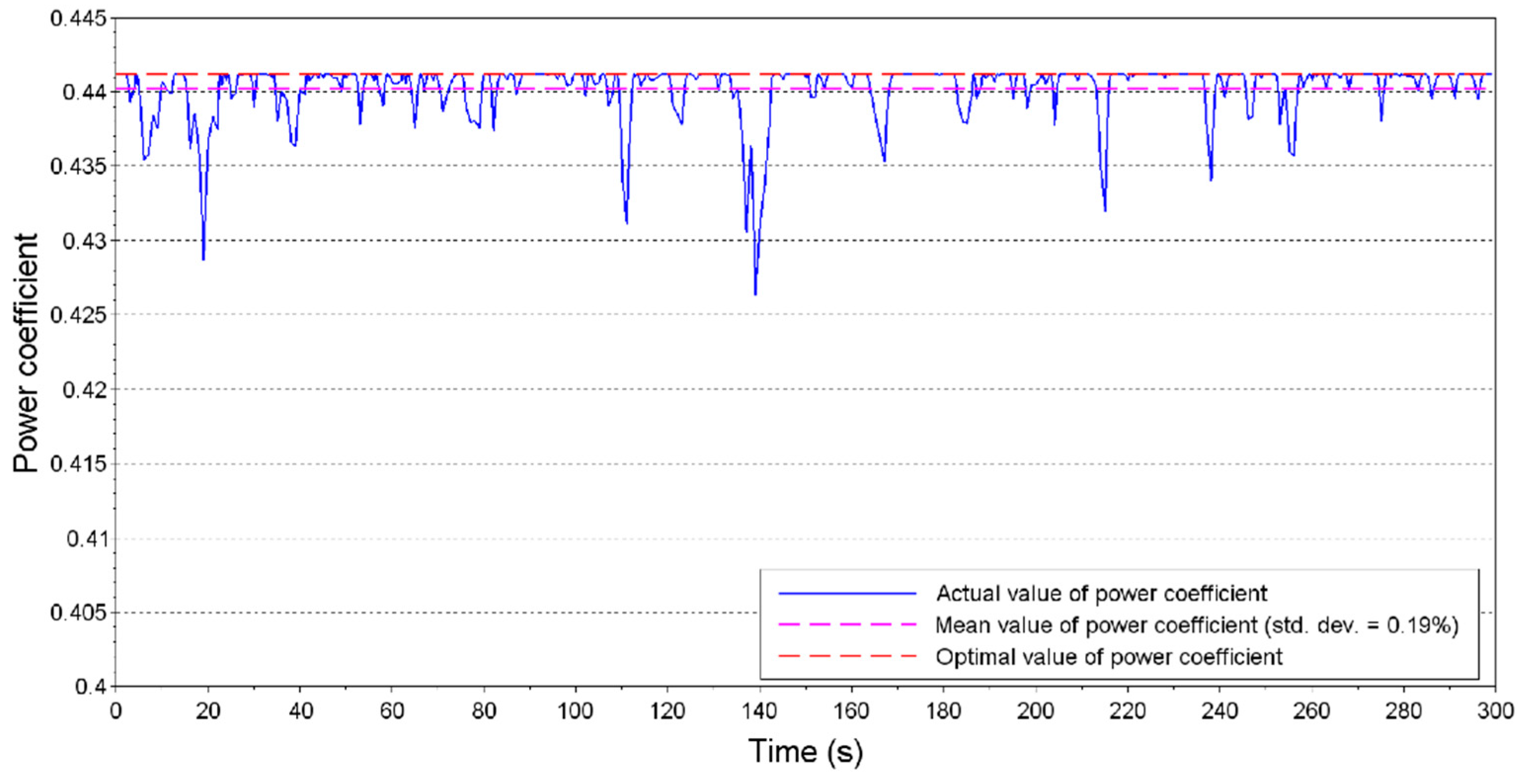
The maximum power extraction from wind occurs when the power coefficient assumes its maximal value, corresponding to β = 0 and λ = λ o t m = 7.206 . To attend this condition, the reference velocity of the DFIG rotor, for different wind velocities, is given by
ω m * = λ o t m V w g b R
In order to maintain the turbine in Maximum Power Point Tracking (MPPT), the angular velocity must be controlled so that the power coefficient is continuously maximal, corresponding to an optimal tip-speed ratio. This must occur from the moment the generator begins to produce power, at a cut-in wind velocity, until the rotor reaches the maximal admitted velocity for the turbine. When this occurs, the control objective is no longer to maintain the optimal tip-speed ratio but to assure the turbine velocity is no higher than the maximal allowed value. This causes a reduction of the power coefficient, reducing the amount of power extracted from the wind. An increase in the wind velocity would lead the turbine to produce more power than the nominal power of DFIG. From this moment on, the pitch control acts on the pitch angle of the blades, so that the absorbed power by the turbine equals the nominal value of DFIG [22,29].
The turbine used in the present work was taken from [29]. Its characteristics are shown in Table 1.

2.2. DFIG Model

The DFIG was modeled by both its steady-state equations and its representation in the direct and quadrature d-q coordinates. Equivalent circuit equations were used to find the rotor steady-state values and to formulate the constrained nonlinear optimization problem, which defines the strategy of evolution of the control variables to their reference value. The DFIG dynamic equations resulting from the d-q reference frame transformation were used to calculate estimated mechanical velocity, rotor currents and magnetizing inductance values. The parameters of the generator used in the simulations can be seen in Table 2 [29].

2.2.1. Equivalent Circuit Equations

In [21,22] the authors demonstrate the steady-state equations in their trigonometric form. In this work, to simplify the algebraic solution of the equation system as well as the restricted nonlinear optimization, the equations are presented in their algebraic form.
The equivalent circuit of DFIG can be seen in Figure 2.
Considering V _ S = V S + j 0 , the complex currents of stator ( I _ S ) and rotor ( I _ R ) , obtained from the equivalent circuit, are
I _ S = V s ( R R + j s X R ) + j V _ R X m ( R s R R s X s X R + s X m 2 ) + j ( R R X s + R s s X R ) ,
I _ R = V _ R ( R S + j X S ) j V s s X m ( R s R R s X s X R + s X m 2 ) + j ( R R X s + R s s X R ) ,
where, R S and X s are the stator resistance and reactance, respectively; s is the slip; R R and X R are the rotor resistance and reactance referred to the stator, respectively; and X m is the magnetizing reactance. The parameters X s and X R are defined as
X S = X l S + X m ,
X R = X l R + X m ,
where, X l S and X l R are the stator and rotor leakage reactances, respectively.
Using Equations (5) and (6), it is possible to calculate the stator and rotor powers, as well the developed power P D . In order to simplify the equations, the variables below are introduced:
A D = ( R s R R s X s X R + s X m 2 ) ,
B D = ( R R X s + R s s X R ) .
The complex powers of stator ( S S ) and rotor ( S R ) are calculated by
S S = 3 V S I S _ * = 3 ( P S + j Q S ) ,
S R = 3 V _ R I _ R * = 3 ( P R + j Q R ) .
Defining V _ R = V R r + j V R i and substituting Equations (5) and (6) in (11) and (12) obtains each power equation (active and reactive) as a function of three variables: slip, real and imaginary parts of the rotor voltage, as presented in Equations (13)–(16).
P S = 3 A D 2 + B D 2 [ V S X m ( B D V R r   A D V R i ) V S 2 ( R R A D + s X R B D ) ] ,
Q S = 3 A D 2 + B D 2 [ V S X m ( A D V R r   B D V R i ) +   V S 2 ( R R B D + s X R A D ) ] ,
P R = 3 A D 2 + B D 2 [ V R r 2 ( R S A D +   X S B D ) + V R i 2 ( R S A D +   X S B D )   V S s X m ( B D V R r + A D V R i ) ] ,
Q R = 3 A D 2 + B D 2 [ V R r 2 ( R S B D   X S A D ) + V R i 2 ( R S B D   X S A D ) +   V S s X m ( A D V R r B D V R i ) ] .
The developed power in the machine is given by [30]
P D = 3 ( 1 s ) s R R I _ R 2 + 3 ( 1 s ) s P R ,
Considering yet
I R 2 = | I _ R | 2 = I _ R I _ R * ,
and, substituting Equation (6) in (18) results in
| I _ R | 2 = ( R S 2 + X S 2 ) ( V R r 2 + V R i 2 ) 2 V S s X S X m V R r 2 V S s X m R S V R i + V S 2 s 2 X m 2 A D 2 + B D 2 .
Finally, the equation for the developed power of a DFIG, in steady state, may be obtained by substitution of Equations (15) and (19) into (17):
P D = 3 ( 1 s ) A D + j B D [ R S X m 2 ( V R r 2 + V R i 2 ) + V S X m ( 2 R R X S B D ) V R r + V S X m ( 2 R S R R A D ) V R i V S 2 s R R X m 2 ]
The stator power may be so calculated, using the energy conservation principle, as
P S = P D + P R P R , l o s s P S , l o s s
where:
P S , l o s s = R S | I S _ | 2
P R , l o s s = R R | I _ R | 2

2.2.2. Dynamic Model of DFIG

The dynamical modeling of DFIG is adopted in the synchronously rotating d-q reference frame, as presented in [28]:
V S d = R S I S d ω e λ S q + d λ S d d t
V S q = R S I S q + ω e λ S d + d λ S q d t
V R d = R R I R d ( ω e P 2 ω m ) λ R q + d λ R d d t
V R q = R R I R q + ( ω e P 2 ω m ) λ R d + d λ R q d t
where ω e is the synchronous electric frequency of the grid; P is the number of poles; R S and R R are the stator and rotor resistances; I S d , I S q , I R d and I R q are the stator and rotor currents; λ S d , λ S q , λ R d and λ R q are the stator and rotor linkage fluxes; V S d , V S q , V R d and V R q are the stator and rotor voltages, respectively. The equations relating currents and fluxes are
λ S d = L S I S d + L m I R d ,
λ S q = L S I S q + L m I R q ,
λ R d = L R I R d + L m I S d ,
λ R q = L R I R q + L m I S q ,
where, L m is the mutual inductance, L S is the stator proper inductance and L R is the rotor proper inductance. Parameters L s and L R are defined as
L S = L l S + L m ,
L R = L l R + L m ,
where, L l S is the stator leakage inductance and L l R is the rotor leakage inductance.
The electromagnetic torque may be given by
T e = 3 2 P 2 ( λ R q I R d λ R d I R q ) ,
and the equation to describe the dynamical behavior of the machine may be expressed using the moment of inertia as
J d ω m d t = T m T e ,
where J is the moment of inertia, whose relationship with the inertia constant H , in seconds, is [31]
J = 2 H ω 0 2 S b ,
where ω 0 is the synchronous velocity in mechanical radians per second and S b is the apparent power in volt-amperes.

2.3. Calculation of Reference Values for Control Variables

The operating point adopted as the basis for the control efficiency study proposed in this article corresponds to the maximum utilization of wind power and unit power factor in the stator. As explained in Section 2.1, for the turbine to extract maximum wind power, the power coefficient must assume the value λ = λ o t m = 7.206 . Therefore, Equation (4) calculates the reference speed and the corresponding reference slip in steady state.
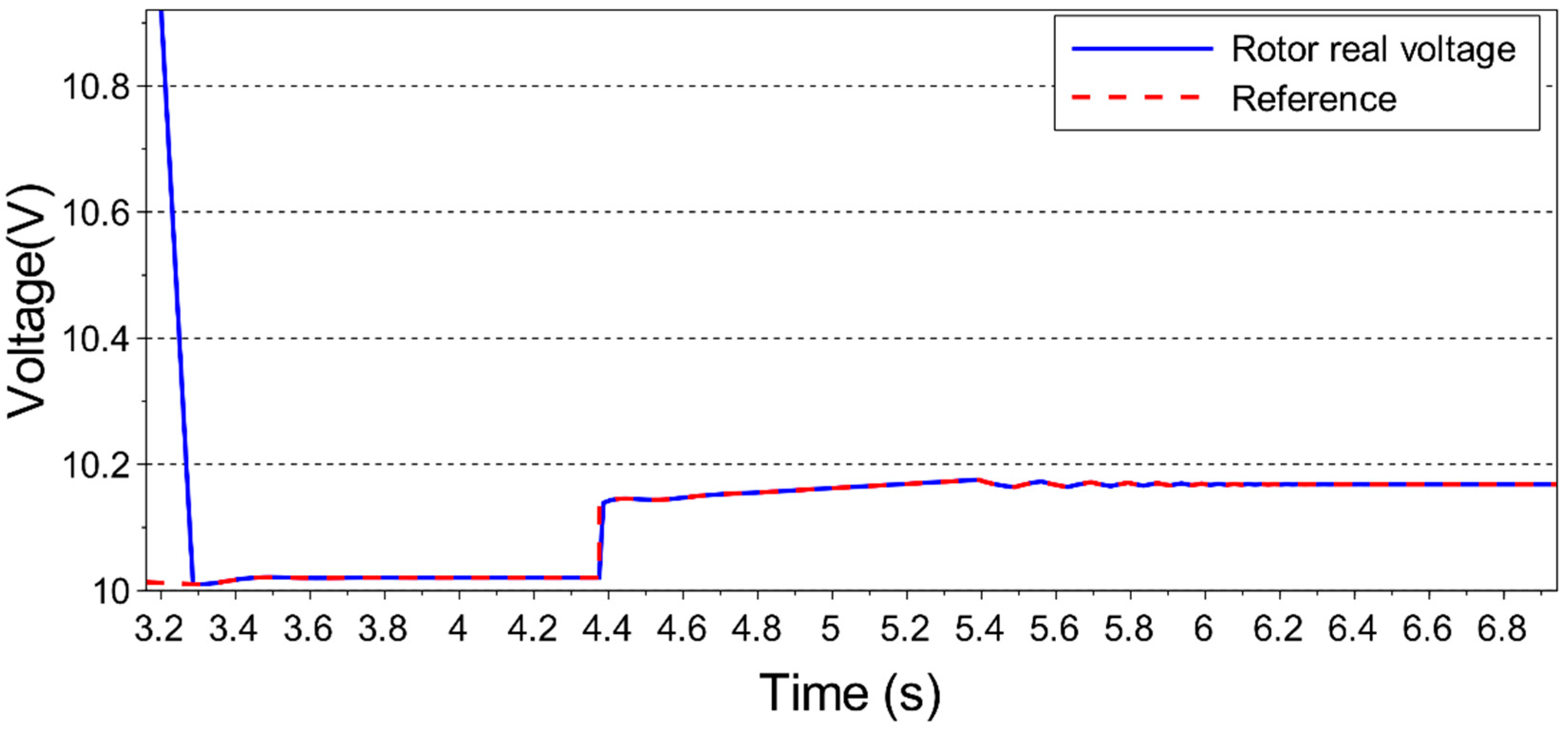
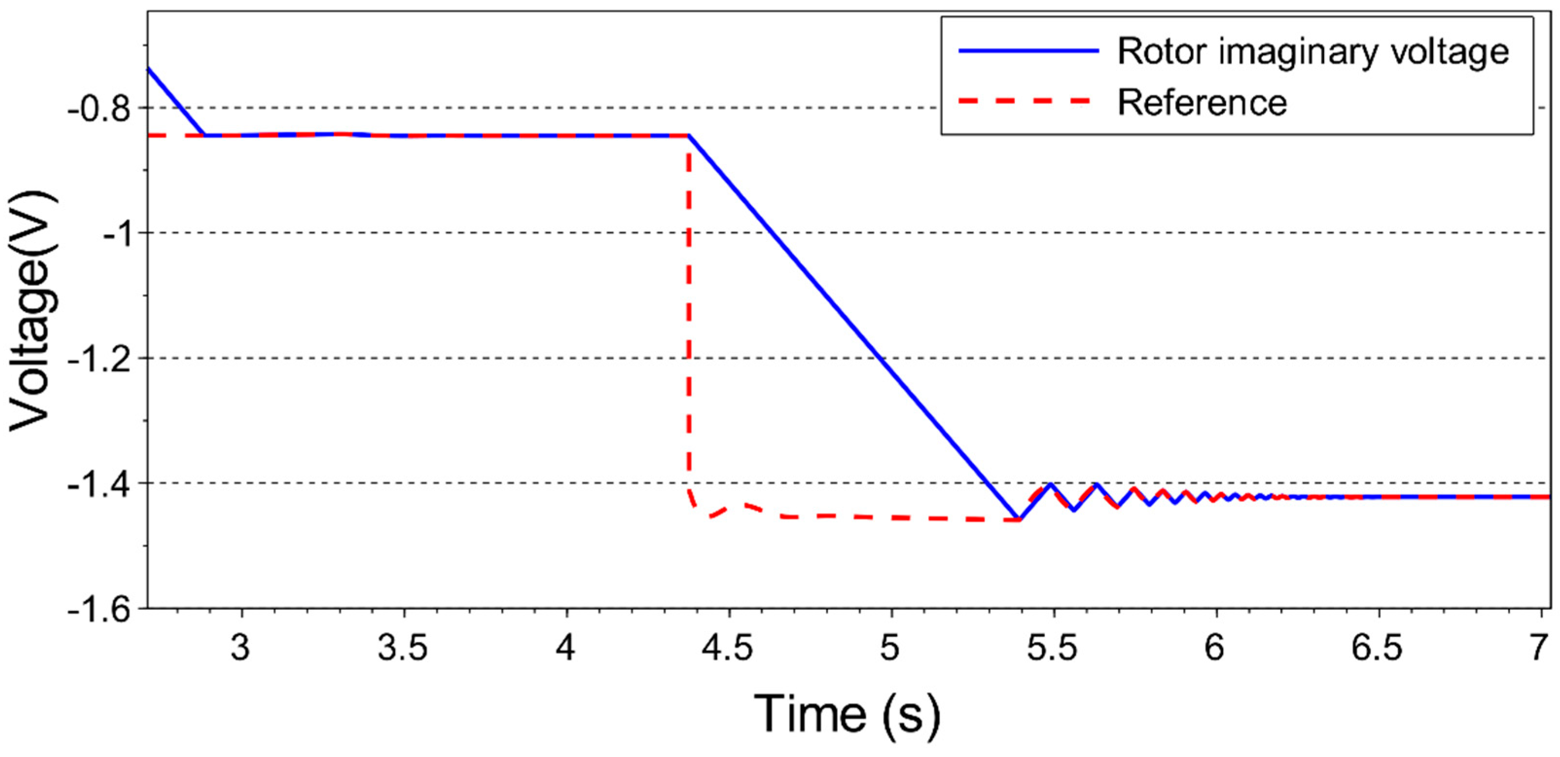
DFIG’s power generation and speed control are done by RSC, which is a voltage source PWM converter. Thus, it is necessary to define the voltage that the converter must supply to the DFIG rotor circuit to control it at the desired operating point. In most studies found in the literature, the rotor reference voltage is given in polar form; in the present work, the reference voltage will be calculated in its Cartesian form. Thus, the rotor reference voltage will have the following form:
V _ R * = V R r * + j V R i *
This way, to keep DFIG operating at the desired operating point, the values of V R r * and V R i * must be known.
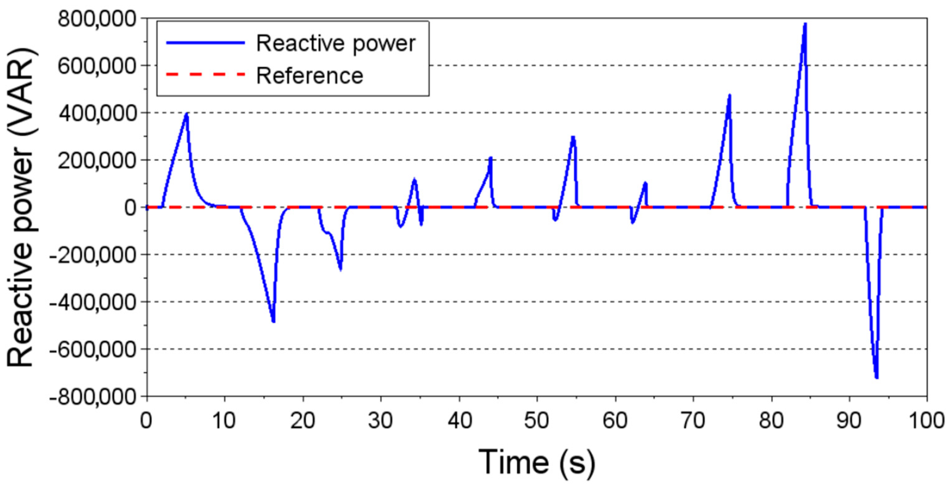
To extract maximum wind power, it is necessary that all mechanical energy absorbed by the turbine be transformed into electrical energy in the generator, disregarding the rotational losses, at the optimal power coefficient value. The second condition imposed on the control is that the stator reactive power is zero. Therefore, the equations system that defines the desired steady-state operating point for the wind turbine is
{ P D = P t Q S = 0
Equations (14) and (20) will form the system proposed in Equation (37) to find the values of V R r * and V R i * that ensures the DFIG will work at the desired operating point in steady state. Thus, the proposed equation system is
{ 3 ( 1 s * ) A D 2 + B D 2 [ R S X m 2 ( V R r * 2 + V R i * 2 ) + V S X m ( 2 R R X S B D ) V R r * + V S X m ( 2 R S R R A D ) V R i *   V S 2 s * R R X m 2 ] P t = 0 V S X m ( A D V R r *   B D V R i * ) +   V S 2 ( R R B D + s * X R A D ) = 0 ,
A D = ( R s R R s * X s X R + s * X m 2 ) ,
B D = ( R R X s + R s s * X R ) .
In addition to the DFIG equivalent circuit parameters, the variables that form the equation system above are the reference slip, s * , which is known for the desired operating point; the stator voltage magnitude ( V S ); and the control variables of RSC, V R r * and V R i * . As can be seen from Figure 1, the stator voltage will vary transiently according to the net current generated by the DFIG. Thus, the use of voltage sensors to measure the amplitude and phase of the stator voltage is necessary for the solution of the equation system.
Having all the data, the system of equations has a simple solution obtained analytically by solving the system defined in Equation (38) (e.g., by variable elimination), thus finding the desired values. Observe that the P D equation has a degree of 2, which results in two solutions. The choice of the appropriate solution is done by analyzing the magnitude of the current corresponding to each of these solutions. The value of the current is calculated by Equation (19), and the solution chosen will correspond to a current smaller than the magnitude of the DFIG rotor-rated current. The solution [ V R r * , V R i * ] is found considering V _ S = V S + j 0 . As shown in the system proposed by Figure 1, the voltage V _ S has a nonzero phase angle, so it is necessary that the actual value of its angle be compensated at the end of the process of calculating the rotor voltage reference values. In the simulations, the stator voltage angle was obtained by the solution of the Thevenin equivalent circuit, but in practice, as it is not possible to know the equivalent of Thevenin at all times, it is necessary to use a Phase-Locked Loop (PLL) algorithm.

2.4. Velocity of the Control Variables Trajectory

The desired operating point is defined by the measured wind velocity, which determines the reference velocity ω m * , according to Equation (4). A change in wind velocity requires new settings of the control variables. The new reference values for these variables, V R r * and V R i * , may be calculated directly by solving Equation (38). Thereafter, a strategy is required for defining the transition from initial steady-state values of these variables ( V R r i and V R i i ) until the corresponding final values ( V R r f and V R i f ), where V R r f = V R r * and V R i f = V R i * . A sudden change of the control variables to their new reference values may cause undesirable or even damaging transients to the network state. For exemplary purposes, a wind velocity step from 7 m/s to 7.5 m/s was simulated, with application of the corresponding rotor voltage step. The resulting rotor current is shown in Figure 3, presenting a transient value high above the rated value.
The current transient caused by application of the rotor voltage step reaches, approximately, two times the rotor nominal current. A current of such magnitude could damage the circuits of the RSC converter. For this reason, the trajectory of control variables towards their reference value must be carefully designed, respecting physical limitations of generator components.
The basic idea of the strategy proposed here is to link the time variations of the control variables, ( d V R r d t and d V R r d t ), to the time variations of the machine speed ( d ω m d t ) in order to define the evolution of the control variables, assuring their convergence compatible to the convergence of the rotor velocity, when steady state is reached. This way, major disturbances are avoided.
Firstly, it will be stated that no overshot in the time response of the rotor velocity is desirable. Thus, this velocity is assumed to change from a previous reference to the next one according to a time-varying exponential function:
ω m = ( ω m i ω m f ) e f ω t + ω m f ,
where, ω m i is the initial value of the velocity, ω m f is its final value ( ω m f = ω m * ) and f ω is a frequency that defines the convergence of the rotor velocity. As the equations from the equivalent circuit presented in Section 2.2.1 contain the variable slip, instead of velocity, a simple relationship between d ω m d t and d s d t can be obtained:
d s d t = d d t ( ω s ω m ω s ) ,
d s d t = 1 ω s d ω m d t ,
Combination of Equations (41) with (43) leads to
d s d t = 1 ω s f ω ( ω m i ω m f ) e f ω t ,
Evaluating Equation (44) in t = 0 gives
[ d s d t ] t = 0 = 1 ω s f ω ( ω m i ω m f ) ,
[ d s d t ] t = 0 = 1 ω s f ω [ ( 1 s i ) ω s ω m f ] ,
Equation (46) may be rearranged as
[ d s d t ] t = 0 = f ω ( s f s i ) .
where s f is the final slip, which must equal the new reference slip s * ; and s i is the initial slip, which could equal the previous reference value, if the machine was previously in a steady state. In order to establish a relationship between the time variations of the control variables with the corresponding slip time variations, Equation (48) is proposed. The basic idea of these equations is to search the aims of maintaining both power conversion and reactive control dynamically.
{ d ( P D P t ) d t = 0 d Q S d t = 0 .
Unlike the system of equations seen in Equation (38), where the reference slip is defined by wind speed, the system of equations proposed here takes into account slip variations that are proportional to the rotor speed variations. Adopting linearization at a time t = t 0 :
d ( P D P t ) d t = ( P D P t ) s d s d t + ( P D P t ) V R r d V R r d t + ( P D P t ) V R i d V R i d t = 0 ,
d Q S d t = Q S s d s d t + Q S V R r d V R r d t + Q S V R i d V R i d t = 0 ,
thus, the equations system is defined by
{ ( P D P t ) s d s d t + ( P D P t ) V R r d V R r d t + ( P D P t ) V R i d V R i d t = 0   Q S s d s d t + Q S V R r d V R r d t + Q S V R i d V R i d t = 0 .
where, the numerical values of the partial derivatives ( P D P t ) V R r , ( P D P t ) V R i , Q S s and Q S V R r as well ( P D P t ) s and Q S s may be calculated at each time t = t 0 using the expressions
( P D P t ) V R r = 3 ( 1 s ) A D 2 + B D 2 [ V S X m ( 2 R R X S B D ) + 2 V R r R S X m 2 ] ,
( P D P t ) V R i = 3 ( 1 s ) A D 2 + B D 2 [ V S X m ( 2 R S R R A D ) + 2 V R i R S X m 2 ] ,
( P D P t ) s = D P D N P D s N P D D P D s D P D 2 ,
where, N P D and D P D are, respectively, the numerator and denominator of the developed power from Equation (20). From Equation (54), the partial derivative of the developed power P D is obtained as a function of slip, s. In this calculation, A D and B D are considered as defined in Equations (9) and (10). Thus, the solution of Equation (54) is
N P D = 3 ( 1 s ) [ R S X m 2 ( V R r 2 + V R i 2 ) + V S X m ( R R X S R S s X R ) V R r       + V S X m ( R S R R + s ( X m 2 + X S X R ) ) V R i   V S 2 s R R X m 2 ] ,
N P D s = 3 [ R S X m 2 ( V R r 2 + V R i 2 ) + V S X m ( R R X S 2 R S s X R ) V R r        + V S X m ( R S R R + 2 s ( X m 2 + X S X R ) ) V R i   2 V S 2 s R R X m 2 ]        + 3 [ V S X m R S X R V R r + V S X m ( X m 2 + X S X R ) V R i V S 2 R R X m 2 ]
D P D = A D 2 + B D 2
D P D s = 2 A D ( X s X R + X m 2 ) + 2 B D R s X R .
The partial derivative expressions of the stator reactive power are as follows:
Q S V R r = 1 A D 2 + B D 2 [ V S X m A D ] ,
Q S V R i = 1 A D 2 + B D 2 [ V S X m B D ] ,
Q S s = D Q S N Q S s N Q S D Q S s D Q S 2 ,
where, N Q S and D Q S are, respectively, the numerator and denominator of the stator reactive power Equation (14). A D and B D are considered as shown in Equations (9) and (10). Thus, the solution of Equation (61) is
N Q S = V S X m [ ( R s R R s X s X R + s X m 2 ) V R r ( R R X s + R s s X R ) V R i ] + V S 2 ( R R 2 X s s 2 X s X R 2 + s 2 X m 2 X R )
N Q S s = V S X m [ ( X s X R + X m 2 ) V R r R s X R V R i ] + V S 2 ( 2 s X s X R 2 + 2 s X m 2 X R )
D Q S = A D 2 + B D 2 .
D Q S s = 2 A D ( X s X R + X m 2 ) + 2 B D R s X R .
After evaluating all partial derivatives and knowing the variables V R r , V R i and s at each instant, the solution of the system of equations proposed in Equation (51) is simply given by
[ d V R r d t d V R i d t ] = [ ( P D P t ) V R r ( P D P t ) V R i Q S V R r Q S V R i ] 1 [ ( P D P t ) s Q S s ] d s d t .
[ d V R r d t d V R i d t ] = [ ξ V r ξ V i ] d s d t
where d s d t is calculated by Equation (47).

2.5. Optimizing Rotor Speed Convergence

Calculation of the convergence speeds of the control variables shown in Equation (66), Section 2.4, depends on the calculation of d s d t . In Equation (47) the variable f ω is responsible for defining the convergence speed of the rotor (mechanical) speed to its reference value, according to the exponential proposed in Equation (41). In order to maximize f ω to lead to a fast convergence of the rotor speed, as well as not violating DFIG limits, a nonlinear constrained optimization technique is proposed in this work. Nonlinear constrained programming problems propose the maximization or minimization and has the following generic form [32]:
{ min f ( x ) ,   x n s . t . { h i ( x ) = 0 ,   i = 1 , , m < n g j ( x ) 0 ,   j = 1 , , p
The problem consists of an objective function f ( x ) , respecting limits imposed by constraint functions, which may be equality h i ( x ) or inequality g j ( x ) . Depending on the proposed problem and the nature of its component functions, different solution techniques may be applied. For the solution of the problem proposed in this work, the Lagrange multiplier method can be applied because it is a relatively simple problem, where the solution of the problem can be found analytically without the need for concern with numerical convergence, as in iterative methods. The first-order condition for the constrained problem using the Lagrange multiplier method is then given by [32].
( x ) = f ( x ) + λ h ( x ) + μ g ( x ) = 0 .
where ( x ) is the Lagrange Augmented Function (Lagrangian) and μ is the Lagrange multiplier.
The optimization problem of variable f ω will be defined as follows for rising wind speed:
{ max f ω ( V R r , V R i ) s . t .   P l i q ( V R r , V R i ) P l i m ,
where f ω can be defined by Equations (34) and (41) for t = 0 as follows:
f ω = T m T e J ( ω m f ω m i ) ,
Torque T m is calculated by Equation (3), and T e is obtained from the developed power equation P D , as shown below:
T e = P D ω m = P D ( 1 s ) ω s ,
T e = 3 [ R S X m 2 ( V R r 2 + V R i 2 ) + V S X m ( 2 R R X S B D ) V R r + V S X m ( 2 R S R R A D ) V R i   V S 2 s R R X m 2 ] ω s ( A D 2 + B D 2 )
The net power is the difference between the stator and the rotor active power, P l i q = P S P R . Thus, from Equations (13) and (15), P l i q is defined as
P l i q = 3 A D 2 + B D 2 [ ( R S A D   +   X S B D ) ( V R r 2 + V R i 2 ) + ( 1 + s ) V S X m B D V R r       + ( 1 + s ) V S X m A D V R i + V S 2 ( R R A D + s X R B D ) ] .
The limitation of the net power generated is justified by the fact that, to produce rotor acceleration, it is necessary that there is a difference between the mechanical torque and the electromagnetic torque, as can be observed by Equation (34). Thus, as the electromagnetic torque is directly proportional to the developed power, as shown in Equation (72), it is necessary to limit the distance of the electromagnetic torque, in order to respect an allowable limit of net power that already discounted the losses in the DFIG. This power limit will be proportional to the available wind power
P l i m = α P t ,
the constant α is chosen by experimental simulations, and it is different for rising or falling wind speed, reflecting operational conditions of the site where the turbine will be installed.
The only constraint proposed in the problem is an inequality constraint, and for the solution of the first-order condition it must be considered active, that is
g ( V R r , V R i ) = P l i q ( V R r , V R i ) P l i m = 0 .
The first-order condition for the optimization problem proposed in Equation (70) is:
( V R r , V R i , μ ) = f ω ( V R r , V R i ) + μ g ( V R r , V R i ) = 0
To find the stationary points of the function presented in Equation (77), it is necessary to assemble the system of equations that define the first-order condition for the Lagrange function and the problem constraint [32], as shown below:
f ω ( V R r , V R i ) = [ f ω V R r f ω V R i ]
g ( V R r , V R i ) = [ g V R r g V R i ]
{ f ω V R r + μ g V R r = 0 f ω V R i + μ g V R i = 0 g ( V R r , V R i ) = 0
where:
f ω V R r = 1 J ( ω m f ω m i ) 3 ω s ( A D 2 + B D 2 ) [ V S X m ( 2 R R X S B D ) + 2 R S X m 2 V R r ]
f ω V R i = 1 J ( ω m f ω m i ) 3 ω s ( A D 2 + B D 2 ) [ V S X m ( 2 R S R R A D ) + 2 R S X m 2 V R i ]
g V R r = 3 ( A D 2 + B D 2 ) [ ( 1 + s ) V S X m B D 2 ( R S A D +   X S B D ) V R r ]
g V R i = 3 ( A D 2 + B D 2 ) [ ( 1 + s ) V S X m A D 2 ( R S A D +   X S B D ) V R i ]
Therefore, System (80) can be rewritten as
{ 1 ω s J ( ω m f ω m i ) [ V S X m ( 2 R R X S B D ) +   2 R S X m 2 V R r ] + μ [ ( 1 + s ) V S X m B D 2 ( R S A D   +   X S B D ) V R r ] = 0 1 ω s J ( ω m f ω m i ) [ V S X m ( 2 R S R R A D ) +   2 R S X m 2 V R i ] + μ [ ( 1 + s ) V S X m A D 2 ( R S A D   +   X S B D ) V R i ] = 0   P l i q ( V R r , V R i ) P l i m = 0
The solution of the system is obtained analytically by manipulating these equations. Dividing the first one by the second leads to
2 V R r [ V S R S X m 3 A D ( 1 + s ) + V S X m ( 2 R S R R A D ) ( R S A D + X S B D ) ]   2 V R i [ V S R S X m 3 B D ( 1 + s ) + V S X m ( 2 R R X S B D ) ( R S A D + X S B D ) ]   = V S 2 X m 2 B D ( 2 R S R R A D ) ( 1 + s ) + V S 2 X m 2 A D ( 2 R R X S B D ) ( 1 s )
Thus, the Lagrange multiplier is eliminated, and an equation is obtained from which it is possible to explicit V R r as a function of V R i . Entering the following constants:
K V r = 2 [ V S R S X m 3 A D ( 1 + s ) + V S X m ( 2 R S R R A D ) ( R S A D +   X S B D ) ] ,
K V i = 2 [ V S R S X m 3 B D ( 1 + s ) + V S X m ( 2 R R X S B D ) ( R S A D +   X S B D ) ] ,
K i = V S 2 X m 2 B D ( 2 R S R R A D ) ( 1 + s ) + V S 2 X m 2 A D ( 2 R R X S B D ) ( 1 s ) ,
one obtains
V R r = K V i V R i + K i K V r .
Substitution of Equation (90) in constraint g ( V R r , V R i ) leads to
[ ( R S A D +   X S B D ) ( ( K V i V R i + K i K V r ) 2 + V R i 2 ) + ( 1 + s ) V S X m B D ( K V i V R i + K i K V r )         + ( 1 + s ) V S X m A D V R i + V S 2 ( R R A D + s X R B D ) ] P l i m A D 2 + B D 2 3 = 0
This polynomial has two roots, which represent two possible solutions for V R i o t m . Replacing these solutions into Equation (90), yields two solution pairs [ V R r o t m , V R i o t m ], known as stationary (or critical) points of the problem.
The first analysis of the critical points is done by observing the signal of the Lagrange multiplier μ , calculated by the following equation, taken from the system presented in Equation (85):
μ = 1 ω s J ( ω m f ω m i ) [ V S X m ( 2 R R X S B D ) + 2 R S X m 2 V R r o t m ( 1 + s ) V S X m B D 2 ( R S A D +   X S B D ) V R r o t m ] ,
When the constraint is of inequality type, the sign of the Lagrange multiplier expresses the need to use the imposed constraint to limit the objective function. If the problem is maximization and the inequality constraint is of type “greater or equal”, a positive sign of the multiplier indicates that the constraint is naturally limiting the objective function because its gradients are opposite to ensure the first-order condition seen in Equation (77). If the problem is minimization, with the inequality constraint of type “less than or equal”, a negative sign of the Lagrange multiplier leads to the same conclusion. When, in the cases presented, the signs are opposite, it means that the objective function is being forced to go to the constraint limit, in which case it would be unwanted.
After applying the first-order condition and calculating the critical points, it is necessary to analyze the second-order condition and the Hessian matrix of the problem. The second-order condition is applied as shown below:
2 ( V R r , V R i , μ ) = 2 f ω ( V R r , V R i ) + μ 2 g ( V R r , V R i ) ,
and the Hessian matrix is presented below:
H = [ ω I 2 ( V R r o t m , V R i o t m ) g ( V R r o t m , V R i o t m ) T g ( V R r o t m , V R i o t m ) 0 ] .
The analysis of the eigenvalues of the Hessian matrix is necessary to define the convexity of the region around each critical point and to verify if they are minimum or maximum points [31]. The eigenvalues are obtained from the Hessian determinant as shown below:
d e t [ ω 2 ( V R r o t m , V R i o t m ) V R r 2 2 ( V R r o t m , V R i o t m ) V R r V R i g ( V R r o t m , V R i o t m ) V R r 2 ( V R r o t m , V R i o t m ) V R i V R r ω 2 ( V R r o t m , V R i o t m ) V R i 2 g ( V R r o t m , V R i o t m ) V R i g ( V R r o t m , V R i o t m ) V R r g ( V R r o t m , V R i o t m ) V R i    0 ] = 0
If all the eigenvalues of the Hessian matrix, analyzed for a certain critical point, have a positive sign, then the region around the critical point is convex; therefore, this is a minimum. If negative, the critical point is a maximum of the objective function [32].
The objective function and the constraint function of the problem proposed by Equation (70) are both second-order polynomials. Thus, it is expected that the critical points found are one maximum and one minimum. Therefore, the critical point that solves this problem will be one that maximizes the objective function. Similarly, when the wind is decreasing, the problem becomes minimization, as shown below:
{ min f ω ( V R r , V R i ) s . t .   P l i q ( V R r , V R i ) P l i m ,
All mathematical inferences presented throughout this section are valid for this formulation as well.
In the second-order condition, for the problem presented in Equation (70), we search for the critical point that generates the eigenvalue of the Hessian matrix, with negative sign, which maximizes the objective function. For the problem presented in Equation (96) the eigenvalue of the Hessian matrix should be positive.
At the end of the optimization process of f ω , we arrive at a pair V R r o t m and V R i o t m . Therefore,
f ω o t m = T m T e ( V R i o t m , V R i o t m ) J ( ω m f ω m i ) .
and
d s d t o t m = f ω o t m ( s f s i ) .
The optimal values of the derivatives of the control variables V R r and V R i at t = 0 are determined from Equations (67) and (98).
[ d V R r d t o t m d V R i d t o t m ] = [ ξ V r ξ V i ] d s d t o t m
As for the rotor speed, the exponential behavior for the convergence of control variables was also adopted. Therefore, generally,
V R r = ( V R r i V R r f ) e f v r t + V R r f ,
V R i = ( V R i i V R i f ) e f v i t + V R i f ,
where, f v r and f v i are the frequencies that define the convergence velocity, and V R r f and V R i f are the final values of the control variables (i.e., their reference values).
To find the optimal convergence frequencies f v r and f v i , a relationship to the optimal velocity convergence frequency is established. Deriving V R r and V R i :
d V R r d t = f v r ( V R r i V R r f ) e f v r t
d V R i d t = f v i ( V R i i V R i f ) e f v i t
Substituting Equations (102) and (103) into Equation (99) gives
f v r o t m ( V R r i V R r f ) e f v r o t m t = ξ V r d s d t o t m
f v i o t m ( V R i i V R i f ) e f v i o t m t = ξ V i d s d t o t m
Substituting Equation (98) into Equations (104) and (105) and analyzing them at t = 0 , one concludes
f v r o t m = ξ V r f ω o t m ( s f s i ) ( V R r i V R r f )
f v i o t m = ξ V i f ω o t m ( s f s i ) ( V R i i V R i f )

2.6. Speed Estimation and Magnetizing Inductance Correction

Magnetic saturation affects the inductance value of the DFIG, and consequently the control performance [23]. However, the effect of this saturation mainly influences the magnetizing inductance since the path of the magnetic leakage flux is mainly air; thus, the variations of the leakage inductances are irrelevant to the control [24]. Changes in inductance values may lead to a different operating point than expected. Still, considering that the magnetizing inductance is the parameter that has the highest value, compared to the other DFIG parameters, it is important to identify its value to ensure control efficiency. Because of these facts, a strategy is proposed here for estimating the value of the magnetizing inductance by means of measuring stator voltages and currents and estimating rotor slip and rotor currents. The proposed procedure considers that the identification of magnetizing inductance should not necessarily be performed at each step of the control. An error in its value would lead the DFIG to an erroneous steady-state operating point. This way, correction of the magnetizing inductance value should be performed when detecting the achievement of this condition, with differences in the expected values for variables such as, for example, reactive power. For this reason, the proposed strategy is based on the dynamic equations of DFIG, considering that, for steady state, one has d λ d t = 0 . It is assumed that the d axis of the Park transform is aligned with the stator voltage, which means that V S d = V S and V S q = 0 , where V S d and V S q are the stator voltages at the d and q coordinates. From these considerations and from Equations (27) to (34), the problem can be solved as follows:
V S d = R S I S d ω e ( L S I S q +   L m I R q ) ,
0 = R S I S q + ω e ( L S I S d +   L m I R d ) ,
V R d = R R I R d s ω e ( L R I R q   L m I S q ) ,
V R q = R R I R q + s ω e ( L R I R d   L m I S d ) .
It should be noted that Equations (27) to (34) assume that the directions of stator and rotor currents are entering the DFIG. The stator current direction assumed for the mathematical equation of the strategy proposed here, as shown in Figure 2, comes out of the generator, so the stator current signals have been changed to suit the calculation.
From Equations (108) and (109), the value of the rotor currents can be estimated as follows:
I ˜ R d = R S I ^ S q + ω e L ˜ S I ^ S d ω e L ˜ m
I ˜ R q = V ^ S d R S I ^ S d + ω e L ˜ S I ^ S q ω e L ˜ m
The values of the variables represented with “~” are estimated, whereas the variables represented with “^” have their values measured. Therefore, I ˜ R d and I ˜ R q are the estimated values of rotor currents, and V ^ S d , V ^ S q , I ^ S d and I ^ S q are the measured values of stator voltages and currents, respectively. L ˜ m and L ˜ S are the estimated values of the magnetizing inductance and stator self-inductance, respectively. Initially, their nominal values are considered for the calculation.
As previously mentioned, variations in the dispersion inductances are irrelevant in the control, so it is possible to state that variations in the DFIG magnetizing inductance are reflected in equal proportions in the rotor and stator proper inductances, as follows:
L m L ˜ m = L S L ˜ S
where L m and L S are the nominal values provided by the manufacturer. Substituting Equation (31) into (114) results in
L l S + L m L m = L ˜ S L ˜ m
( 1 + k l S ) L ˜ m = L ˜ S
where,
k l S = L l S L m
Similarly to the rotor:
( 1 + k l R ) L ˜ m = L ˜ R
k l R = L l R L m
and, therefore, it is possible to modify Equations (112) and (113) to be exclusively dependent on L ˜ m ,
I ˜ R d = R S I ^ S q + ω e ( 1 + k l S ) L ˜ m I ^ S d ω e L ˜ m ,
I ˜ R q = V ^ S d R S I ^ S d + ω e ( 1 + k l S ) L ˜ m I ^ S q ω e L ˜ m .
With the estimated values of rotor currents by Equations (120) and (121), it is possible to estimate the slip and magnetizing inductance by Equations (110) and (111), respectively, as shown below:
s ˜ = V R d + R R I ˜ R d ω e ( ( 1 + k l R ) L ˜ m I ˜ R q L ˜ m I ^ S q ) ,
L ˜ m 2 [ s ˜ ω e 2 I ^ S d   s ˜ ω e 2 ( 1 + k l r ) ( 1 + k l s ) I ^ S d ]    + L ˜ m [ ω e V R q ω e R R ( 1 + k l s ) I ^ S q s ˜ ω e ( 1 + k l r ) R S I ^ S q ] + R R ( V ^ S d    + R S I ^ S d ) = 0 ,
and the values of V R d and V R q are found by Equations (100) and (101).
The slip estimation process is performed in real time, and its estimated value is used in the optimization process presented in Section 2.4 and Section 2.5. The estimation of magnetizing inductance is not performed in real time, as the current transient would generate unrealistic values for L ˜ m . The strategy proposes that the magnetizing inductance value should be calculated when the machine is in a steady state and the stator reactive power is not close to zero, considering a tolerance. Failure to achieve this objective of steady-state control indicates that the value of the magnetizing inductance used in calculating the reference values of the control variables is different from the actual value. It is expected that, under this condition, the estimated rotor and slip current values are wrong. Upon detecting this condition, the value of L ˜ m will be corrected using Equation (123), and the corrected value will be used for the calculation of the analytic solution and optimal strategy routines.
There are two values for L ˜ m possible for the solution of Equation (123). To achieve a less turbulent convergence toward the actual inductance value, the value closest to the value calculated in the previous step is always chosen.

3. Results

The DFIG RSC control methodology proposed in this article was analyzed by applying wind speed steps, as shown in Figure 4. This wind profile was adopted with the intention of demonstrating the effectiveness of the proposed method in low and high wind speeds, as well as near zero slip. The wind speed ranging from 5.5 to 10.0 m/s was adopted to respect the generator speed limits presented in Table 2, corresponding to a slip range of 30% to −30%, approximately. In order to ensure that the control assumptions are respected, the convergence of velocity to its reference value should be analyzed, as well as the behavior of the control variables.
For each wind speed, a reference rotor speed for the maximum wind power extraction was defined, as shown in Equation (4). The control variables V R r and V R i had their reference values calculated over time by Equation (38) and changed due to stator voltage variation, caused by transitory currents. The exponentials presented in Equations (100) and (101) defined the trajectory of V R r and V R i to their reference values. Figure 5 and Figure 6 show this behavior.
The optimization process was proposed to define an optimal rotor convergency speed and, by this, to calculate a trajectory for the control variables that respects some power limits. The strategy intended to accelerate the DFIG rotor by maintaining a difference between the mechanical torque and the electromagnetic torque, and this difference depended on the value that was chosen for the constant α , as shown at Equation (75). The value of α has been set to 0.85 for rising speed wind and at 1.15 for falling speed wind, and the effect of this strategy can be observed by the torques in Figure 7.
For the effect of the distance between the torques, the DFIG rotor accelerated or deaccelerated to reach the speed corresponding to the maximum power extraction point operation. Figure 9 shows the rotor speed behavior and its convergence to the reference values. The value of the estimated rotor speed was accurate, and the difference between both curves can hardly be observed in Figure 8.
To verify the effectiveness of the proposed strategy at steady state, the developed, active and wind powers were analyzed. The behavior of the torques directly influenced the active power output, as can be analyzed from Figure 9.
The net active power moved away from its previous value, increasing or decreasing, because of the behavior of the electromagnetic torque, but it quickly converged to its steady-state value. The developed power had a similar behavior, and transiently, the value of λ was not optimal. At convergence, the value of the developed power was equal to the value of the power delivered by the wind. Net active power was lower due to stator and rotor losses.
Similar to net active power, due to machine acceleration, the value of stator reactive power did not remain constant, as can be seen from Figure 10.
Since there was no voltage control, transient reactive power variations caused variations in stator voltage. Despite the reactive power peaks, the stator voltage remained within the limits imposed by the international grid codes, transiently [33], as shown in Figure 11.
The slip estimation strategy based on the rotor current estimation, using only the stator variables, proved to be efficient and accurate, as shown in Figure 8. In order to analyze the algorithm to correct the value of the magnetizing inductance online, the following situation was supposed. The value of this parameter, used to solve the Runge–Kutta method, was changed to 70% of its nominal value. Thus, control algorithms (composed of analytical solutions to the control variables), the optimal strategy for rotor speed convergency and estimation of the rotor currents and slip all became dependent on a value of the magnetizing inductance that was different from the real value at the DFIG. Since its value was corrected only in a steady-state situation, the control will perform transiently and give wrong information. To test the algorithm, a variation of wind speed from 7.5 to 8 m/s was used, and the result is shown in Figure 12.
As should be expected, there was an error between the actual rotor speed and its estimated value, caused by the wrong value of the magnetizing inductance. In addition, the rotor speed would not converge to its optimal reference value, since the reference values for the control variables were miscalculated. As can be observed in Figure 13, the first convergence value, approximately between 3.3 and 4.4 s, was very close to the optimal value. This means the tip-speed ratio was near its optimal value, and the effect of the wrong value of the magnetizing inductance had a small effect on tracking the maximum power point; however, the value of the reactive power at the stator was significantly affected, as shown in Figure 13. Between 3.3 and 4.4 s the reactive power consumed from the grid was about 280 kvar.
At 4.4 s, the proposed algorithm to correct the value of magnetizing inductance started. This algorithm rapidly converged to a value very close to the real one. The control variables were quickly corrected too, as shown in Figure 14, Figure 15 and Figure 16. Then, the rotor speed and the stator reactive power converged to its desired value, as shown in Figure 12 and Figure 13.
In order to test the proposed control in situations near to real conditions, a set of real measurement data of wind speed in a real farm was obtained. A selected range of 10 min, characterized by the mean value and standard deviation, was used to compose 600 points following a normal distribution. This variation is presented in Figure 17.
Observe that the variations incorporated ascendant and descendant ramps, differently from the previous simulations. The resulting speeds obtained by applying the new control strategy are sketched in Figure 18. Once more, the estimated rotor speed superposed the real speed, attesting the efficiency of the rotor speed estimation.
The efficiency of extracting power from wind may be evaluated by calculating the total optimal energy available and the total energy converted for the period considered in Figure 18, as suggested by [15]. Proceeding this way, the obtained value was about 98%, which was 5% higher than the best result presented in that reference. However, it is important to point out that different wind speed profiles were used in both simulations; the wind speed profile of Figure 17 better reflected the wind behavior from the specific site where the measurement data were obtained. The corresponding voltages were such that the difference between the maximal and minimal voltages by this simulation corresponded to a range of about 0.5%. No violations in variable limits were detected.
In order to give another idea about the efficiency of the proposed control strategy, the variation of the power coefficient with time is sketched in Figure 19. In this figure, a comparison between the optimal value, the mean value and the actual value of the power coefficient was registered for a time period of 300 s. The mean value corresponded to 99.77% of the optimal value, with a standard deviation of 0.19%.

4. Discussion

In previous works, objectives are set, and the control variables match their final values by approximation as objectives are achieved. In the present work, final values of the control variables (references) are calculated by means of an analytical procedure to solve a system of nonlinear equations. If the terminal voltage cannot be considered constant because of high equivalent Thévenin impedance, the reference rotor voltages must be recalculated using information acquired from a voltage sensor and a PLL.
A new DFIG control strategy was proposed and presented using a nonlinear, real-time optimization process, formulated from the equivalent circuit equations. In addition, a solution for the machine slip estimation and magnetizing inductance estimation for online correction of values was presented. The proposed control strategy performed the DFIG rotor acceleration optimally, respecting the limits of net power injected into the grid, by means of controlling the trajectory of the control variables that defined the RSC voltage. The electromagnetic and mechanical torques moved apart for a brief period to cause acceleration of the rotor, which caused the injected net power to rise or fall for a few seconds. Control has proven to be effective over a wide range of wind speeds, and the only parameter to be defined, in order to reach this purpose, was the net active power limit. Rotor currents were transiently controlled well, and reactive power peaks caused mild overvoltages or undervoltages well below the limits imposed by actual regulations. The strategy to estimate rotor currents, slip and the magnetizing inductance obtained from the dynamical formulation of DFIG has proven to be effective. It used only stator voltage and current sensors, being independent of rotor and speed sensors, thus reducing the number of sensors in the system. Table 3 presents a synthetic comparation of the Direct Voltage Control (DVC), here proposed, with other methods found in the literature.

5. Conclusions

The major objective of the present work was to control a DFIG efficiently, without relying on parameters that can be corrupted over time like PI gains. An optimization process was proposed to define an optimal rotor convergency speed and thus define the trajectory of the control variables, respecting some power limits. The strategy intended to accelerate the DFIG rotor by maintaining a difference between the mechanical torque and the electromagnetic torque, and this difference depended on the allowed limit in net active power. This limit defines the momentaneous acceleration of the machine, in response to wind speed variations. When the wind speed changes, a new mechanical torque is imposed. The difference to the instantaneous electromagnetic torque, resulting in the acceleration torque, may not be enough to cause a fast convergence to the new reference speed. This way, the objective of optimization was to maximize acceleration, respecting limits on other variables.
Implementation of the optimization process is dependent on the instantaneous values of rotor speed. In order to avoid the necessity of using a speed sensor, a process of rotor speed estimation was proposed. As presented in Figure 8, the estimated speed resulted very close to the actual rotor speed, obtained by solving the differential equation set.
Simulation results demonstrated that too high acceleration torques (or powers) may cause violations both in currents or in voltage limits (see Figure 3). This way, optimization had to be constrained. This was implemented by limiting the net generated active power as a percentage of the previous reference power. For both wind speed profiles used (step change and near to real conditions) as example in this article, a variation of ±15% was adjusted so that no violations in currents or voltages magnitudes could have resulted. Considering all simulations, the highest resulting voltage amplitude was about 1.5% above the nominal value, as shown in Figure 11.
From the results of simulations performed for a real wind speed profile, it was observed (see Figure 18) that the proposed control was efficient in keeping the rotor speed close to the reference speed. Furthermore, the time variation of the power coefficient, as shown in Figure 19, presented an average very close to the optimal value.
Variations in the magnetizing inductance value have been shown to cause DFIG to operate at a different operating point than desired, implying small errors in rotor steady state velocity but a significant error in reactive power. The proposed algorithm quickly detected errors in the magnetizing inductance and corrected its value with good precision, causing the generator to work as expected, according to the right trajectory of control. The main advantages of the proposed method can be observed by comparing it other methods with respect to some desired features, as compiled in Table 3. From this table, it can be observed (third and fifth columns) that requiring fast convergence leads to a compromise in active power flow. It must be pointed out that oscillations in power flow may cause voltage fluctuations and, therefore, should be avoided. In general, the DFIG Direct Voltage Control with an optimum rotor acceleration strategy and parameter estimation proved to be effective in reaching the proposed objectives. The proposed technique is planned to be checked in an experimental system in a further work.

Author Contributions

Conceptualization, A.M. and M.F.M.J.; Data curation, A.M.; Formal analysis, A.M., J.T.d.O. and M.F.M.J.; Investigation, A.M., T.R., J.T.d.O. and M.F.M.J.; Methodology, A.M., T.R., J.T.d.O. and M.F.M.J.; Project administration, M.F.M.J.; Software, A.M. and T.R.; Supervision, M.F.M.J.; Visualization, A.M. and T.R.; Writing—original draft, A.M.; Writing—review & editing, T.R. and M.F.M.J. All authors have read and agreed to the published version of the manuscript.

Funding

This research received no external funding.

Conflicts of Interest

The authors declare no conflict of interest.

References

  1. Yaramasu, V.; Wu, B.; Sen, P.C.; Kouro, S.; Narimani, M. High-Power Wind Energy Conversion Systems: State-of-the-Art and Emerging Technologies. Proc. IEEE 2015, 5, 103. [Google Scholar] [CrossRef]
  2. Ramos, T.; Medeiros Júnior, M.F.; Pinheiro, R.; Medeiros, A. Slip Controlo of a Squirrel Cage Induction Generator Driven by an Eletromagnetic Frequency Regulator to Achieve the Maximum Power Point Tracking. Energies 2019, 12, 2100. [Google Scholar] [CrossRef] [Green Version]
  3. You, R.; Barahona, B.; Chai, J.; Cutululis, N.A. A Novel Wind Turbine Concept Based on an Electromagnetic Coupler and the Study of Its Fault Ride-through Capability. Energies 2013, 6, 6120–6136. [Google Scholar] [CrossRef] [Green Version]
  4. Martinez, M.I.; Tapia, G.; Susperregui, A.; Camblong, H. Sliding-Mode Control for DFIG Rotor and Grid-Side Converters Under Unbalanced and Harmonically Distorted Grid Voltage. IEEE Trans. Energy Conv. 2012, 27, 328–339. [Google Scholar] [CrossRef]
  5. Pena, R.; Clare, J.C.; Asher, G.M. Doubly fed induction generator using back-to-back PWM converters and its application to variable-speed wind-energy genetration. IEEE Proc. Electr. Power Appl. 1996, 143, 231–241. [Google Scholar] [CrossRef] [Green Version]
  6. Li, S.; Haskew, T.A.; Williams, K.A.; Swatloski, R.P. Control of DFIG With Turbine Direct-Current Vector Control Configuration. IEEE Trans. Sust. Energy 2012, 3, 1–11. [Google Scholar] [CrossRef]
  7. Nunes, M.V.A.; Lopes, J.A.P.; Zürn, H.H.; Bezerra, U.H.; Almeida, R.G. Influence of the Variable-Speed Wind Generators in Transient Stability of the Conventional Generators Integrated in Electrical Grids. IEEE Trans. Energy Conv. 2004, 19, 692–701. [Google Scholar] [CrossRef] [Green Version]
  8. Prajapat, G.P.; Senroy, N.; Kar, I.N. Modified Control of DFIG-WT for the Smooth Generator Speed Response under Turbulent Wind. In Proceedings of the 14th IEEE India Council International Conference (INDICON), Roorkee, India, 15–17 December 2017. [Google Scholar]
  9. Setiawan, I.; Facta, M.; Priyadi, A.; Purnomo, M.H. Analysis and Comparison of Control Strategies for a DFIG-Small Wind Turbine System with High Fluctuating Wind Speed Conditions. IREE Intern. Rev. Elect. Eng. 2017, 12, 110–120. [Google Scholar] [CrossRef]
  10. Kharchouf, I.; Essadki, A.; Arbaoui, M.; Nasser, T. Modeling and PI Control Strategy of DFIG Based Wind Energy Conversion Systems. In Proceedings of the 2017 International Renewable and Sustainable Energy Conference (IRSEC), Tangier, Morocco, 4–7 December 2017. [Google Scholar]
  11. Mohseni, M.; Islam, S.M.; Masoum, M.A.S. Enhanced Hysteresis-Based Current Regulators in Vector Control of DFIG Wind Turbines. IEEE Trans. Power Eletr. 2011, 26, 223–234. [Google Scholar] [CrossRef]
  12. Takahashi, I.; Noguchi, T. A New Quick-Response and High-Efficiency Control Strategy of Induction Motor. IEEE Trans. Ind. Appl. 1986, IA-22, 820–827. [Google Scholar] [CrossRef]
  13. Yousefi-Talouki, A.; Zalzar, S.; Pouresmaeil, E. Direct Power Control of Matrix Converter-Fed DFIG with Fixed Switching Frequency. Sustainability 2019, 11, 2604. [Google Scholar] [CrossRef] [Green Version]
  14. Xu, L.; Cartwright, P. Direct Active and Reactive Power Control of DFIG for Wind Energy Generation. IEEE Trans. Energy Conv. 2006, 21, 750–758. [Google Scholar] [CrossRef]
  15. Bektache, A.; Boukhezzar, B. Nonlinear predictive control of a DFIG-based wind turbine for power capture optimization. Int. J. Electr. Power Energy Sys. 2018, 101, 92–102. [Google Scholar] [CrossRef]
  16. Sguarezi Filho, A.; de Oliveira, A.L.; Rodrigues, L.L.; Costa, E.C.M.; Jacomini, R.V. A Robust Finite Control Set Applied to the DFIG Power Control. IEEE J. Emerg. Sel. Topics Power Eletr. 2018, 6, 1692–1698. [Google Scholar] [CrossRef]
  17. Sun, D.; Wang, X.; Nian, H.; Zhu, Z.Q. A Sliding-Mode Direct Power Control Strategy for DFIG Under Both Balanced and Unbalanced Grid Conditions Using Extended Active Power. IEEE Trans. Power Eletr. 2018, 33, 1313–1322. [Google Scholar] [CrossRef]
  18. Mohammadi, J.; Vaez-Zadeh, S.; Afsharnia, S.; Daryabeigi, E. A Combined Vector and Direct Power Control for DFIG-Based Wind Turbines. IEEE Trans. Sust. Energy 2014, 5, 767–775. [Google Scholar] [CrossRef]
  19. Soued, S.; Ramadan, H.S.; Becherif, M. Dynamic Behavior Analysis for Optimaly Tuned On-Grid DFIG Systems. Energy Proc. 2019, 162, 339–348. [Google Scholar] [CrossRef]
  20. Alhato, M.M.; Bouallègue, S. Direct Power Control Optimization for Doubly Fed Induction Generator Based Wind Turbine Systems. Math. Comput. Appl. 2019, 24, 77. [Google Scholar] [CrossRef] [Green Version]
  21. Liu, C.; Hsu, Y. Effect Effect of Rotor Excitation Voltage on Steady-State Stability and Maximum Output Power of a Doubly Fed Induction Generator. IEEE Trans. Ind. Electron. 2011, 58, 1096–1109. [Google Scholar] [CrossRef]
  22. Aguglia, D.; Viarouge, P.; Wamkeue, R.; Cros, J. Analytical determination of steady-state converter control laws for wind turbines equipped with doubly fed induction generators. IET Renew. Power Gen. 2008, 2, 16–25. [Google Scholar] [CrossRef]
  23. Djoudi, A.; Chekireb, H.; Berkouk, E.; Bacha, S. Real Time Estimation of DFIG Inductances and Rotor Currents. In Proceedings of the 3rd Renewable Power Generation Conference (RPG 2014), Naples, Italy, 24–25 July 2014; pp. 1–5. [Google Scholar]
  24. Zhi, S.; Xu, L. Direct Power Control of DFIG With Constant Switching Frequency and Improved Transient Performance. IEEE Trans. Energy Conv. 2007, 22, 110–118. [Google Scholar] [CrossRef]
  25. Prasad, R.M.; Mulla, M.A. A Novel Position-Sensorless Algorithm for Field-Oriented Control of DFIG With Reduced Current Sensors. IEEE Trans. Sust. Energy 2019, 10, 1098–1108. [Google Scholar] [CrossRef]
  26. Singh, B.; Naidu, N.K.S. Direct Power Control of Single VSC-Based DFIG Without Rotor Position Sensor. IEEE Trans. Ind. Appl. 2014, 50, 4152–4163. [Google Scholar] [CrossRef]
  27. Lubosny, Z. Wind Turbine Operation in Electric Power Systems; Springer: Berlin/Heidelberg, Germany, 2010; ISBN 978-3-642-07317-5. [Google Scholar]
  28. Tanvir, A.A.; Merabet, A.; Beguenane, R. Real-Time Control of Active and Reactive Power for Doubly Fed Induction Generator (DFIG)-Based Wind Energy Conversion System. Energies 2015, 8, 10389–10408. [Google Scholar] [CrossRef] [Green Version]
  29. Slootweg, J.G. Wind Power: Modelling and Impact on Power System Dynamics. Ph.D. Thesis, Technische Universiteit Delft, Delft, The Netherlands, 2003. [Google Scholar]
  30. Sharkawi, M.A.E. Overview of Wind Turbines. In Wind Energy: An Introduction, 1st ed.; CRC Press: New York, NY, USA, 2016; ISBN 978-1-4822-6400-5. [Google Scholar]
  31. Kundur, P. Power System Stability and Control; McGraw-Hill: New York, NY, USA, 1994; ISBN 0-07-035958-X. [Google Scholar]
  32. Luemberger, D.G.; Ye, Y. Linear and Nonlinear Programming, 3rd ed.; Springer Science: New York, NY, USA, 2008; ISBN 978-0-387-74502-2. [Google Scholar]
  33. Iov, F.; Hansen, A.D.; Sørensen, P.E.; Cutululis, N.A. Mapping of Grid Faults and Grid Codes; Forskningscenter Risoe; Risoe-R, 1617(EN); Risø National Laboratory: Roskilde, Denmark, 2007. [Google Scholar]
Figure 1. Proposed control and grid simulation topology.
Energies 13 00770 g001
Figure 2. Equivalent circuit of the DFIG.
Energies 13 00770 g002
Figure 3. Rotor current after a reference step change compared to the rotor nominal current.
Energies 13 00770 g003
Figure 4. Wind speed profile.
Energies 13 00770 g004
Figure 5. V R r variation in time.
Energies 13 00770 g005
Figure 6. V R i variation in time.
Energies 13 00770 g006
Figure 7. Difference between toques to accelerate the DFIG rotor.
Energies 13 00770 g007
Figure 8. Estimation of rotor speed and its convergence to the reference value.
Energies 13 00770 g008
Figure 9. Developed, active and wind powers.
Energies 13 00770 g009
Figure 10. Reactive power.
Energies 13 00770 g010
Figure 11. Stator voltage.
Energies 13 00770 g011
Figure 12. Estimated and actual rotor speed behavior of wrong and corrected magnetizing inductance values.
Energies 13 00770 g012
Figure 13. Reactive power at a wrong operation point and after magnetizing inductance correction.
Energies 13 00770 g013
Figure 14. Correcting magnetizing inductance.
Energies 13 00770 g014
Figure 15. V R r reference update.
Energies 13 00770 g015
Figure 16. V R i reference update.
Energies 13 00770 g016
Figure 17. Wind variation in time.
Energies 13 00770 g017
Figure 18. Rotor speed variation to follow its reference.
Energies 13 00770 g018
Figure 19. Comparison between the optimal value, the mean value and the actual value of the power coefficient.
Energies 13 00770 g019
Table 1. Parameters of the wind turbine.
ParameterValueUnit
Diameter75m
Gearbox ratio1:100-
Inertia constant2.5s
Nominal rotor speed18RPM
Nominal wind speed12m/s
Table 2. Parameters of the Doubly Fed Induction Generator (DFIG).
ParameterValueUnity
Number of poles4-
Frequency50Hz
Generator speed1000–1900RPM
Inertia constant0.5s
Mutual inductance3.0p.u.
Stator leakage inductance0.1p.u.
Rotor leakage inductance0.08p.u.
Stator resistance0.01p.u.
Rotor resistance0.01p.u.
Table 3. Comparison of proposed Direct Voltage Control with other methods.
Method L m Estimation Rotor Sensors DependencyActive Power Flow InversionRespect Voltage LimitsConvergency Time to 2 m/s StepPI Gains Dependency for RSC Control
[8]>10 s
[9] (a *)Not considered<1 s
[9] (b *)Not considered<5 s
[10]Not considered<1 s
DVC<5 s
* (a): Rotor speed control; (b): Power control.

