Abstract
Cost and utility modeling of economics agents based on the differential theory is fundamental to the analysis of the microeconomics models. In particular, the first and second-order derivative tests are used to specify the desired properties of the cost and utility models. Traditionally, paper-and-pencil proof methods and computer-based tools are used to investigate the mathematical properties of these models. However, these techniques do not provide an accurate analysis due to their inability to exhaustively specify and verify the mathematical properties of the cost and utility models. Additionally, these techniques cannot accurately model and analyze pure continuous behaviors of the economic agents due to the utilization of computer arithmetic. On the other hand, an accurate analysis is direly needed in many safety and cost-critical microeconomics applications, such as agriculture and smart grids. To overcome the issues pertaining to the above-mentioned techniques, in this paper, we propose a theorem proving based methodology to formally analyze and specify the mathematical properties of functions used in microeconomics modeling. The proposed methodology is primarily based on a formalization of the derivative tests and root analysis of the polynomial functions, within the sound core of the HOL-Light theorem prover. We also provide a formalization of the first-order condition, which is used to analyze the maximum of the profit function in a higher-order-logic theorem prover. We then present the formal analysis of the utility, cost and first-order condition based on the polynomial functions. To illustrate the usefulness of proposed formalization, the proposed formalization is used to formally analyze and verify the quadratic cost and utility functions, which have been used in an optimal power flow problem and demand response (DR) program, respectively.
1. Introduction
Microeconomics is the study of the economic actions of individuals (consumers) and well-defined groups of individuals (firms) [1]. The individual decision-making analysis lies at the core of the behavioral modeling in the microeconomics theory. In economics, behavioral economics [2] and rational choice theory [3] are two major approaches for modeling the choices, i.e., goods and services, of consumers and firms. In behavioral economics, the decision-making is assumed to be affected by many factors, such as cognitive capabilities, knowledge or information and preferences of a consumer or firm, whereas rational choice theory assumes the decision maker is always able to prefer and rank his given set of choices. However, the rational choice approach results in a tractable mathematical framework to conduct the analysis of the given economy and therefore is widely used to model the behavior of the underlying decision makers in microeconomics models [4]. Based on the rational choice model, consumer and firm theories are developed to analyze the consumption (demand) and production (supply) behaviors of the economy [1]. In this regard, cost and utility functions are used to quantify and analyze the affects of the decision-making by firms and consumers, respectively. Therefore, cost and utility modeling has a central role in the microeconomic analysis of an economy market.
In microeconomics, mathematical methods provide sophisticated tools to analyze the economy markets [5]. Mathematically, a cost function can be modeled using continuous, differentiable, increasing and convex function, whereas, for the utility modeling, the function should be continuous, differentiable, non-decreasing and concave [1]. In particular, differential theory allows for analytically verifying the continuity, monotonicity and convex or concave nature, using derivative tests, of a given function to model the cost and utility functions. Generally, polynomial, exponential and logarithmic function are used to model the cost and utility in microeconomics.
The cost and utility modeling allows for studying transaction prices and quantities of buyers and sellers in markets, such as electricity and agriculture. Particularly, microeconomics models and concepts have immense possibilities for applications in the energy sector [6,7], particularly in the smart grids [8], which are characterized by the information flow, along with the electric energy, and thus allow for regulating and trading electricity in the smart grid network [9,10,11,12,13,14]. In the electricity market, the cost function is used to model the cost of generating, transmitting, and distributing the electricity to end-consumers [15]. On the other hand, utility modeling plays a key role in the demand response (DR) programs [16], which are used to shape/reshape the demand of the consumers for safe and secure smart grids.
Traditional analysis techniques, such as paper-and-pencil proof methods and simulations, are used to analyze the above-mentioned properties of functions. Computer-based simulation methods are commonly employed to investigate the functional properties for many test cases. However, simulations cannot provide an exhaustive analysis due to the associated high computational cost and memory requirements. Moreover, simulation methods cannot model continuous behaviors of the cost and utility functions, due to computer-arithmetic based modeling, which results in round-off or truncation errors. Although paper-and-pencil proof methods can overcome the above-mentioned problems, these methods are prone to human error. Furthermore, the paper-and-pencil proofs are not scalable with respect to the complexity of the problem. Computer algebra systems (CAS), such as Maxima [17] and Mathematica [18], are also used to investigate the general mathematical properties of the candidate functions for the modeling and analysis of microeconomics concepts [19]. These methods are based upon symbolic manipulation and thus involve large and unverified computer-language programs. Therefore, the analysis performed using CAS cannot be guaranteed to be 100% accurate as well [20]. Moreover, the above-mentioned computer aided techniques allow for verifying the behavior or properties of a given function over the user specified domain intervals only, and, therefore, cannot ensure exhaustive verification over the complete domain of the given function. For example, a simple cubic polynomial function may behave as a convex or a concave function depending upon the specified domain. The above-mentioned shortcomings of traditional techniques can lead to inaccurate analysis results, which in turn may result in unbearable financial or human life loss especially in the case of mission or safety-critical microeconomics’ applications, such as the electricity market. In order to overcome these limitations, we propose to use theorem proving for the formal analysis of systems relying on the fundamental microeconomics concepts.
Formal methods are computer based techniques to formally specify, verify and analyze hardware and software systems [21]. These techniques use logic to express the system model, in a computer-based language, to formally verify and validate the properties of the system based on deductive reasoning. The use of mathematical logic in this process leads to the soundness and rigor for specifying and verifying the properties of the given system model.
Formal methods can be primarily classified as model checking and theorem proving techniques. Model checking allows for modeling the behavior of the system as a state transition system and the system properties are expressed in temporal logic [22]. However, the technique cannot be used to express continuous models due to its state-based nature. Moreover, it is prone to the state-space explosion problem for extremely large state-space systems. Therefore, model checking cannot be used to verify the properties of the cost and utility functions because of their continuous nature. On the other hand, theorem proving utilizes logic to model the system and its properties and the relationship is verified either automatically or interactively based on the decidability of the underlying logic. However, automatic theorem proving cannot be used to model and verify the continuous behavior of the cost and utility functions, as these details cannot be captured by the decidable propositional or semi-decidable first-order logic, whereas interactive theorem proving [23] uses highly expressive higher-order logic for the purpose of modeling, analysis, and verification of the given system and therefore is capable of analyzing the continuous aspects pertaining to the functions used in the mathematical behavioral modeling in microeconomics. Therefore, we propose to use the interactive theorem proving to formalize the behavioral modeling in microeconomics.
Formal methods techniques have been widely adopted for the formal analysis and verification in the energy sector [24]. Markovian models of smart grid components, along with back-up protection, are proposed for the reliability assessment using a PRISM model checker [25]. In [26], smart grid components are formally specified using Z formal specification language. Formal verification of smart grid applications based on distributed intelligence has been conducted using the symbolic model verifier (SMV) model checker [27]. In theorem proving, a degradation strategy is formalized as a satisfiability modulo theories (SMT) problem and analyzed using the Z3 SMT-solver [28]. Petri-nets have also been employed to formally analyze the reliability [29], cost reduction [30], failure detection [31], performance [32,33], and possible security breaches [34] in smart grids. To the best of our knowledge, microeconomics concepts have never been formalized using theorem proving, which are essential to formally analyze the economy of the electricity markets.
In microeconomic studies, differential and convex theories are central mathematical concepts which are used for the behavioral modeling. Many interactive theorem provers, such as HOL-Light [35], HOL4 [36], and Isabelle [37], support the differential analysis; however, besides multivariate differential theory, HOL-Light provides extensive support for convex analysis. In addition to the convex theory, HOL-Light theorem prover is endowed with the root analysis for polynomials up to the fourth order [38], which is the foremost requirement to conduct the formal analysis of the first-order condition based upon the polynomial type of the mathematical functions. Therefore, in this paper, we utilize the HOL-Light theorem prover to formalize the mathematical behavioral modeling and property verification of the these models.
The primary objective of this paper is to develop a logical framework for the behavioral modeling in microeconomics. The logical framework enables formally specifying and reasoning about the cost, utility, and first-order condition models within the sound core of the HOL-Light theorem prover. A formal analysis of these models in higher-order logic results in the certified and mechanized formal proofs of given models. As a case study, we provide the formal modeling and analysis of the behavioral modeling in the electricity market based upon the polynomial functions, up to the fourth order. The formally verified results, for the behavioral modeling of electricity market, provide necessary conditions on the functions to accurately model the cost, utility and first-order condition. Finally, we utilize this behavioral modeling to formally verify the applications of cost, utility and profit–maximization models in economic dispatch and dynamic-pricing problems in the electricity market.
The rest of the paper is organized as follows: Section 2 describes some preliminaries related to mathematical modeling in microeconomics, HOL-Light theorem prover, and related formalization that are essential for the understanding of the rest of the paper. Section 3 presents the proposed methodology and, based on this, Section 4 provides the formalization of second-order derivative test for strict convexity or concavity, cost, utility, and first-order condition models in higher-order-logic theorem prover. Section 5 utilizes the basic logical framework to formally specify and verify the mathematical behavioral modeling in DR programs for a polynomial type of modeling functions. Finally, Section 6 concludes the paper.
2. Mathematical Modeling in Microeconomics
Generally, any continuous, differentiable, non-decreasing and concave or strictly concave function can be used to model the utility function, i.e., satisfaction or happiness of a consumer for consuming the goods or services. The continuity and differentiability ensure that consumer preferences to consume goods and services never vanish abruptly. The non-decreasing property ensures that the preferences of a consumer are rational, whereas rationality further imposes conditions such as completeness and transitivity. The rationality assumption ensures that the consumer is always able to prefer each and every good or service, and can rank his preference of goods or services. On the other hand, concavity or strict concavity is due to the law of diminishing marginal utility, which states that every extra unit of consumption leads to a reduced satisfaction or happiness for the consumer.
Similarly, a continuous, differentiable, increasing and convex or strict convex function can be used to model the cost function, i.e., total cost accrued in producing a unit of goods or services. The product theory models the production of goods or services by using a product set, which contains all possible feasible plans for the production process. To model a given production process, it is assumed that the product set satisfies certain properties, e.g., non-emptiness, convexity, and non-decreasing returns to scale e.t.c. These assumptions mainly relate the input and output of the feasible production process. Consequently, the assumptions on the relationship between inputs and outputs are translated to the aforementioned mathematical properties of the cost function. For example, the monotonicity and convexity properties are based on the assumptions of convex technology and ensure the marginal non-decreasing returns with respect to the production of goods or services, whereas continuity and differentiability ensure the existence of the solution for the cost minimization problem and also allow for expressing the concepts of average and marginal costs using the total cost function.
Microeconomics modeling is primarily based upon the mathematical theories of continuity, differentiation, and convexity. Specifically, derivative tests involving first-order and second-order derivatives are fundamental in assessing the monotonicity and convexity or concavity of a given function [39]. The first-order derivative of any given function is used to investigate the increasing or decreasing behavior of the given function, i.e., monotonicity. Moreover, the first-order derivative of functions are also used to find the stationary or critical points, i.e.,
Equation (1) is also known as the first-order condition and is used for the analysis of the profit–maximization problem in microeconomics [1], whereas the second-order derivative is used to test the convexity or concavity, which are the most desired properties of the functions to qualify for the modeling of the cost and utility. For a convex function, the second-order derivative test is non-negative, i.e.,
On the contrary, the second-order derivative is negative for a concave function. Strict-convex and concave functions have positive and negative derivatives, respectively, but the corresponding converse relationships are not true. The derivative tests for the strict-convexity and concavity are formally stated as implications, i.e.,
Therefore, the derivative tests play a vital role in specifying the mathematical properties of the modeling functions in microeconomics.
3. Foundational Formalization for Microeconomics Models
This section provides a brief introduction to the HOL-Light theorem prover and its formalization of real convex and polynomial root analysis theories to facilitate the understanding of the rest of the paper.
3.1. HOL-Light Theorem Prover
HOL-Light [35] is an interactive theorem prover that allows its users to develop new mechanized theories, proofs, and inference rules with the support of many automated tools and pre-proved mathematical theories, such as arithmetic, set, and real theories. It has been widely-used for some significant industrial-scale verification applications [40,41].
A variant of the strongly typed functional programming language, i.e., Objective CAML (OCaml), is used to implement higher-order logic in the HOL-Light theorem prover. HOL-Light provides a secure and sound platform for the formal verification and specification of the systems. Sound theorem proving is ensured by the small core that consists of only 1500 lines, including 10 primitive inference rules, such as modus ponens and reflexivity, whereas soundness is ascertained due to the convergence of all the mechanized proofs to these inference rules. HOL-Light supports backward and forward proof strategies. In the backward proof strategy, a theorem is formally verified using inference rules, whereas, in the forward proof strategy, the given theorem is broken down into subgoals using HOL-Light tactics. A tactic is a special ML function used to divide the main goal into subgoals.
We used the HOL-Light theorem prover for the proposed work as it is endowed with the library of the real convex theory and polynomial root analysis to facilitate the formalization of the mathematical modeling of the DR programs. Table 1 presents some of the frequently used HOL-Light functions and symbols in this paper to facilitate the understanding of the formalization and verification.

Table 1.
HOL-Light symbols and functions.
3.2. Real Convex Analysis Theory
The multivariate real analysis theory of the HOL-Light supports the convex analysis for real-valued functions. This theory, in conjunction with multivariate differential and integral theories, provides support for the convex analysis of the real-valued functions. In particular, the theory can be used to conduct the second-order derivative test to determine the convexity of the given function, which in turn is utilized for the formalization and verification of the utility function in this paper.
A real convex function is defined in higher-order logic as:
Definition 1.
Real convex function
⊢∀ s f. f real_convex_on s = (∀ x y u v. x ∈ s ∧ y ∈ s ∧ &0 ≤ u ∧ &0 ≤ v ∧ u + v = &1 ⇒ f (u ∗ x + v ∗ y) ≤ u ∗ f x + v ∗ f y).
In Definition 1, real_convex_on is a higher-order-logic function that accepts a real-valued function, f:→, defined over an interval s:→, whereas s is a set theoretic definition of the real interval that represents all subintervals possible for a given real interval. The function is convex if for any two points x and y, within the real interval s, the value of the function f ( u ∗ x + u ∗ y) lies below the line segment defined by the function values at f(x) and f(y). The variables u and v, of data type, together provide all possible lines for the graph of the function between f(x) and f(y).
The second-order derivative test is widely used to analytically verify the convexity or concavity of a given function. The second-order test for the convexity of a function, i.e., Equation (2), has been verified in multivariate real analysis theory as:
Theorem 1.
Second-order derivative of real convex function
⊢∀ .
- A1: ¬(∃. ) ∧
- A2: (∀ . ∈ ⇒( )( ))
- A3: (∀ . ∈⇒( )( ))⇒ =(∀ ∈⇒&≤)
In the above theorem, , , and represent a real-valued function, and its first-order and second-order derivatives, respectively, defined over an arbitrary interval, s. Assumption A1 excludes all real subintervals, of a given interval, with a single element to satisfy the differentiability of the given function subject to the open intervals. Assumptions A2 and A3 ensure that the first-order and second-order derivatives of the given function exist within the given interval , whereas is the definition of the real derivative in HOL-Light in the relational form. Finally, the theorem concludes the equivalence of the convexity of a given function and its positive second-order derivative, i.e., ≤ .
In this paper, Definition 1 and Theorem 1 are utilized to formally model and reason about the convexity and concavity properties of the mathematical functions in microeconomics.
3.3. Root Analysis Theory
We have already developed formal reasoning support for the formal root analysis for the polynomials up to fourth order [38]. This formal analysis allows finding zeros of the polynomial functions and further provides an exhaustive set of assumption for the stable roots of the polynomials.
The roots of the second order polynomial are formally verified as:
Theorem 2.
Quadratic Roots
⊢∀ .
A1: ≠
⇒
= ∨
=
In the above theorem, the variables , , and represent real coefficients, whereas is a complex variable. Assumption A1 ensures that the order of the polynomial is 2 as it can be reduced if the leading term coefficient is zero. The conclusion of the theorem formally verifies the two roots of the quadratic polynomial, whereas Cx is a higher-order-logic function, which maps a real number into an equivalent complex number.
The polynomials of higher-order are formally verified by factorizing them into linear and quadratic factors and then utilizing the above theorem on the factored polynomials for the verification of their roots. The factorization of cubic and quartic polynomial are verified as:
Theorem 3.
Cubic Factors
⊢∀ .
A1: = + ∗ ∧
A2: = + ∗
A3: = ∗ ∧
⇒ =
∗
In the above theorem, , , , and are real coefficients corresponding to the linear and quadratic factors of the cubic polynomial. Assumptions A1–A3 relate the coefficients of the cubic polynomial to its factored polynomials, whereas is a complex variable. The conclusion formally verifies the factorization of the cubic polynomial for the given coefficients.
Theorem 4.
Quartic Factors
⊢∀ .
A1: = ∗ ∧
A2: = ∗ + ∗ ∧
A3: = ∗ + ∗ + ∗ ∧
A4: = ∗ + ∗ ∧
A5: = ∗
⇒
)=
In the above theorem, , , , , , and are real coefficients corresponding to the two quadratic factors of the quartic polynomial. Based on the Assumptions A1–A5, Theorem 4 verifies the factorization of the given quartic polynomial.
The cubic and quartic polynomial roots are formally verified as:
Theorem 5.
Cubic Roots
⊢∀ .
A1: ≠ ∧
A2: = + ∗ ∧
A3: = + ∗ ∧
A4: = ∗
⇒ =
= = ∨ = ∨
=
In the above theorem, Assumption A1 ensures that the order of the given polynomial is 3. Assumptions A2–A4 provide the relationship between the coefficients of the cubic polynomial and their factors. The theorem gives formally verified results for the three roots of a cubic polynomial. Similarly, the roots of the fourth order polynomial are formally verified as:
Theorem 6.
Quartic Roots
⊢∀ .
A1: ≠ ∧ A2: = ∗ ∧
A3: = ∗ + ∗ ∧
A4: = ∗ + ∗ + ∗ ∧
A5: = ∗ + ∗ ∧
A6: = ∗
⇒
= =
= ∨
= ∨
= ∨
=
In this paper, Theorems 2–6 are used to formally analyze the first and second-order derivatives of the cost, utility and first-order condition formal models.
Definition 1 and Theorems 1–6 provide support for the property verification of the cost and utility modeling in the HOL-Light theorem prover. Definition 1 allows for formally verifying the convexity or concavity of a given function, whereas Theorems 1–6 facilitate conducting formal algebraic manipulation in verifying maxima, minima or the inflection points of the given function using derivative tests, i.e., Equations (1)–(3), in higher-order logic theorem proving. However, the framework does not support the formal analysis of the strict convexity or concavity that is presented in Section 5.
4. Proposed Methodology
In this section, we present the main steps of the proposed methodology, shown in Figure 1, for conducting the formal modeling and analysis of cost, utility functions for consumers or firms and first-order condition for profit maximization problems.
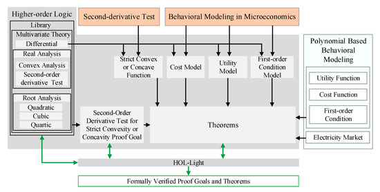
Figure 1.
Proposed methodology for Microeconomics Models in HOL-Light.
- As a first step, we formally model a real strict convex or concave function in higher-order logic. Then, we formally conduct the second-order derivative test to formally determine the strict convexity or concavity of a real function. The results are formally verified using the formal model of the strictly convex function, differential, convex and real analysis theories of HOL-Light.
- In the second step, the above-mentioned formalization is used to formally model the cost and utility functions in higher-order logic. We also formally model the first-order condition for profit maximization problems using differential theory of HOL-Light. These formalizations allow us to formally reason and verify the properties of the given functions within the sound core of HOL-Light theorem prover.
- Finally, we utilize the formalization from Steps 1 and 2 to formally verify the cost, utility, and first-order condition modeling based on the polynomial functions. We use the formalization to formally verify the behavioral modeling employed in the electricity market, for electricity dispatch and DR economic problems.
5. Formalization of Microeconomics Concepts
In this section, we present a higher-order-logic formalization of the second-order derivative test for the strict convexity or concavity of a real function. These formally verified results are further employed to formally model the cost and utility functions in microeconomics. We also present formal modeling of the first-order condition in the HOL-Light theorem prover.
Formalization of Strict-Convexity and Concavity
We formally define a real strict convex function in HOL-Light as:
Definition 2.
Real strict convex function
⊢∀ s f. f real_strict_convex_on s = (∀ x y u v. x ∈ s ∧ y ∈ s ∧ &0 < u ∧ &0 < v ∧ u + v < &1 ⇒ f (u ∗ x + v ∗ y) < u ∗ f x + v ∗ f y).
In the above definition, f:→ represents a real function and s:→ represents a real interval. The above definition differs from Definition 1 by a strict inequality.
Based on Definition 2, we formally verify the scalar multiplication and addition of the two strictly convex functions in HOL-Light, as:
Lemma 1.
constant multiplier property
⊢∀ .
A1: < ∧ A2:
⇒( . ∗
In the above lemma, Assumptions A1–A2 ensure that the constant multiplier is positive and the given function is strictly convex. Under these conditions, the multiplication does not affect the strict convexity of the given function.
Similarly, we formally verify that the addition of the two strict convex functions results in a real strict convex behavior as:
Lemma 2.
Addition property
⊢∀ .
A1: A2:
⇒( . + )
Now, we formally verify the second-order derivative test for the real strict functions, i.e., Equation (3a), in HOL-Light, as:
Theorem 7.
Second-order derivative for real strict convex function
⊢∀ .
A1: ¬(∃. ) ∧
A2: (∀ . ∈⇒( )( ))
A3: (∀ . ∈⇒( )( ))
A4:
⇒()
The above theorem is verified using the mean-value theorem along with the definition of the strict convexity. Assumptions A2–A3 ensure that the function is twice differentiable over the given interval and Assumption A4 ensures that the function is strictly convex. The conclusion of the theorem formally verifies that the second-derivative of the function is positive.
We utilize the strict convexity formalization to formally verify the strict concavity of any given function. It is possible due to the mathematical relationship between two concepts, i.e., the negative of a strictly convex function is strictly concave. The second order derivative test for strict concavity, i.e., Equation (3b), is verified in HOL-Light, as:
Theorem 8.
Second-order derivative for real strict concave function
⊢∀ .
A1: ¬(∃. ) ∧
A2: (∀ . ∈⇒( )( ))
A3: (∀ . ∈⇒( )( ))
A4:
⇒()
Theorem 8 is formally verified by using the definition of the strict convexity and second-order derivative in HOL-Light. In Assumption A4, we utilize the mathematical relationship between the strict convex and strict concave functions, i.e., the negative of a strict convex function is a strict concave function. The conclusion is the formally verified result for the second-order derivative of the given strictly concave function, i.e., second-order derivative of a strictly concave function is negative. We adopted a similar approach for verifying the variants of Lemmas 1 and 2 for strictly concave functions in our formalization.
Now, we formally model the mathematical properties, i.e., continuity, differentiability, monotonicity and convexity or concavity, of the cost and utility functions in HOL-Light. The cost function is modeled in higher-order logic as:
Definition 3.
Convex Cost function
⊢∀ f x.convex_cost_func f s x =
( f real_continuous_on s ) ∧ ( f real_differentiable_on s ) ∧
( ∀ x y. ( x ∈ s ) ∧ ( y ∈ s ) ∧ ( x ≤ y ) ⇒ ( f x ≤ f y ) ) ∧
( f real_convex_on s ) )
Definition 4.
Strictly Convex Cost function
⊢∀ f x. strict_convex_cost_func f s x =
( f real_continuous_on s ) ∧ ( f real_differentiable_on s ) ∧
( ∀ x y. ( x ∈ s ) ∧ ( y ∈ s ) ( x < y ) ⇒ ( f x < f y ) ∧
( f real_strict_convex_on s ) )
Similarly, the utility function is modeled as:
Definition 5.
Concave Utility function
⊢∀ f x. concave_utility_func f s x =
( f real_continuous_on s ) ∧ ( f real_differentiable_on s ) ∧
( ∀ x y. ( x ∈ s ) ∧ ( y ∈ s ) ∧ ( f x ≤ f y ) ) ∧
( -f real_convex_on s )
Definition 6.
Strictly Concave Utility function
⊢∀ f x. strict_concave_utility_func f s x =
( f real_continuous_on s ) ∧ ( f real_differentiable_on s ) ∧
( ∀ x y. ( x ∈ s ) ∧ ( y ∈ s ) ∧ ( f x < f y ) ) ∧
( -f real_strict_convex_on s )
Finally, we formally model the first-order condition, described by Equation (1), in HOL-Light, as:
Definition 7.
First-order Condition
⊢∀ f x. first_order_cond f x = ( real_derivative f x = &0 )
In Definition 7, first_order_cond is a higher-order-logic function, which accepts a real valued function, f, and variable x, whereas real_derivative is a higher-order-logic function representing mathematical derivative of the given real function.
The formalization in this section provides the necessary logical framework to formally verify the cost, utility and first-order condition models within the sound core of the HOL-Light theorem prover.
6. Case Study: Formal Behavioral Modeling Based on Polynomial Functions
Polynomial functions are commonly used in microeconomics models [1,5,42]. We provide formal analysis of the cost and utility modeling based on the polynomial type of functions up to the fourth order. Additionally, we formally verify the first-order condition for the profit functions, which are based on the polynomial type of cost utility functions.
6.1. Polynomial Type of Cost Functions
We formally verify the quadratic cost function as:
Theorem 9.
Quadratic Cost Function
⊢∀ .
A1: ( ) ∧A2:( ) ∧ A3:¬(∃. ) ∧
A4: () ∧
A5: (∈) ∧A6:( < ) A7:( < ) ∧
⇒ < ( ) ∧
< (( ))
In the above theorem, Assumptions A1–A3 represent the conditions on the given interval, i.e., s is a real, open, and non-singular interval. Assumption A4 ensures that the given function satisfies the necessary conditions to model the utility by using Definition 4. Assumption A5 ensures that function is defined over the given interval, whereas Assumptions A6–A7 represent the conditions on the domain of the given function, < , and on the leading coefficient, < , to formally verify the increasing first and second-order derivatives of the quadratic function in the conclusion.
Next, we formally verify the cubic cost function modeling, in the HOL-Light theorem prover, as:
Theorem 10.
Cubic Cost Function
⊢∀ .
A1: ( ) ∧A2:( ) ∧A3:¬(∃. )
A4: ()
A5: (∈) ∧
A6: ( < )) ∧A7:( < ) ∨ ( < )
⇒ < (
))∧
< ((
)))
In the above theorem, Assumptions A6–A7 are conditions on the domain, , of the cubic cost function to formally verify the properties of the increasing first and second-order derivatives in the conclusion.
Theorem 11.
Quartic Cost Function
⊢∀ .
A1: ( ) ∧A2:( ) ∧A3:¬(∃. )
A4: (
)
A5: (∈) ∧ A6:( = ) ∧
A7: ( = ) ∧A8: ( = ) ∧A9: (− = ) ∧
A10: (≤ ∨ ≤ ∨ ≤) ∧
A11: ( < ∨ < )
⇒ < (
)) ∧
< ((
)
In the above theorem, Assumptions A6–A9 provide the relationship between the coefficients of the given quartic polynomial and coefficients of its quadratic factor. Assumptions A10–11 impose conditions on the domain, , of the given polynomial in terms of the coefficients of the linear and quadratic factors of the given quartic cost function, to formally verify the increasing first and second-order derivatives in the conclusion of the theorem.
Theorems 9–11 are formally verified results for the quadratic, cubic and quartic cost functions, mainly, based on Definition 4, Lemma 1, Lemma 2, and Theorem 7, whereas Theorems 2–6 are used to formally specify the domain, of the given polynomials, in which the desired properties of the cost models are satisfied.
6.2. Utility Function
We formally verify the utility functions modeled using the polynomial functions of up to the fourth order, in higher-order logic, as:
Theorem 12.
Quadratic Utility Function
⊢∀ .
A1: ( ) ∧A2:( ) ∧
A3: ¬(∃. ) ∧A4: (∈) ∧
A5: (∀ .( ( ))∧
A6: (≤) ∧ A7: ( < )
⇒ ≤( ) ∧
( (
c ))≤
In the above theorem, Assumption A5 models the necessary conditions for utility modeling by using Definition 5. Assumption A6 ensures that the domain of the given quadratic polynomial, i.e., variable x, is greater than to satisfy the increasing property of utility modeling. Assumption A6 ensures that the leading coefficient is negative, which in turn ascertains the concavity of the given quadratic polynomial. These assumptions ensure the formal verification of the increasing first-order derivate and decreasing second-order derivatives in the conclusion of the theorem.
Theorem 13.
Cubic Utility Function
⊢∀ .
A1: ( ) ∧A2: ( ) ∧
A3: ¬(∃. ) ∧A4:(∈) ∧
A5: (∀ .(
) ∧ A6:(≤) ∨ (≤)
A7: (≤)
⇒(≤( ))
∧ ( (
) ≤)
Assumptions A6 and A7 impose conditions on the real variable, x, which is the domain of the cubic utility function for positive first-order derivative and negative second-order derivative tests.
Next, we formally verify the quartic utility function in higher-order logic as:
Theorem 14.
Quartic Utility Function
⊢∀ .
A1: ( ) ∧A2:( ) ∧ A3:¬(∃. ) ∧
A4: (∈) ∧A5:(∀ .(
))∧A6:( = ) ∧
A7: ( = ) ∧A8:( = ) ∧A9:(− = ) ∧
A10: (≤ ∨ ≤ ∨ ≤) ∧
A11: (≤ ∨ ≤)
⇒( 0 ≤
))∧
( (
))≤
Assumptions A6–A9 relate the coefficients of the linear and quadratic factors of the quartic polynomial coefficients. These conditions formally specify the factorization of the quartic polynomial based on Theorem 3. Assumptions A10 and A11 provide allowable ranges of the domain, x, of the given function to formally verify the positive first-order derivative and negative second-order derivative in the conclusion of the above theorem.
Theorems 12–14 are formally verified using Theorem 1 and Definition 5. Theorem 1 is used to verify the concavity of the polynomial utility functions, whereas, factoring theorems, i.e., Theorems 2–6, are used to formally specify the conditions on the domain of the polynomial type of the utility functions.
6.3. First-Order Condition
Finally, we present formally verified results for the real stationary or critical points for the profit functions designed using polynomial functions. We use Definition 7 to model the first-order condition for the profit function, where is used to model the real function. We use linear revenue function, i.e., = ∗ , in which is the rate of the electricity for the amount of consumed electricity, i.e., . For the cost function, , modeling, we consider quadratic, cubic, and quartic polynomial based behavioral models one by one.
In this regard, profit function based on the quadratic cost or utility function is verified as:
Theorem 15.
First-order condition for quadratic cost function
⊢∀ .
A1: ≠ ∧
A2: =
⇒( ∗ −( ∗ ))
In the above theorem, Assumption A1 ensures that the leading coefficient of the quadratic type of the cost or utility function is not zero. This assumption avoids the possibility of the reduced order case of the polynomial. Assumption A2 specifies the critical point of the given profit function in terms of the rate of electricity, , and coefficients of the given quadratic cost function.
Theorem 15 is formally verified by taking the derivative of the profit function. This allows for formally verifying the above theorem using Assumption A2, which is the critical point of the given function.
Similarly, the profit function based on the cubic type of cost or utility function is formally verified as:
Theorem 16.
First-order condition for cubic cost function
⊢∀ .
A1: ≠ ∧
A2: < − ∗ ∗ ( − ) ∧
< ∧ < ∨
< - ∨
< ∧ < ∨
- <
⇒( ∗ −( )
In the above theorem, Assumption A2 provides the relationship between variable, , and coefficients of the given function to ensure real critical or stationary points.
Finally, we formally verify the first-order condition for profit function, when the cost or utility function is a quartic polynomial, in higher-order logic, as:
Theorem 17.
First-order condition for quartic cost function
⊢∀ .
A1: ≠ ∧A2: = ∧
A3: + ∗ = ∧ A4: + ∗ =
A5: + ∗ = A6: − = ∗
A7: < − ∗ ∗ ∧
< ∧ < ∨
< - ∨
< ∧ < ∨
− <
⇒(
In the above theorem, first-order derivative reduces the given fourth order quartic polynomial to the corresponding third-order polynomial. Assumptions A2–A6 represent the relationship among the coefficients of the cubic ordered profit function and its factors, i.e., linear and quadratic. Assumption A7 gives the relationship between variable x and coefficients for the real stationary points of the profit function.
The proposed foundational formalization of the derivative tests allowed us to formally specify and verify the microeconomics based behavioral modeling of the smart grid entities in DR programs. Theorems 9–17 represent universally quantified results, which unlike traditional techniques, also contain exact and exhaustive set of the assumptions to model the behavior of the given entities. These results give very useful insights about the behavior of the modeling function, with respect to its domain, to satisfy the desired mathematical properties. For example, the assumptions in Theorems 9–14 provide explicit conditions on the domain of the commonly used polynomial type of the cost and utility functions in DR programs [42,43,44,45,46,47]. Similarly, the assumptions of Theorems 15–17 provide a priori information regarding the effect of the values of the coefficients of the given profit function on the maximum possible profit. In the case of real profit function, the assumptions of Theorem 15–17 facilitate choosing the values of the coefficients of the profit function for the real maximum of the given profit function.
The proposed formalization is generic and can be readily employed to formally verify and specify any microeconomics model based on the different mathematical functions, such as exponential and logarithmic. The main challenges faced in the proposed formalization were to provide formally verified theorems related to strict convexity or concavity and associated properties of such functions to enable the formalization of the microeconomics concepts. Besides the development of the fundamental logical framework, the formal verification of the case study involved considerable effort due to the rigorous formal reasoning required to accomplish the task using theorem proving. The corresponding proof script, which is available for download at [48], has 2000 lines of HOL-Light code and required about 250 man hours of development time.
7. Electricity Market Applications
In this section, we formally verify the quadratic cost [49] and utility [44] models, which have been used in the optimal power flow [50] and DR programs [44] in the electricity market. In optimal power flow, polynomial functions are used to find the economic dispatch, which ensures reduced electricity generation cost, whereas DR programs are used to change the demand behavior of the consumers to ensure the safe and secure smart grid operations. In this regard, incentive and time based programs are employed to change the electricity usage behavior of the smart grids.
7.1. Quartic Polynomial Cost Function for Thermal Power Plants
We formally verify the quadratic polynomial cost function for thermal power plants using the results of Section 6. A metahuristic algorithm in [49], called the ABC algorithm, has been utilized for estimating the coefficients of the quadratic type of the cost function for the economic dispatch problem, which is used in the operation economics to reduce the cost of electricity generation. In the economic dispatch problem, distributed generators are used to produce electricity to reduce the total operational cost and regulation issues in an electricity market. The mathematical form for the quartic cost function is:
where , , , , , and represent the cost function for electricity generation, amount of the power generated, coefficients, and error associated with the j-th generator. Equation (4) is used to estimate the parameters for three different thermal power plants with fuels such as coal, oil, and gas [49]. Each power plant consists of five generating units with 10, 20, 30, 40, and 50 MW. The estimation is performed on the actual data [51] and presented in Table 2.
Table 2.
Estimated coefficients of cubic cost function using the ABC algorithm.
We formally verify the mathematical properties of the cost function, in HOL-Light, as:
Theorem 18.
Quadratic Cost Function for Economic Dispatch
⊢∀ .
A1: (∈)
⇒ < ( ) ∧
< ((
) ∧
< ( ) ∧
< ((
) ∧
< ( ) ∧
< (
)
In the above theorem, the quadratic cost function for coal, oil, and gas power plants is formally verified using Theorem 9. Thanks to our foundational formalization, the proof of Theorem 18 just required a few lines of HOL-Light code. The formally verified results ensure that all the mathematical properties, in Definition 4, for modeling the cost function are satisfied by the estimated quadratic polynomial cost functions.
7.2. Quadratic Utility Function for Smart Grids
We formally verify a quadratic utility function, using our proposed formalization in Section 6, which is used in [44] to find the optimal energy consumption levels for the smart grid users. The proposed algorithm in [44] relies on the real-time pricing for DR management by exploiting the utility maximization concept of microeconomics. The algorithm considers a smart grid environment that is equipped with smart meters and communication network for interacting among energy provider and end-users in the smart grid network. The quadratic utility function is defined as [44]:
The function represents utility function for different users in the smart grid network, where varies among the electricity users in the network to differentiate users, such as industrial or household, and is a predetermined parameter. The utility for a particular consumer is a function of its electricity consumption, i.e., x.
Furthermore, the utility function is also employed to design the welfare objective function, , of an individual consumer, as:
where P is the price of the x(MW) amount of the electricity consumption of a user. The welfare objective function is maximized using the first-order condition,
We formally verify the behavior of the quadratic utility function, i.e., Equation (5), and utility maximization problem, i.e., Equation (6), for and for a single consumer in interval, as:
Theorem 19.
Quadratic utility function for the real-time algorithm
⊢∀ .
A1: (∈)
⇒≤( )∧
(( ≤)
The above theorem is formally verified using Theorem 12. Assumption A1 ensures that the electricity demand of an individual consumer is within the allowed consumption levels. Moreover, assumptions of Theorem 12 are also verified to accomplish the verification of the given utility function.
Similarly, the first-order condition for the welfare objective is formally verified as:
Theorem 20.
First-order condition for Welfare objective function
⊢∀ .
A1: ( = ∗ −)
⇒(( ∗ −( ))=)
The above theorem is formally verified using Theorem 15. Assumption A1 is the necessary condition for the profit maximization of the welfare function in terms of the electricity price, P, and maximum electricity consumption level. Again, the proof of Theorems 19 and 20 just required a few lines of HOL-Light code, which illustrates the usefulness and practical effectiveness of the proposed formalization of foundational theories. Theorem 19 ensures that utility function satisfies the mathematical properties of Definition 6, whereas Theorem 20 gives explicit conditions for the maximization of the welfare function.
8. Conclusions
In this paper, we presented a formal methodology to conduct the formal behavioral modeling and analysis of microeconomics concepts. The derivative tests are primary mathematical techniques to specify and verify the desired properties, such as monotonicity and convexity, of the modeling functions in microeconomics. To formally model the microeconomics concepts, we formally verified second-order derivative tests for strict convexity or concavity, and, based on these results, we provided the formal models of the cost and utility functions. Additionally, we also developed the formal modeling of the first order condition, which is based on the first-order derivative, to formally analyze the profit functions for profit maximization problems. As a case study, the formalization is employed for the formal behavioral modeling and analysis of the cost and utility modeling based on the polynomial function. Finally, the quadratic cost and utility functions for the economic dispatch problem and DR program are formally verified using the proposed formalization. The distinguishing features of the proposed analysis work include its accurate results due to the involvement of sound theorem proving and the availability of an exhaustive set of assumptions that are required for the validity of the results.
The proposed formalization can be readily employed to formally specify and verify the microeconomics models, such as exponential and logarithmic functions, for any underlying market agent. Moreover, the formalization is based upon the second-order derivative tests, which are abundantly used in the convex theory. Thus, the formalization is also beneficial for a wide range applications of the convex theory [52,53]. The reported formalization supports real analysis with single variable only and thus can be extended to multivariate analysis, which is supported by HOL-Light theorem prover. Moreover, linking conventional analysis tools, such as Maxima [17], with a theorem prover, such as HOL-Light, is also an interesting direction for facilitating formal non-experts to conduct highly reliable and accurate microeconomics analysis of economy markets, using the proposed formalization.
Author Contributions
Conceptualization, F.A. and N.B.; Formal analysis, A.A. and O.H.; Methodology, A.A. and O.H.; Writing—original draft, A.A.; Writing—review and editing, A.A., O.H., F.A. and N.B. All authors have read and agree to the published version of the manuscript.
Funding
This work is supported by ICT Fund UAE, fund No. 21N206 at UAE University, Al Ain, United Arab Emirates.
Conflicts of Interest
The authors declare no conflicts of interest.
References
- Mas-Colell, A.; Whinston, M.D.; Green, J.R. Microeconomic Theory; Oxford University Press: New York, NY, USA, 1995; Volume 1. [Google Scholar]
- Wilkinson, N.; Klaes, M. An Introduction to Behavioral Economics Third Edition; Macmillan International Higher Education: London, UK, 2017. [Google Scholar]
- Coleman, J.S.; Fararo, T.J. Rational Choice Theory; Sage: New York, NY, USA, 1992. [Google Scholar]
- Levin, J.; Milgrom, P. Introduction to Choice Theory. 2004, Volume 20202. Available online: https://web.stanford.edu/~jdlevin/Econ%20202/Choice%20Theory.pdf (accessed on 18 January 2020).
- Henderson, J.M.; Quandt, R.E. Microeconomic Theory: A mathematical Approach; McGraw-Hill: New York, NY, USA, 1971. [Google Scholar]
- Gan, D.; Feng, D.; Xie, J. Electricity Markets and Power System Economics; CRC Press: Boca Raton, FL, USA, 2013. [Google Scholar]
- Hasanpor Divshali, P.; Choi, B.J. Electrical market management considering power system constraints in smart distribution grids. Energies 2016, 9, 405. [Google Scholar] [CrossRef]
- Nafi, N.S.; Ahmed, K.; Gregory, M.A.; Datta, M. A survey of smart grid architectures, applications, benefits and standardization. J. Netw. Comput. Appl. 2016, 76, 23–36. [Google Scholar] [CrossRef]
- Srinivasan, S. Power relationships: Marginal cost pricing of electricity and social sustainability of renewable energy projects. Technol. Econ. Smart Grids Sustain. Energy 2019, 4, 13. [Google Scholar] [CrossRef]
- Arefin, S.S.; Das, N. Optimized hybrid wind-diesel energy system with feasibility analysis. Technol. Econ. Smart Grids Sustain. Energy 2017, 2, 9. [Google Scholar] [CrossRef]
- Siddiqui, A.N.; Thomas, M.S. Techno-economic evaluation of regulation service from SEVs in smart MG system. Technol. Econ. Smart Grids Sustain. Energy 2016, 1, 15. [Google Scholar] [CrossRef]
- Strielkowski, W. Social and economic implications for the smart grids of the future. Econ. Sociol. 2017, 10, 310. [Google Scholar] [CrossRef]
- Ketter, W.; Collins, J.; Block, C.A. Smart Grid Economics: Policy Guidance through Competitive Simulation; Erasmus Research Institute of Management (ERIM): Rotterdam, The Netherlands, 2010. [Google Scholar]
- Moretti, M.; Djomo, S.N.; Azadi, H.; May, K.; De Vos, K.; Van Passel, S.; Witters, N. A systematic review of environmental and economic impacts of smart grids. Renew. Sustain. Energy Rev. 2017, 68, 888–898. [Google Scholar] [CrossRef]
- Greer, M. Electricity Cost Modeling Calculations; Academic Press: Cambridge, MA, USA, 2010. [Google Scholar]
- Deng, R.; Yang, Z.; Chow, M.Y.; Chen, J. A survey on demand response in smart grids: Mathematical models and approaches. IEEE Trans. Ind. Inform. 2015, 11, 570–582. [Google Scholar] [CrossRef]
- Maxima. 2019. Available online: http://maxima.sourceforge.net/l (accessed on 15 December 2019).
- Wolfram Mathematica. 2019. Available online: https://www.wolfram.com/mathematica/analysis/content/ComputerAlgebraSystems.html (accessed on 15 December 2019).
- Wetzstein, M.E. Microeconomic Theory Second Edition: Concepts and Connections; Routledge: New York, NY, USA, 2013. [Google Scholar]
- Stoutemyer, D.R. Crimes and misdemeanors in the computer algebra trade. Not. Am. Math. Soc. 1991, 38, 778–785. [Google Scholar]
- Woodcock, J.; Larsen, P.G.; Bicarregui, J.; Fitzgerald, J. Formal methods: Practice and experience. ACM Comput. Surv. (CSUR) 2009, 41, 19. [Google Scholar] [CrossRef]
- Clarke, E.M.; Grumberg, O.; Long, D.E. Model checking and abstraction. ACM Trans. Program. Lang. Syst. (TOPLAS) 1994, 16, 1512–1542. [Google Scholar] [CrossRef]
- Harrison, J.; Urban, J.; Wiedijk, F. History of Interactive Theorem Proving. In Computational Logic; North Holland: Oxford, UK, 2014; Volume 9, pp. 135–214. [Google Scholar]
- Hackenberg, G.; Irlbeck, M.; Koutsoumpas, V.; Bytschkow, D. Applying formal software engineering techniques to smart grids. In Proceedings of the First International Workshop on Software Engineering Challenges for the Smart Grid, Zurich, Switzerland, 3 June 2012; pp. 50–56. [Google Scholar]
- Mahmood, A.; Hasan, O.; Gillani, H.R.; Saleem, Y.; Hasan, S.R. Formal reliability analysis of protective systems in smart grids. In Proceedings of the 2016 IEEE Region 10 Symposium (TENSYMP), Bali, Indonesia, 9–11 May 2016; pp. 198–202. [Google Scholar]
- Akram, W.; Niazi, M.A. A formal specification framework for smart grid components. Complex Adapt. Syst. Model. 2018, 6, 5. [Google Scholar] [CrossRef]
- Patil, S.; Zhabelova, G.; Vyatkin, V.; McMillin, B. Towards formal verification of smart grid distributed intelligence: Freedm case. In Proceedings of the IECON 2015—41st Annual Conference of the IEEE Industrial Electronics Society, Yokohama, Japan, 9–12 November 2015; pp. 003974–003979. [Google Scholar]
- Gupta, P.K.; Schaetz, B. Constraint-based graceful degradation in smart grids. In Proceedings of the 2nd International Workshop on Software Engineering for Smart Cyber-Physical Systems, Austin, TX, USA, 16 May 2016; pp. 8–14. [Google Scholar]
- Vahebi, M.; Iran, G.; Sadeghzadeh, M.; Atani, R.E. Modeling and Analysis of Reliability in Grid using Petri Nets. Int. J. Comput. Appl. Technol. Res. 2013, 2, 726–730. [Google Scholar] [CrossRef]
- Mhadhbi, Z.; Zairi, S.; Gueguen, C.; Zouari, B. Validation of a distributed energy management approach for smart grid based on a generic colored Petri nets model. J. Clean Energy Technol. 2018, 6, 20–25. [Google Scholar] [CrossRef]
- Calderaro, V.; Hadjicostis, C.N.; Piccolo, A.; Siano, P. Failure identification in smart grids based on petri net modeling. IEEE Trans. Ind. Electron. 2011, 58, 4613–4623. [Google Scholar] [CrossRef]
- Zeineb, M.; Sajeh, Z.; Belhassen, Z. Generic colored petri nets modeling approach for performance analysis of smart grid system. In Proceedings of the 2016 7th International Renewable Energy Congress (IREC), Hammamet, Tunisia, 22–24 March 2016; pp. 1–6. [Google Scholar]
- Dey, A.; Chaki, N.; Sanyal, S. Modeling smart grid using generalized stochastic petri net. arXiv 2011, arXiv:1108.4139. [Google Scholar]
- Chen, T.M.; Sanchez-Aarnoutse, J.C.; Buford, J. Petri net modeling of cyber-physical attacks on smart grid. IEEE Trans. Smart Grid 2011, 2, 741–749. [Google Scholar] [CrossRef]
- HOL-Light Theorem Prover. 2019. Available online: https://www.cl.cam.ac.uk/~jrh13/hol-light/ (accessed on 15 December 2019).
- HOL Theorem Prover. 2019. Available online: https://hol-theorem-prover.org/ (accessed on 15 December 2019).
- Isabelle/HOL Theorem Prover. 2019. Available online: https://isabelle.in.tum.de/ (accessed on 15 December 2019).
- Ahmed, A.; Hasan, O.; Awwad, F. Formal Stability Analysis of Control Systems. In International Workshop on Formal Techniques for Safety-Critical Systems; Springer: Heidelberg, Germany, 2018; pp. 3–17. [Google Scholar]
- Zill, D.; Wright, W.S.; Cullen, M.R. Advanced Engineering Mathematics; Jones & Bartlett Learning: Burlington, VT, USA, 2011. [Google Scholar]
- Hales, T.; Adams, M.; Bauer, G.; Dang, T.D.; Harrison, J.; Le Truong, H.; Kaliszyk, C.; Magron, V.; McLaughlin, S.; Nguyen, T.T.; et al. A Formal Proof of the Kepler Conjecture; Forum of Mathematics, Pi; Cambridge University Press: Cambridge, UK, 2017; Volume 5. [Google Scholar]
- Harrison, J. Floating point verification in HOL light: the exponential function. In Proceedings of the International Conference on Algebraic Methodology and Software Technology, Sydney, NSW, Australia, 13–17 December 1997; Springer: Berlin/Heidelberg, Germany, 1997; pp. 246–260. [Google Scholar]
- Debertin, D.L. Applied Microeconomics: Consumption, Production and Markets; CreateSpace Independent Publishing Platform: Scotts Valley, CA, USA, 2012. [Google Scholar]
- Bessembinder, H.; Lemmon, M.L. Equilibrium pricing and optimal hedging in electricity forward markets. J. Financ. 2002, 57, 1347–1382. [Google Scholar] [CrossRef]
- Samadi, P.; Mohsenian-Rad, A.H.; Schober, R.; Wong, V.W.; Jatskevich, J. Optimal real-time pricing algorithm based on utility maximization for smart grid. In Proceedings of the 2010 First IEEE International Conference on Smart Grid Communications, Gaithersburg, MD, USA, 4–6 October 2010; pp. 415–420. [Google Scholar]
- Wang, Q.; Liu, X.; Du, J.; Kong, F. Smart charging for electric vehicles: A survey from the algorithmic perspective. IEEE Commun. Surv. Tutor. 2016, 18, 1500–1517. [Google Scholar] [CrossRef]
- Wolak, F.A. Identification and Estimation of Cost Functions Using Observed Bid Data: An Application to Electricity Markets; National Bureau of Economic Research: Cambridge, MA, USA, 2001. [Google Scholar]
- Fahrioglu, M.; Alvarado, F.L. Using utility information to calibrate customer demand management behavior models. IEEE Trans. Power Syst. 2001, 16, 317–322. [Google Scholar] [CrossRef]
- Ahmed, A. Formal Beahvioral Modeling in Microeconmics Models. Available online: http://save.seecs.nust.edu.pk/projects/fcumm/ (accessed on 16 December 2019).
- Sönmez, Y. Estimation of fuel cost curve parameters for thermal power plants using the ABC algorithm. Turk. J. Electr. Eng. Comput. Sci. 2013, 21, 1827–1841. [Google Scholar] [CrossRef]
- Qiu, Z.; Deconinck, G.; Belmans, R. A literature survey of optimal power flow problems in the electricity market context. In Proceedings of the 2009 IEEE/PES Power Systems Conference and Exposition, Seattle, WA, USA, 15–18 March 2009; pp. 1–6. [Google Scholar]
- El-Hawary, M.; Mansour, S. Performance evaluation of parameter estimation algorithms for economic operation of power systems. IEEE Trans. Power Appar. Syst. 1982, 574–582. [Google Scholar] [CrossRef]
- Liu, X.; Lu, P.; Pan, B. Survey of convex optimization for aerospace applications. Astrodynamics 2017, 1, 23–40. [Google Scholar] [CrossRef]
- Niculescu, C.; Persson, L.E. Convex Functions and Their Applications; Springer: Heidelberg, Germany, 2006. [Google Scholar]

© 2020 by the authors. Licensee MDPI, Basel, Switzerland. This article is an open access article distributed under the terms and conditions of the Creative Commons Attribution (CC BY) license (http://creativecommons.org/licenses/by/4.0/).