All articles published by MDPI are made immediately available worldwide under an open access license. No special
permission is required to reuse all or part of the article published by MDPI, including figures and tables. For
articles published under an open access Creative Common CC BY license, any part of the article may be reused without
permission provided that the original article is clearly cited. For more information, please refer to
https://www.mdpi.com/openaccess.
Feature papers represent the most advanced research with significant potential for high impact in the field. A Feature
Paper should be a substantial original Article that involves several techniques or approaches, provides an outlook for
future research directions and describes possible research applications.
Feature papers are submitted upon individual invitation or recommendation by the scientific editors and must receive
positive feedback from the reviewers.
Editor’s Choice articles are based on recommendations by the scientific editors of MDPI journals from around the world.
Editors select a small number of articles recently published in the journal that they believe will be particularly
interesting to readers, or important in the respective research area. The aim is to provide a snapshot of some of the
most exciting work published in the various research areas of the journal.
This paper proposes an effective method for determining thermal stresses in structural elements with a three-dimensional transient temperature field. This is the situation in the case of pressure elements of complex shapes. When the thermal stresses are determined by the finite element method (FEM), the temperature of the fluid and the heat transfer coefficient on the internal surface must be known. Both values are very difficult to determine under industrial conditions. In this paper, an inverse space marching method was proposed for the determination of the heat transfer coefficient on the active surface of the thick-walled plate. The temperature and heat flux on the exposed surface were obtained by measuring the unsteady temperature in a small region on the insulated external surface of a pressure component that is easily accessible. Three different procedures for the determination of the heat transfer coefficient on the water-spray surface were presented, with the division of the plate into three or four finite volumes in the normal direction to the plate surface. Calculation and experimental tests were carried out in order to validate the method. The results of the measurements and calculations agreed very well. The computer calculation time is short, so the technique can be used for online stress determination. The proposed method can be applied to monitor thermal stresses in the components of the power unit in thermal power plants, both conventional and nuclear.
In modern energy systems, wind farms have a significant share in the production of electricity, which is characterized by the high variability of the generated power over time. Thermal power plants must, therefore, be adapted to fast start-ups, shutdowns, and rapid load changes. Cyclical operation of the power unit as well as start-ups and shutdowns cause high thermal stresses in thick-walled pressure elements, which can significantly reduce the service life of these elements [1,2,3]. The thermal stresses are very much influenced by the heat transfer coefficient on the surface where the heat transfer takes place. Due to the severe difficulties in determining the actual heat transfer coefficient, especially under transient conditions, simplifying assumptions are made, which, however, reduce the accuracy of the calculations of the stresses. In [4], emergency cooling of the double-layered nuclear reactor pressure vessel was modeled. Due to the large ratio of the reactor diameter to the wall thickness, which was larger than ten, computer modeling as well as experimental studies were carried out on the double-layered plate. The plate was heated to a high initial temperature and then the cladding was sprayed with cold water at the temperature of 20 °C. In the computer simulation, it was assumed that the sprayed surface of the cladding immediately takes the temperature of the cooling water, which was 20 °C. The thermal stresses calculated in this way were overestimated. Raafat et al. [5] calculated the thermal stresses and fatigue wear of a submerged steel pipeline. The temperature of the inner pipe surface was assumed to be equal to the maximum design temperature of the fluid, which was 50 °C. Such an assumption means that an infinite large heat transfer coefficient at the pipe inner surface was adopted. In the study by Guo et al. [6], thermal and stress analysis in a novel dual pipeline system was carried out. The temperature of the supercritical steam flowing inside the central pipeline was 700 °C. To reduce the temperature of the primary steel pipe, its inner surface was coated with a protective layer made of low-conductivity ceramics. When calculating the temperature field in a dual-pipe system, the temperature of the internal surface of the thermal barrier coating (TBC) was assumed to be equal to the temperature of the supercritical steam. The convective thermal resistance was then neglected, adopting an infinite large heat transfer coefficient.
Local and mean heat transfer coefficients can be measured using the naphthalene sublimation technique [7] or utilizing color change coatings [8]. Gultekin and Gore [9] demonstrated that nuclear magnetic resonance can be used for the measurement of low-value heat transfer coefficients. However, the three measurement techniques presented in [7,8,9] can be applied in the laboratory, when the fluid temperature is much lower than the fluid temperature in the high-pressure components of power plants.
For the experimental estimation of the heat transfer coefficient, the solution of the inverse heat conduction problem can be used. After calculating the temperature and heat flux on the surface of the solid using the solution of the inverse heat conduction problem and knowing the temperature of the fluid from the measurement, the heat transfer coefficient can be determined. An example of such a method of determining the heat transfer coefficient is presented, among others, in [10]. The method of the least squares was used to solve the inverse heat conduction problem. At first, the time derivative in the heat conduction equation was replaced by the backward finite difference quotient. The resulting ordinary differential equation was then solved by an approximate analytical method with the Chebyshev polynomials of the k-th degree as base functions. However, most of the mathematical procedures for solving inverse heat conduction problems are so complicated that they are only suitable for determining the heat transfer coefficient off-line due to the large amount of time required for computer calculations. For the online determination of the heat transfer coefficient, the method of solving the inverse problem should be simple, so that the computer calculation time is very short.
Zhu et al. [11] conducted an experimental strength analysis of the aluminum tank during its cooling while filling it with liquid nitrogen. The cylindrical wall of the tank was treated as a flat wall. This assumption was fully justified as the ratio of tank diameter D to its thickness s was greater than 10. When D/s > 10, the cylindrical wall can be treated as flat, according to the material mechanics manual [12]. The thermal stresses were determined by measuring the strains on the outer surface of the container in axial and circumferential directions.
To identify thermal stresses in pressure elements in transient states, the fluid temperature [13,14,15,16] and the heat transfer coefficient at the surface in contact with the fluid must be known. The heat transfer coefficient is determined by the temperature of the high-pressure fluid and the temperature of the surface in contact with the fluid. Since the differences between them are small, very accurate measurements of the transient temperature of the fluid are necessary. The heat transfer coefficient value has a considerable influence on the optimum rate of fluid temperature change, which is determined by the condition that the stress limit values on the internal surface of the pressure element must not be exceeded [17].
It is difficult to carry out temperature measurements on the internal surface of a pressure element, particularly when the values of pressure, temperature, and velocity of the fluid are high. Temperature sensors cannot always be mounted on the surface of the pressure element and, furthermore, contact resistance can cause the measured temperature to be disturbed by significant errors. For a one-dimensional field of transient temperature, the heat transfer coefficient of the internal pipe surface can be determined by measuring the wall temperature near the inner pipe surface [18]. In nuclear power plants, it is not permitted to drill holes in the walls of pressure elements. In such cases, the coefficient of heat transfer on the internal surface is determined based on the temperature measured on the insulated, easily accessible external surface of the element [19]. If the temperature field is three-dimensional, as is usually the case with pressure elements with complex geometry, then to determine the temperature and heat flux on the internal surface, it is necessary to measure the temperature at several ten points on the external surface. This approach can also be used in conventional power plants, as the thermocouples are mounted on an easily accessible external surface. The paper presents the online method of determining the transient coefficient of heat transfer on the internal surface of the element based on the measurement of the temperature of the external surface. The measurement technique proposed in [13,14,15,16] can be used to determine the unsteady temperature of the fluid with high accuracy. By knowing the heat transfer coefficient and fluid temperature, which are determined online, the thermal stresses can also be calculated online. Commercial programs based on the FEM can be used to calculate thermal stresses, taking into account the real-time variations of the fluid temperature and heat transfer coefficient. The proposed thermal stress monitoring method can be used to control thermal stresses in critical pressure elements such as drums in conventional power plants or reactor pressure vessels in nuclear power plants.
2. Method for the Determination of the Transient Three-Dimensional Temperature Distribution in the Plate and the Heat Transfer Coefficient on its Exposed Surface
The experimental stand allows the identification of the transient heat transfer coefficient on the vertical surface of the water-sprayed plate. A thick-walled plate was selected for the test because of the more comfortable control of the experimental conditions such as the arrangement of thermocouples on the heated surface of the plate, the control of the positions of the thermocouple joints inside the plate, or the measurement of the exposed surface temperature of the plate using a thermal imaging camera.
A thick-walled plate brings the cylindrical wall well closer when the ratio of the average diameter of the cylindrical element to the wall thickness is higher than 10 [12]. Such conditions are met by the conventional boiler drums and pressure vessels of nuclear reactors, where the ratio of diameter to wall thickness is between 15 and 20. Following the same procedure as for the plate under test, appropriate equations for a cylindrical or spherical wall can also be derived, if necessary.
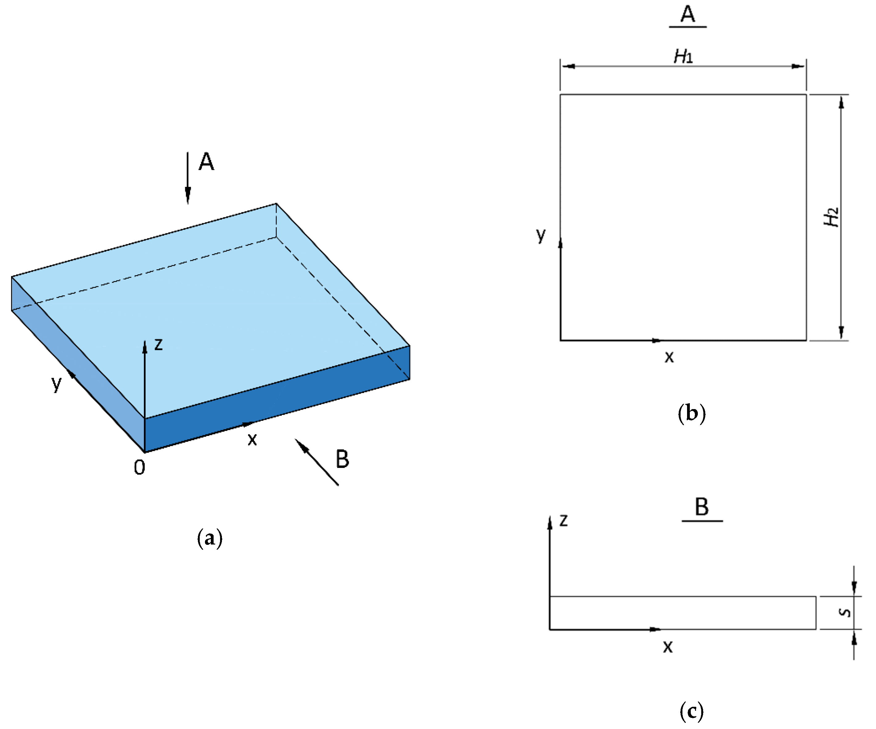
In the analyzed case, it was assumed that heat was transferred in all three directions: x, y, and z. The temperature distribution inside the slab (Figure 1) was determined using the inverse marching method. In Figure 1, the height, width, and thickness of the slab are indicated by the symbols H1, H2, and s, respectively.
The transient heat conduction equation is written in the Cartesian coordinate system (x,y,z) and is given by [20]:
where c, ρ, k are the specific heat, density, and heat transfer coefficient, respectively; T is the temperature; and t denotes the time. Based on the temperature Tout measured on one surface of the slab (for z = 0):
where the temperature distribution over the thickness of the slab was determined including its second surface (for 0 < z ≤ s).
The presented calculation method assumed that one of the surfaces (for z = 0), on which temperature measurements were carried out, was thermally insulated. The second boundary condition results from this assumption:
In summary, for the surface z = 0, two boundary conditions were formulated, as defined by Equations (2) and (3), while the boundary condition for the surface z = s was to be determined. The lateral surfaces of the slab were thermally insulated, so their perfect insulation can be assumed:
The problem formulated by Equations (1)–(4) is an inverse problem, the solution of which was obtained by the finite volume method. The division of the slab into three layers of control volumes is shown in Figure 2a and into four layers of control volumes in Figure 2b. Three or four control volumes (nodes) on the thickness of the plate are sufficient to solve the inverse problem with satisfactory accuracy [21,22]. Contrary to direct heat conduction problems, which are well-conditioned, increasing the number of control volumes on the plate thickness over four does not lead to increasing the accuracy of the inverse solution. The influence of the number of control volumes on the temperature and heat flux on the exposed plate surface is discussed in detail in [21].
For all nodes located in the control volumes centers, the finite volume method can be used to write the energy balance equations.
The energy conservation equation for the node with coordinates (xi, yj, zk) inside the analyzed control volume is:
The energy conservation in Equation (5) has been written for all nodes Pi, j, k = P(xi, yj, zk) that are situated at the centers of gravity of finite volumes, as shown in Figure 3 and Figure 4. The coordinates of nodes P(xi, yj, zk) at the center of the finite volumes are specified, as shown below:
To solve the inverse problem, the analyzed thick-walled plate is divided into finite volumes (Figure 2, Figure 3 and Figure 4). First, the case where the plate is divided into three control volumes in the z-axis direction was considered. The solution of the inverse problem was started by writing the equations of energy balance for 25 nodes lying on the insulated surface of the slab z = 0 (Figure 3a,d). Then, from these equations, the time-dependent temperatures in 13 nodes lying in the plane z = Δz (Figure 3b,d) are determined. Similarly, from the energy balance equations written for 13 nodes in the plane z = Δz, the temperatures at five points in the plane z = 2Δz (Figure 3c,d), in direct contact with the fluid, are determined.
The finite volumes, in the middle of which the temperature is measured or determined, lying in different planes z are marked with different colors (Figure 2, Figure 3 and Figure 4). With the use of the computational algorithm described above, the temperature at points (4,5,3), (3,4,3), (4,4,3), (5,4,3), and (4,3,3) is found. To determine the heat transfer coefficient at node (4,4,3) (Figure 3c,d), located on the cooled plate surface, the normal component of the heat flux at the same point has been calculated as follows:
(1)
Approximating the temperature derivative with a differential quotient with the first-order of accuracy (Method I) [17]
(2)
Approximating the temperature derivative with a differential quotient with the second-order of accuracy (Method II) [17]
(3)
From the energy conservation equation for the node (4,4,3) assuming three-dimensional heat conduction (Method III)
The heat transfer coefficient h on the exposed surface z = 2Δz = s is defined as follows:
A novel thermometer was designed to measure the temperature of a fluid with high accuracy at high temperature and pressure [13,14,15]. An appropriate calculation procedure was also developed [13,14,15]. The proposed measuring technique reduces the dynamic errors in fluid temperature measurements, which are very large under industrial conditions if conventional thermometers are used.
The above procedure for determining the heat transfer coefficient on the exposed surface relates to the division of the thickness of the plate into three control volumes. An analogous analysis was performed for a more dense division of the plate into control volumes when there were four control volumes on the plate thickness (Figure 4).
To determine the temperature, at one point on the exposed surface, it is necessary to measure the temperature at 15 points on the opposite surface of the plate with its division into three finite volumes or 25 points with its division into four finite volumes. The temperature of the cooling water was measured. Due to the large mass flow rate of cooling water and the vertical position of the heated plate, the temperature increase of water on the plate was small. Therefore, the temperature of water in Equation (10) was assumed to be the temperature of water at the outlet from nozzles equal to 16 °C. The calculated plate temperatures at selected points were compared with the measured temperatures.
3. Verification of the Method by Experimental Tests
The test rig (Figure 5) was used for the experimental verification of the proposed inverse procedure for the determination of the temperature distribution and heat transfer coefficient at the exposed surface of a thick-walled slab. The slab was made of St3S steel with the following dimensions: H1 = 0.8 m, H2 = 0.8 m, and s = 0.035 m.
One face of the plate, 1 (the outer surface), was heated by the silicone heater, 2. The maximum power of the 600 mm × 600 mm and 2 mm thick heater was 2500 W. Resistance wires were evenly distributed in the silicone heater, with a pitch of about 5 mm. The power of the heater could be changed continuously. To prevent heat loss, the heating panel was thermally insulated with mineral wool. The front surface of the plate, 1, was spray cooled by nine nozzles, 5, located in nine openings, 7, in the top plate, 6. Nozzles were supplied with water from a distributor, 8, with nine stubs, 9, connected by flexible hoses with nozzles.
The temperature was measured at 42 points located on the heated surface. One thermocouple was located on an exposed chilled surface. The locations of the thermocouples coincided with the locations of the nodes in the control volume grid (Figure 3a). The control volume dimensions in the x-axis and y-axis direction were Δx = 0.085 m and Δy = 0.085 m, respectively. The control volume height in the z-axis direction was Δz = 0.0175 m for the division of the plate thickness into three control volumes and Δz = 0.0117 m for the division of the plate thickness into four control volumes.
The experimental stand allows for the identification of the transient heat transfer coefficient on the vertical surface of the water-sprayed plate. A thick-walled plate was selected for the test because of the easier control of the experimental conditions such as the arrangement of thermocouples on the heated surface of the plate, the control of the positions of the thermocouple joints inside the plate, or the measurement of the exposed surface temperature of the plate using a thermal imaging camera.
A thick-walled panel brings the cylindrical wall well closer when the ratio of the average diameter of the cylindrical element to the wall thickness is greater than 10 [12]. Such conditions are met by the conventional boiler drums and pressure vessels of nuclear reactors where the ratio of diameter to wall thickness is between 15 and 20. Following the same procedure as for the plate under test, appropriate equations for a cylindrical or spherical wall can also be derived, if necessary.
Before spraying with water, the plate was heated to approximately 70 °C and then cooled. This temperature was chosen for safety reasons during the experiment. However, it should be emphasized that the proposed method of determining the heat transfer coefficient will also work well at much higher pressure as well as at a higher temperature of the pressure element. For example, under ultra-supercritical conditions, the steam pressure can be higher than 30 MPa and the steam temperature is about 700 °C. The method is also effective at such high steam parameters because the thermocouples are attached to the external, easily accessible surface of the pressure element.
A thick-walled water-sprayed plate was selected as the construction element under test. Similar operating conditions such as during water spraying of the plate occur during the emergency cooling of a nuclear reactor pressure vessel and in conventional thermal power plants. When the steam condensate flowing in the lower part of a horizontal pipeline hits the opposite wall of the pipeline elbow at a much higher temperature than the condensate temperature, a shock cooling of the elbow occurs.
The inverse heat conduction problem was solved to determine the unsteady temperature distribution in the slab. By using the measured temperature histories at the nodes situated on the heated insulated surface, the temperature values on the sprayed surface and inside the slab wall at distances z = Δz and z = 2Δz from the heated surface were calculated for the division of the plate thickness into three control volumes. When dividing the plate thickness into four control volumes, the temperature of the plate was determined in nodes situated in planes with the coordinates: z = Δz, z = 2Δz, and z = 3Δz. The following thermal properties of the mild steel St3S, from which the plate was made, were adopted in the inverse analysis: ρ = 7850 kg/m3, c = 460 J/(kg·K), and k = 58 W/(m·K). The time step was Δt = 4 s. To reduce the influence of random errors that the measured temperature variations are burdened with, a 9-point moving digital filter was used to smooth measured temperatures [17].
A characteristic feature of all methods for solving inverse heat conduction problems is their high sensitivity to random temperature measurement errors. This is due to the high damping and delay of temperature changes occurring at points inside the solid compared to changes at the active surface. In the case of the inverse problem, if at a given internal point, the measured temperature at the next point in time suddenly changes due to a random measurement error, then to achieve such a difference, the change in temperature or heat flux on the active surface must be much greater.
To ensure greater stability of the results of the inverse solution, it is best to remove random measurement errors from the measured temperatures, which are the input to the inverse solution. One of the more useful tools for stabilizing the inverse solution is to smooth the measured temporal temperature changes using the digital filters proposed in [17].
4. Results and Discussion
The inverse problem of heat conduction in the plate is solved by dividing the plate into three and four control volumes in the z-axis direction. The coefficient of heat transfer on the active surface was determined using three different formulas. In the first formula, the heat flux was calculated using a finite-difference of the first-order accuracy, using temperatures in the node located at the active surface and the adjacent node in the normal direction. In the second model, the heat flux was calculated using the second-order differential quotient with the accuracy of the second-order based on temperatures determined in three nodes lying on the normal to the plate surface. In the third method, the temperature in five nodes located on the active surface was determined. The heat flux was determined from the energy balance equation for the central node.
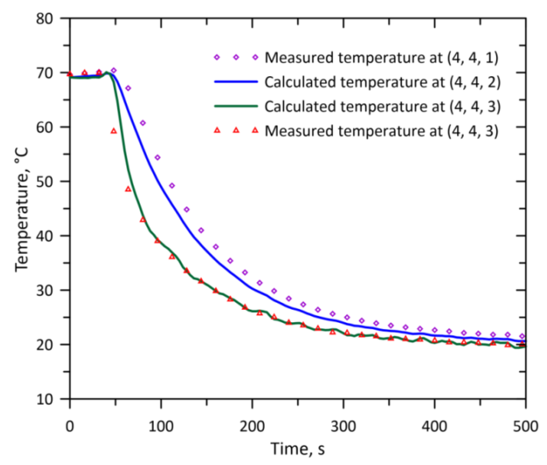
The four control points at which the measured temperature was compared with the calculated temperature were located as follows: one point on the water-cooled surface; one point at a distance of 11.7 mm from the cooled surface; and two points at a distance of 23.3 mm from the cooled surface. Figure 6 depicts the temperature measured at node (4,4,1) on the rear heated surface, the temperature calculated at node (4,4,2) at distance z = Δz from the insulated surface, and the calculated and experimental temperature values at node (4,4,3) placed on the exposed sprayed surface. The calculated and measured temperature at node (4,4,3) as well as in other points, exhibited a very good coincidence. The results shown in Figure 6 were obtained by dividing the thickness of the plate into three control volumes. The heat flux at node (4,4,3) was estimated using three formulas (Equations (7)–(9)). The time changes of the heat flux and heat transfer coefficient determined on the sprayed surface at node (4,4,3) are illustrated in Figure 7.
The analysis of the results presented in Figure 7 shows that Equations (8) and (9) gave almost identical results due to the second-order of the accuracy of Equations (8) and (9). The relative difference between the heat transfer coefficient hIII (Method III) and hI (Method I) when calculating the heat flux from Equations (7) and (9) is:
The maximum value of the relative difference of 23.9% occurs at time t = 88 s (Figure 7).
A comparison of the heat transfer coefficients calculated from Equations (7) and (8) for dividing the thickness of the plate into four control volumes in the z-axis direction is shown in Figure 8. The relative difference between the heat transfer coefficients hII and hI was calculated as follows: . The maximum value of this difference was 15.8% (i.e., it decreased by approx. 10% compared to the division of the thickness of the plate into three control volumes). As in the previous case, the maximum difference between the hII and hI coefficients was for the time t = 88 s.
Equation (7) is the most sensitive to the number of control volumes in the z-axis direction. When the heat flux was calculated from Equation (8), and the thickness of the plate was divided into three control volumes, the maximum heat transfer coefficient was 2102.9 W/(m2·K). When the number of control volumes was increased to four, the maximum value was 2105.9 W/(m2·K) (i.e., it changed slightly). Similarly, for Method III, where Equation (9) is used to calculate the heat flux on the cooled surface, a very similar maximum heat transfer coefficient value of 2108.3 W/(m2·K) was obtained. The comparisons showed that good results were obtained when calculating the heat flux on the exposed surface of the plate by the second-order differential quotient (Equation (8)) based on the temperature of the plate in three nodes. In addition, Equation (9) has very good accuracy but requires more temperature measurement points on the heated surface, furthest from the water sprayed one.
5. Conclusions
This paper presented a general method for the determination of temperature, the heat flux, and the heat transfer coefficient at the exposed surface of a thick-walled plane element. The presented method was validated using experimental data. The temperature and heat flux on the water-spray surface were determined using temperature measurements at several dozen points located on the easily accessible insulated opposite surface of the plate.
The calculations and measurements showed that Methods II and III were more accurate than Method I. They provided very similar time variations of the heat transfer coefficient. In practical applications, the second formula, based on temperatures in three nodes, is more convenient because it requires fewer temperature measurement points on the thermally insulated surface of the plate.
The results of the temperature measurement in internal nodes were compared with the results obtained from the solution of the inverse problem of heat conduction. A very good agreement of the experimental and calculation results was obtained despite the fact that the boundary condition on the surface sprayed with water was identified on the basis of temperature measurements at a large distance from that surface.
The method developed, combined with the method of measuring the transient fluid temperature proposed by Jaremkiewicz, enables the calculation of the heat transfer coefficient at the inner surface of pressure components. Through the precise determination of the fluid temperature and heat transfer coefficient at the inner surface, thermal stresses arising in the pressure component of complicated geometry can be calculated using the finite element method. The proposed method can also be used online to determine thermal stresses at concentration points, for example, at the edges of openings.
Another advantage of the method is the ease of practical application. To determine the local heat transfer coefficient of the internal surface, the temperature of the insulated external surface over a small area is measured.
High stability and accuracy of the inverse heat conduction problem are achieved by using digital filters to eliminate accidental measurement errors from the temperatures measured on the insulated external surface.
Author Contributions
Conceptualization, J.T.; Methodology, J.T.; Validation, M.J.; Investigation, M.J.; Writing—original draft preparation, J.T.; Visualization, M.J.; Supervision, J.T. All authors have read and agreed to the published version of the manuscript.
Funding
This research received no external funding.
Conflicts of Interest
The authors declare no conflicts of interest.
References
Pang, L.; Yi, S.; Duan, L.; Li, W.; Yang, Y. Thermal stress and cyclic stress analysis of a vertical water-cooled wall at a utility boiler under flexible operation. Energies2019, 12, 1170. [Google Scholar] [CrossRef]
Riboldi, L.; Nord, L.O. Lifetime assessment of combined cycles for cogeneration of power and heat in offshore oil and gas installations. Energies2017, 10, 744. [Google Scholar] [CrossRef]
Taler, J.; Zima, W.; Ocłoń, P.; Grądziel, S.; Taler, D.; Cebula, A.; Jaremkiewicz, M.; Korzeń, A.; Cisek, P.; Kaczmarski, K.; et al. Mathematical model of a supercritical power boiler for simulating rapid changes in boiler thermal loading. Energy2019, 175, 580–592. [Google Scholar] [CrossRef]
Oliver, S.J.; Mostafavi, M.; Hosseinzadeh, F.; Pavier, M.J. Redistribution of residual stress by thermal shock in reactor pressure vessel steel clad pressure vessels and piping. Int. J. Press. Vessel. Pip.2019, 169, 37–47. [Google Scholar] [CrossRef]
Raafat, E.; Nassef, A.; El-Hadek, M.; El-Megharbel, A. Fatigue and thermal stress analysis of submerged steel pipes using ANSYS software. Ocean Eng.2019, 193, 106574. [Google Scholar] [CrossRef]
Guo, X.; Sun, W.; Becker, A.; Morris, A.; Pavier, M.; Flewitt, P.; Tierney, M.; Wales, C. Thermal and Stress Analysis of a novel coated steam dual pipe system for use in advanced ultra-supercritical power plant. Int. J. Press. Vessel. Pip2019, 176, 103933. [Google Scholar] [CrossRef]
Kwon, H.G.; Hwang, S.D.; Cho, H.H. Measurement of local heat/mass transfer coefficients on a dimple using naphthalene sublimation. Int. J. Heat Mass Transf.2011, 54, 1071–1080. [Google Scholar] [CrossRef]
Che, M.; Elbel, S. An experimental method to quantify local air-side heat transfer coefficient through mass transfer measurements utilizing color change coatings. Int. J. Heat Mass Transf.2019, 144, 118624. [Google Scholar] [CrossRef]
Gultekin, D.H.; Gore, J.C. Measurement of heat transfer coefficients by nuclear magnetic resonance. Magn. Reson. Imaging2008, 26, 1323–1328. [Google Scholar] [CrossRef] [PubMed]
Joachimiak, M.; Joachimiak, D.; Ciałkowski, M.; Małdziński, L.; Okoniewicz, P.; Ostrowska, K. Analysis of the heat transfer processes of the cylinder heating in the heat-treating furnace on the basis of solving the inverse problem. Int. J. Therm. Sci.2019, 145, 105985. [Google Scholar] [CrossRef]
Zhu, K.; Li, Y.; Ma, Y.; Wang, J.; Wang, L.; Xie, F. Cool down performance and induced thermal stress distribution in criogenic tank. Appl. Therm. Eng.2018, 141, 1009–1019. [Google Scholar] [CrossRef]
Hibbeler, R.G. Mechanics of Materials, 10th ed.; Pearson: London, UK, 2016; ISBN 978-0134319650. [Google Scholar]
Jaremkiewicz, M.; Taler, D.; Sobota, T. Measurement of transient fluid temperature. Int. J. Therm. Sci.2015, 87, 241–250. [Google Scholar] [CrossRef]
Jaremkiewicz, M.; Taler, D.; Dzierwa, P.; Taler, J. Determination of transient fluid temperature and thermal stresses in pressure thick-walled elements using a new design thermometer. Energies2019, 12, 222. [Google Scholar] [CrossRef]
Jaremkiewicz, M. Accurate measurement of unsteady state fluid temperature. Heat Mass Transf.2017, 53, 887–897. [Google Scholar] [CrossRef]
Jaremkiewicz, M.; Dzierwa, P.; Taler, D.; Taler, J. Monitoring of transient thermal stresses in pressure components of steam boilers using an innovative technique for measuring the fluid temperature. Energy2019, 175, 139–150. [Google Scholar] [CrossRef]
Taler, J. Identification of Thermal Flow Processes in Theory and Practice; Zakład Narodowy im. Ossolińskich: Wrocław, Poland, 1995; ISBN 83-04-04276-2. [Google Scholar]
Taler, J.; Dzierwa, P.; Jaremkiewicz, M.; Taler, D.; Kaczmarski, K.; Trojan, M. Thermal stress monitoring in thick-walled pressure components based on the solutions of the inverse heat conduction problems. J. Therm. Stress.2018, 41, 1501–1524. [Google Scholar] [CrossRef]
Taler, J.; Dzierwa, P.; Taler, D.; Jaremkiewicz, M.; Trojan, M. Monitoring of Thermal Stresses and Heating Optimization Including Industrial Applications; Nova Science Publishers: New York, NY, USA, 2016; ISBN 978-1-63485-367-5. [Google Scholar]
Taler, J.; Duda, P. Solving Direct and Inverse Heat Conduction Problems, 1st ed.; Springer: Berlin, Germany, 2006; ISBN 978-3-540-33470-X. [Google Scholar]
Taler, J. A semi-numerical method for solving inverse heat conduction problems. Heat Mass Transf.1996, 31, 105–111. [Google Scholar] [CrossRef]
Taler, D.; Taler, J. Optimum heating of thick plate. Int. J. Heat Mass Transf.2009, 52, 2335–2342. [Google Scholar] [CrossRef]
Figure 1.
External dimensions of the flat plate and indication of the start of the coordinate system: (a) general view, (b) plate view from above, and (c) side view of the plate.
Figure 1.
External dimensions of the flat plate and indication of the start of the coordinate system: (a) general view, (b) plate view from above, and (c) side view of the plate.
Figure 2.
Dividing the plate into (a) three and (b) four control volumes layers on the slab thickness.
Figure 2.
Dividing the plate into (a) three and (b) four control volumes layers on the slab thickness.
Figure 3.
View of the planes on which the nodes of the control volume are located: (a) external insulated surface with marked points at which temperature is measured; (b) surface z = Δz; (c) exposed slab surface z = 2Δz; (d) cross-section through the center of the slab with marked nodes.
Figure 3.
View of the planes on which the nodes of the control volume are located: (a) external insulated surface with marked points at which temperature is measured; (b) surface z = Δz; (c) exposed slab surface z = 2Δz; (d) cross-section through the center of the slab with marked nodes.
Figure 4.
Dividing the plate into four control volumes in the z-axis direction: (a) cross-section through the center of the slab with marked nodes; (b) plane z = 3Δz.
Figure 4.
Dividing the plate into four control volumes in the z-axis direction: (a) cross-section through the center of the slab with marked nodes; (b) plane z = 3Δz.
Figure 5.
Spray cooling stand for thick-walled, electrically heated plate: (a) cross-section of the stand; (b) cross-section of the water-cooled plate; (c) an isometric view showing the holes in the top plate where the water spray nozzles are located: 1—thick plate; 2—electrical silicone heater; 3—thermal insulation; 4—jacket thermocouples; 5—water spray nozzles; 6—upper plate in which the nozzles are mounted; 7—hole for mounting the nozzle; 8—cooling water distributor; 9—connection spigot.
Figure 6.
Calculated and measured temperature values on the exposed slab surface at the point (4,4,3).
Figure 6.
Calculated and measured temperature values on the exposed slab surface at the point (4,4,3).
Figure 7.
Time variations of heat flux and heat transfer coefficient on the cooled surface when dividing the thickness of the plate into three control volumes.
Figure 7.
Time variations of heat flux and heat transfer coefficient on the cooled surface when dividing the thickness of the plate into three control volumes.
Figure 8.
Time variations of the heat flux and heat transfer coefficient on the cooled surface when dividing the thickness of the plate into four control volumes.
Figure 8.
Time variations of the heat flux and heat transfer coefficient on the cooled surface when dividing the thickness of the plate into four control volumes.
Jaremkiewicz, M.; Taler, J.
Online Determining Heat Transfer Coefficient for Monitoring Transient Thermal Stresses. Energies2020, 13, 704.
https://doi.org/10.3390/en13030704
AMA Style
Jaremkiewicz M, Taler J.
Online Determining Heat Transfer Coefficient for Monitoring Transient Thermal Stresses. Energies. 2020; 13(3):704.
https://doi.org/10.3390/en13030704
Chicago/Turabian Style
Jaremkiewicz, Magdalena, and Jan Taler.
2020. "Online Determining Heat Transfer Coefficient for Monitoring Transient Thermal Stresses" Energies 13, no. 3: 704.
https://doi.org/10.3390/en13030704
APA Style
Jaremkiewicz, M., & Taler, J.
(2020). Online Determining Heat Transfer Coefficient for Monitoring Transient Thermal Stresses. Energies, 13(3), 704.
https://doi.org/10.3390/en13030704
Note that from the first issue of 2016, this journal uses article numbers instead of page numbers. See further details here.
Article Metrics
No
No
Article Access Statistics
For more information on the journal statistics, click here.
Multiple requests from the same IP address are counted as one view.
Jaremkiewicz, M.; Taler, J.
Online Determining Heat Transfer Coefficient for Monitoring Transient Thermal Stresses. Energies2020, 13, 704.
https://doi.org/10.3390/en13030704
AMA Style
Jaremkiewicz M, Taler J.
Online Determining Heat Transfer Coefficient for Monitoring Transient Thermal Stresses. Energies. 2020; 13(3):704.
https://doi.org/10.3390/en13030704
Chicago/Turabian Style
Jaremkiewicz, Magdalena, and Jan Taler.
2020. "Online Determining Heat Transfer Coefficient for Monitoring Transient Thermal Stresses" Energies 13, no. 3: 704.
https://doi.org/10.3390/en13030704
APA Style
Jaremkiewicz, M., & Taler, J.
(2020). Online Determining Heat Transfer Coefficient for Monitoring Transient Thermal Stresses. Energies, 13(3), 704.
https://doi.org/10.3390/en13030704
Note that from the first issue of 2016, this journal uses article numbers instead of page numbers. See further details here.


