1. Introduction
Utility scale solar power capacity continues to have worldwide growth with a total installed capacity of 180 GW at the end of 2018 [
1]. As the capacity of solar power increases, accurate short-term solar power forecasts are becoming increasingly important to maintain grid reliability and minimize use of unnecessary fossil fuel-based reserves. Numerous studies have examined various solar power forecasting techniques, which have been broadly discussed in several book chapters and review papers including [
2,
3,
4,
5,
6,
7]. Forecasting solar power depends upon first identifying the diurnal pattern of irradiance at a given location, then determining the amount of irradiance attenuated from clouds and aerosols such as dust. The diurnal pattern of irradiance is a well understood geometric calculation; however, the cloud growth and evolution is a dynamic process that must be well predicted to capture the irradiance reaching the solar panels at the earth’s surface.
Various algorithms have different predictive ability for cloud growth and evolution at different forecast lead times. At very short time scales, large utility scale solar power farms that have a total sky imager (TSI) or upward facing camera may be able to extract cloud information from the TSI and advect the clouds over the domain of the solar farm [
8]. The predictive skill depends inherently on the height of the cloud and the prevailing wind speed but is generally limited to 15 min or less of forecast lead time.
In addition to upward facing imagery, satellite-based techniques can also be used in the short time scales of minutes to hours to identify clouds and advect them forward in time. Satellites have a much wider viewing lens than upward facing cameras on the ground; therefore, the inherent forecast capability extends further than TSI-based techniques. However, the resolution of satellite-based techniques is substantially less than TSI so some information on the clouds over an area can be lost with satellite-based techniques. In [
9], a satellite-based cloud advection technique with advancements to shadowing, parallax removal and including wind speeds at different vertical levels is used for more accurate cloud motion estimates.
In addition to TSI or satellite-based techniques of cloud advection, artificial intelligence and machine learning techniques trained on observations and numerical weather prediction (NWP) output have shown improved forecast skill in the forecast lead time frame of minutes to several hours. Machine learning techniques can learn non-linear relationships among predictors, which in the case of solar power forecasting are data variables that are relevant for modeling cloud growth and decay. Although one would not expect machine learning techniques to capture the movement, growth and decay of individual clouds, the machine learning techniques are trained to predict the amount and variability of solar irradiance that represent the overall effect of clouds on surface irradiance. Additionally, by normalizing the irradiance by the top of atmosphere (TOA) irradiance, the resulting clearness index value quantifies the amount of surface irradiance attenuated by both clouds and aerosols. Therefore, when the machine learning model is given a time series of historical clearness index “observations” and is trained to predict the future clearness index values, the model inherently incorporates the aerosol loading and attenuation, as well as the dust accumulation on the panels, into the prediction. Machine learning can bridge the gap between persistence and physical-based NWP models by learning the relationships among predictor variables and solar irradiance; however, there are many different machine learning algorithms that can be used and each has its strengths and weaknesses depending on the quality of the training data.
The most common machine learning algorithms for solar irradiance or power prediction are support vector machines (SVM)/support vector regression (SVR) and Artificial Neural Networks (ANNs) with regression trees, random forest, and gradient boosted regression trees used less frequently [
10]. Although the growth of SVM and machine learning has increased since 2000, the specific use of ANNs has had the steepest increase in publications per year as evidenced by Figure 6 in [
10]. A recent review by [
11] examined 68 off-the-shelf machine learning algorithms to predict solar irradiance. They found that tree-based methods were superior in long-term average normalized root mean square error (nRMSE) under all-sky conditions, whereas ANN and SVMs performed better under certain conditions. It was also stated in [
11] that “daily evaluation results showed how forecast performance of a method could change with sky conditions.” Similarly, [
12] compared eleven different statistical and machine learning techniques for predicting solar irradiance in three different climates with weak, medium and high variability of solar irradiance and found differences in optimal model choice depending on site variability. In the weak variability climate, auto-regressive moving average (ARMA) models and ANNs performed the best, in medium variability the ARMA and bagged regression trees performed the best, and in high variability the bagged regression tree and random forest approaches performed the best. Evidently, the choice of model depends upon the solar irradiance variability, which in turn depends on the underlying meteorological phenomena causing cloud movement, growth and dissipation.
In order to capture the inherent differences in predictive skill depending on the underlying variability, recent research has examined hybrid methods that combine unsupervised learning with supervised learning to improve the overall forecasting skill. Work by McCandless et al. [
13,
14] combine the unsupervised machine learning technique, k-means clustering, to first identify the statistical cloud regime, with ANNs applied to each regime independently. The results showed a substantial improvement from 15-min to 3-h lead time for solar irradiance prediction using the regime-dependent artificial neural network (RD-ANN), including an improvement over an ANN trained on all data.
In addition to machine learning-based nowcasting techniques, numerical weather prediction (NWP) models tuned specifically for solar irradiance forecasting, such as WRF-Solar, have been shown to have skill in the forecast lead times greater than a couple of hours out to many days [
15,
16]. Therefore, the machine learning algorithms should also test including NWP forecasts as inputs into the nowcasting models in order to optimize forecast error from minutes to hours ahead. This would allow the algorithm to capture the potential improvement in forecast accuracy gained by physics-based NWP models for lead times when forecast skill from models trained only on current and historical observations decreases.
This work aims to compare the solar power forecasting performance of model tree-based methods that have implicit regime-based models to explicit regime separation methods that utilize both unsupervised and supervised machine learning techniques. Each solar forecasting problem ultimately depends on the complexity of the underlying meteorological phenomena causing varying levels of solar irradiance variability and the quality and quantity of data available for building a statistical or machine learning based model. This study evaluates the solar forecasting performance of the implicit and explicit regime identification machine learning methods on data at a renewable energy plant at the Shagaya Renewable Energy Park in Kuwait where clear skies predominate, with occasional clouds. Dust buildup and aerosol attenuation occur frequently. Additionally, this study evaluates using surface observations and NWP output in order to identify regimes and as inputs to the machine learning methods for a systematic test of the methods from 15-min to 345-min forecast lead time. The regime-dependent models go through a comprehensive sensitivity study to determine the optimal parameter and hyperparameter settings to minimize the forecast error on test data with final results presented from tests on an independent validation dataset.
2. Data
The observed data used in this study is from the Shagaya Renewable Energy Park in Kuwait, which is a renewable energy plant under development with plans to install up to 5 GW of capacity by 2027 [
17]. Shagaya, Kuwait is located in the western area of the country and is dominated by a dry, desert climate. The data available for this study is from the time period of Sept 1, 2017 through May 31, 2019. The observation station is located at latitude 29.2044° and longitude 47.0528° at an elevation of 242-m above sea level. Details of the site and its equipment is provided by Al-Rasheedi et al. [
18]. The station reports data in 5-min intervals that are averaged to 15-min intervals to match the forecast interval of the NWP model output, also used as input for the machine learning models. The variables observed at 3-m height are the temperature, relative humidity, Global Horizontal Irradiance (GHI), rain accumulation and the variables observed at 4-m height are the wind speed and wind direction. There are also four panel temperature observations that are averaged together for an average panel temperature at the photovoltaic solar array. We have included the average panel temperature as a predictor in addition to the ambient air temperature because the panel temperature may inherently capture the dust accumulation on the panels. When there is more dust accumulation, there would be a lower measured GHI and a lower panel temperature. The machine learning models can learn the relationship between the average panel temperature and the ambient air temperature to incorporate the effect of dust accumulation. In addition, when temperatures go over certain thresholds depending on the instrument, the efficiency of pyranometers and solar panels may degree and is an additional benefit of the average panel temperature as a predictor. The GHI values are converted to the clearness index (Kt) by dividing by the extraterrestrial or top-of-atmosphere expected irradiance.
In addition to the observed surface data, NWP forecasts from the DICast
® forecast model are used as inputs into the machine learning model [
19,
20]. The DICast
® forecast system post-processes publicly available model data and observations with a blending system that optimizes the forecast based on each individual model’s recent performance at observation locations [
19,
20]. In this DICast
® forecast instance, three NWP models are blended: the U.S. Global Forecast System (GFS) [
21], Environment Canada’s Global Environmental Mesoscale model (GEM) [
22], and a customized version of the Weather Research and Forecasting (WRF) model [
23]. The DICast
® forecast produces hourly forecasts at the top of every hour that are interpolated to 15-min for GHI, cloud cover, temperature, dewpoint temperature, surface pressure, hub height (76-m) wind speed, and direction. In this study, we focus on each 15-min forecast lead time from 15 min to 6 h.
The DICast
® forecasts, current surface observations, hour of the day, 15-min average solar elevation and azimuth angles, and previous 90 min of 15 min averages of Kt are included in the predictor set used in the machine learning algorithms. The surface observations are 15-min averages with the exception of the U-Wind and V-Wind components that are instantaneous values at the end of the 15-min intervals. The last six 15-min clearness index values are included as predictors in order for the machine learning models to capture the recent trend of the irradiance. The final list of predictors is shown in
Table 1. We removed instances where the GHI is less than 50 W/m
2 in the current and historical (past 90-min) data so that the model is trained only when there is sufficient irradiance to produce meaningful solar power generation. The data are split into 13 sets of four weeks per year. Three of those four weeks are randomly chosen for the training dataset and one week for the validation dataset. This approach preserves the ability to leverage time dependent information from past observations while maintaining the ability to train on all seasons of the year. In order to find the optimal configuration (i.e., determining the optimal hyperparameters such as the number of hidden layers of the artificial neural network) of the models, the training dataset was subset where another six weeks per year were randomly chosen to be held out for configuration testing. The optimal configuration of the models is evaluated using the configuration test dataset, and the optimal models are trained on the complete training dataset to predict the validation dataset.
3. Methods
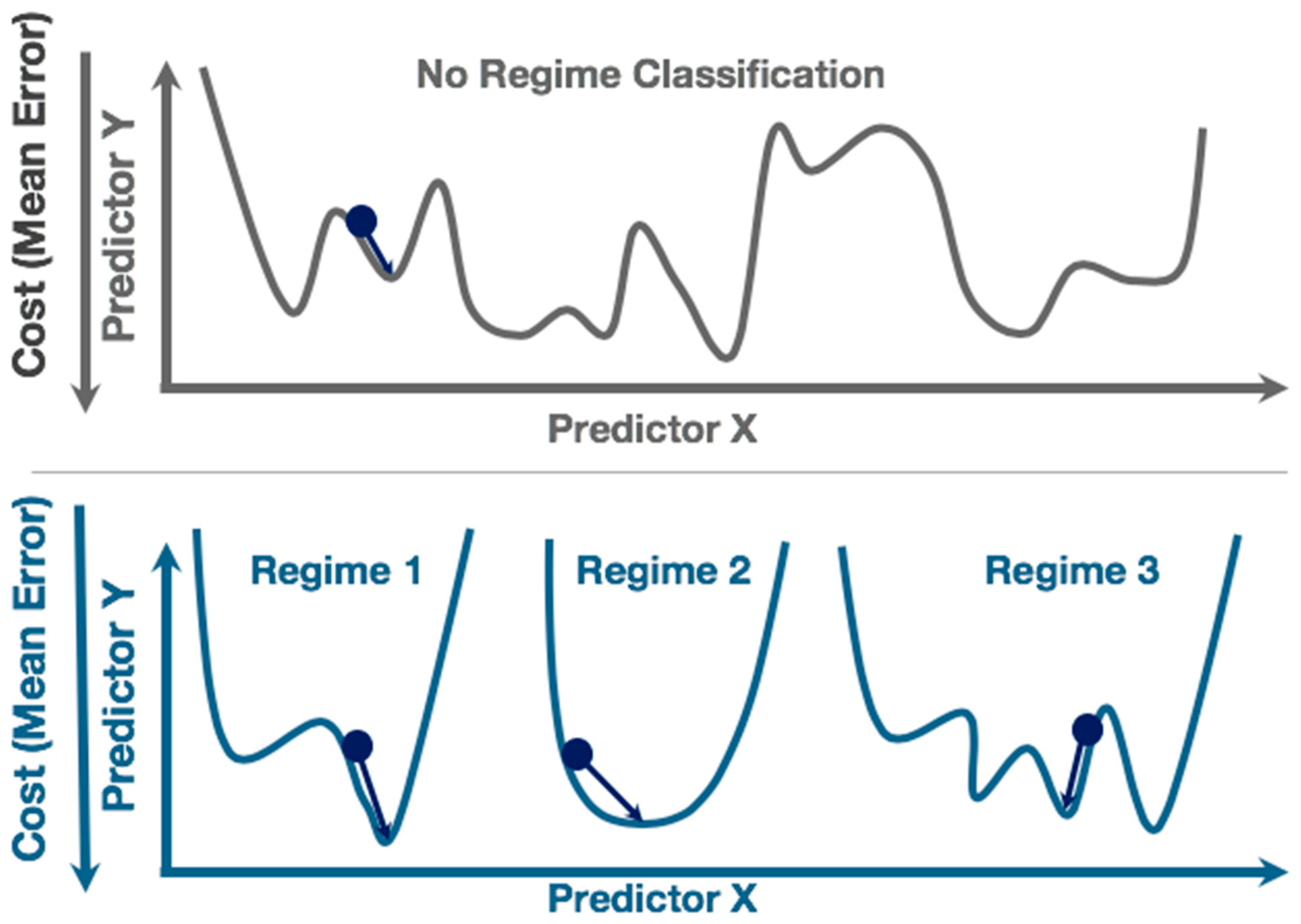
The benefit of the regime-dependent artificial neural network (RD-ANN) approach is to separate the data when the underlying physical relationships between the predictors are expected to differ. In solar irradiance forecasting, we would expect there to be different predictive skill in the case of clear sky compared to partly cloudy cumulus sky conditions. Therefore, the goal of the RD-ANN approach is to separate the data so that each ANN is able to maximize the predictive skill by minimizing the error in the cost function in each of the training data subsets. A conceptual diagram of the underlying machine learning algorithm training is shown in
Figure 1, where an ANN may not be able to find the global minimum in the cost function for the ANN trained without regime classification (top), but is able to find a lower error with more global minima in each of the regimes independently (bottom). In an operational setting, the system would use one model to select the current regime and another model to predict the variable of interest.
In order to classify regimes, the unsupervised learning technique k-means clustering is used on three different data subsets. The k-means clustering technique groups data by separating each sample into a number (k) of different groups. This is accomplished by minimizing the within-cluster sum-of-squared differences from the mean of the cluster and maximizing the between-cluster sum-of-squared differences from the cluster means, as was applied in [
13,
14] for solar irradiance prediction. Three different data subsets used for regime identification capture different aspects of the forecast situation: surface observations, DICast
® forecasts, and the six most recent 15-min averaged clearness index values. The surface observation subset includes the air temperature, relative humidity, u-wind, v-wind, GHI, and average panel temperature. The DICast
® forecast subset includes the clearness index, cloud cover, air temperature, dewpoint temperature, and surface pressure. L2-normalization is performed on each of the three subsets for regime identification before applying the k-means clustering algorithm with the Python Sklearn Clustering module KMeans with a range from two to five clusters. In order to determine the optimal configuration, a sensitivity study first evaluated the optimal configuration of the artificial neural network model.
The ANN is a supervised machine learning approach that is modeled after how brains learn from the information provided to them. The ANN used here is a feed-forward multi-layer perceptron that is trained with a back-propagation algorithm [
24,
25]. We utilize TensorFlow’s Keras model for the ANN and in the final evaluation we test both the regime-dependent ANN as well as an ANN trained on the entire training dataset. In a sensitivity study evaluating different ANN configurations of hidden layers and neuron combinations, learning rates, activation functions, and learning rates, we determined that the optimal configuration of the ANN was the following: one hidden layer of 10 neurons, a Rectified Linear Unit (ReLU) activation function with learning rate of 0.0001, the Adam optimizer, and mean absolute error (MAE) loss function. In order to determine the optimal choice of regime subset and number of regimes, a sensitivity study evaluated the performance of the RD-ANN methods for a range of two to five regimes in each regime subset. The results are shown in
Table 2 for three forecast lead times tested: 60-min, 180-min, and 300-min. The optimal regime identification subset was subset 1, the surface observations, due to showing the lowest MAE at all lead times. Ultimately, we opted to use the configuration with four regimes (k = 4) since that had the lowest error on two of the three time periods shown and had the second lowest MAE at the 60-min forecast lead time (0.045) as well. The regime subset comprised of the past history of clearness index observations (set 2 in the table) seemed to perform relatively well based on MAE; however, the k-means clustering tended to group most instances into a single cluster and minimal instances into the other clusters. For example, with five regimes at 180-min forecast lead time the k-means clustering put 1456 instances in the test dataset in one regime and the other three regimes had only 1, 3 and 9 instances. This highlights the fact that in eastern Kuwait there are minimal variations in clearness index, rather the sky tended to be clear the vast majority of the time. In an operational forecasting environment, this system would operate as follows: First, a data subset for the variables k-means we will use (the surface observations) will be created based on the most recent observations. Second, the trained k-means algorithm will be applied to that data subset to determine the current regime. Third, the trained ANN for that specific regime will be applied to make the irradiance prediction.
While we utilize the k-means clustering to explicitly identify regimes and then apply the ANN to capture the non-linear relationships among the predictors in each regime, there are tree-based methods that include inherent regime-identification and capture non-linear relationships. One of these methods is the Cubist model, which is a model tree-based machine learning method that is accomplished as a set of rules [
26,
27]. The Cubist model tree has implicit regime identification because each branch in the tree is a rule, such as the air temperature greater than a specific threshold, determined based on the error in the training data. The model tree in [
27] has a multivariate linear regression model at each leaf, which in this study is configured to predict the clearness index. The final prediction for a given instance from the model tree is a weighted average of the prediction of each leaf in the tree that meets the conditions of the rules for that instance. The weighting of the final prediction by each leaf tends to avoid overfitting any particular smaller subset of the rules that an instance may follow in the path of the tree. Four different Cubist models were implemented for each lead time. The first, CubistObs, uses current observations of temperature, u-wind, v-wind, relative humidity, and Kt, and the previous 90 min of 15-min averages of Kt. The next, Cubist, uses the predictors above; DICast percent cloud cover at generation time; and valid DICast forecast variables Kt, cloud cover, temperature, pressure, and dewpoint temperature. The third, CubistOpt, uses a subset of the available predictors formed by stepwise regression to minimizes MAE of Kt prediction on the training instances. Stepwise regression combines forward selection with backward elimination to sequentially build an optimal minimal set of predictors. Forward selection adds the predictors in order of value added to the predictor set as a whole. An occasional backward elimination step allows for the elimination of variables whose contributions or value may have become obsolete by a subset of other variables which together provide greater value to the prediction. Rather than predefining the predictor set or all lead times, a unique set of predictors is built at each lead time which maximizes predictive performance at that lead time, which is our CubistOpt model. Finally, RDCubist consists of four models at each lead time trained on instances separated by regime resulting from application of the k-means clustering algorithm. The results of the ANN, RD-ANN, CubistObs, Cubist, CubistOpt, and RD-Cubist are compared to both the DICast forecasts of GHI converted to clearness index and the smart persistence technique that uses the most recent clearness index observation as the forecast at all forecast valid times.
4. Results
The results described in this section are on the independent validation dataset of a random 13 weeks per each year.
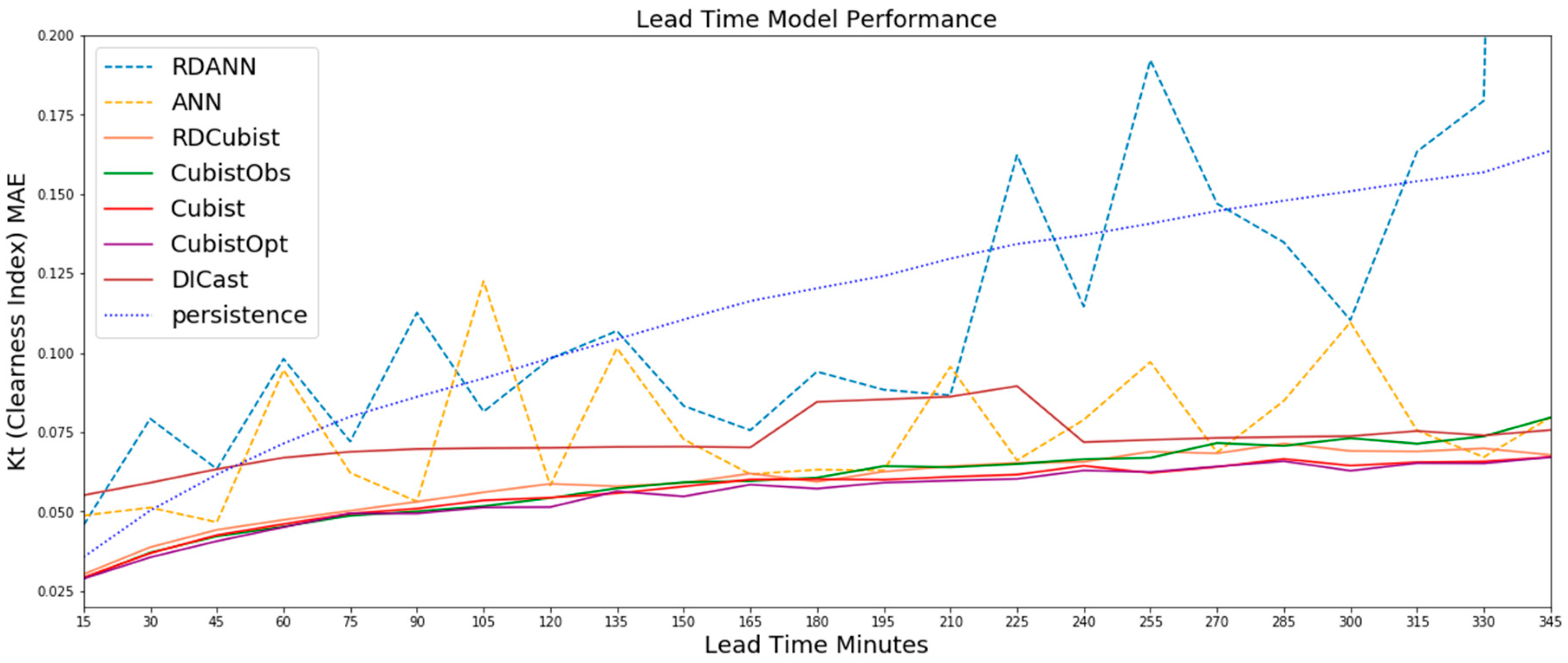
Figure 2 illustrates the Kt MAE for all forecast lead times from 15-min to 345 min for each of the methods tested. In addition to the MAE shown in
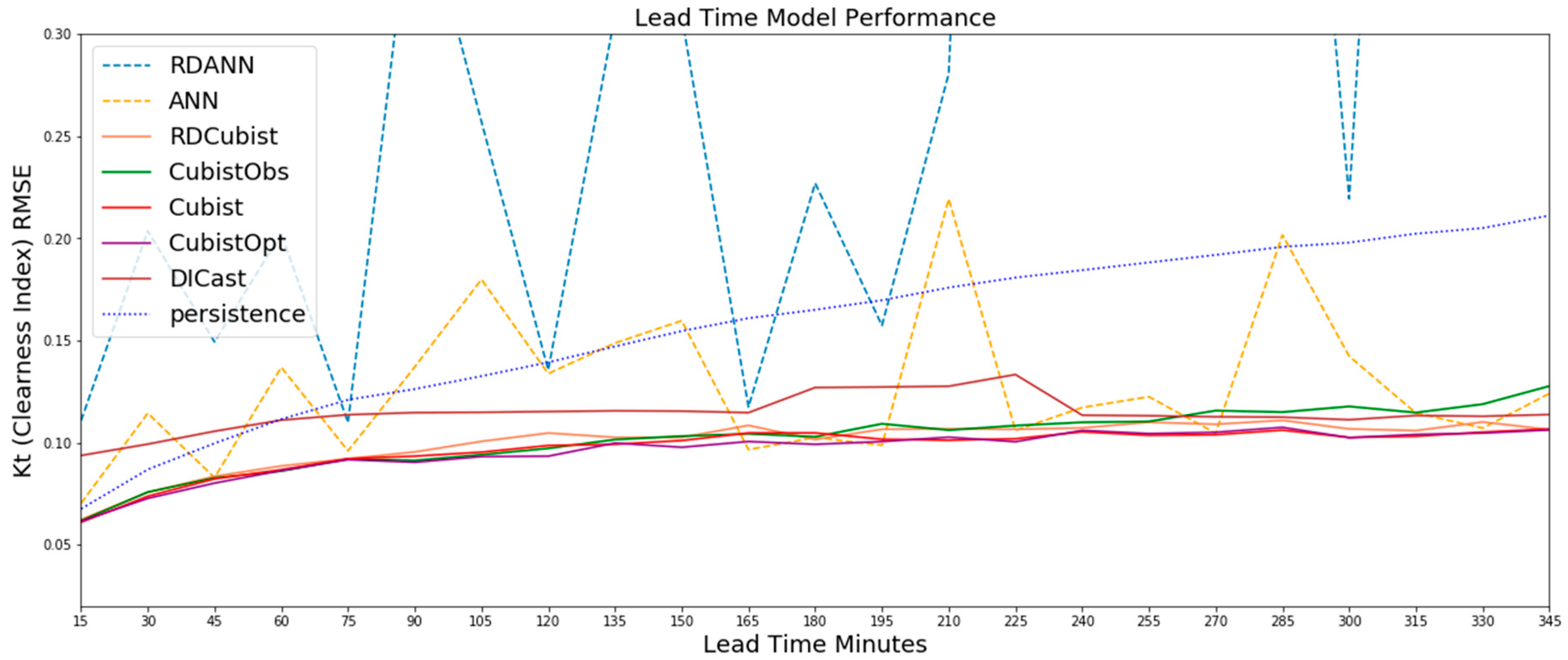
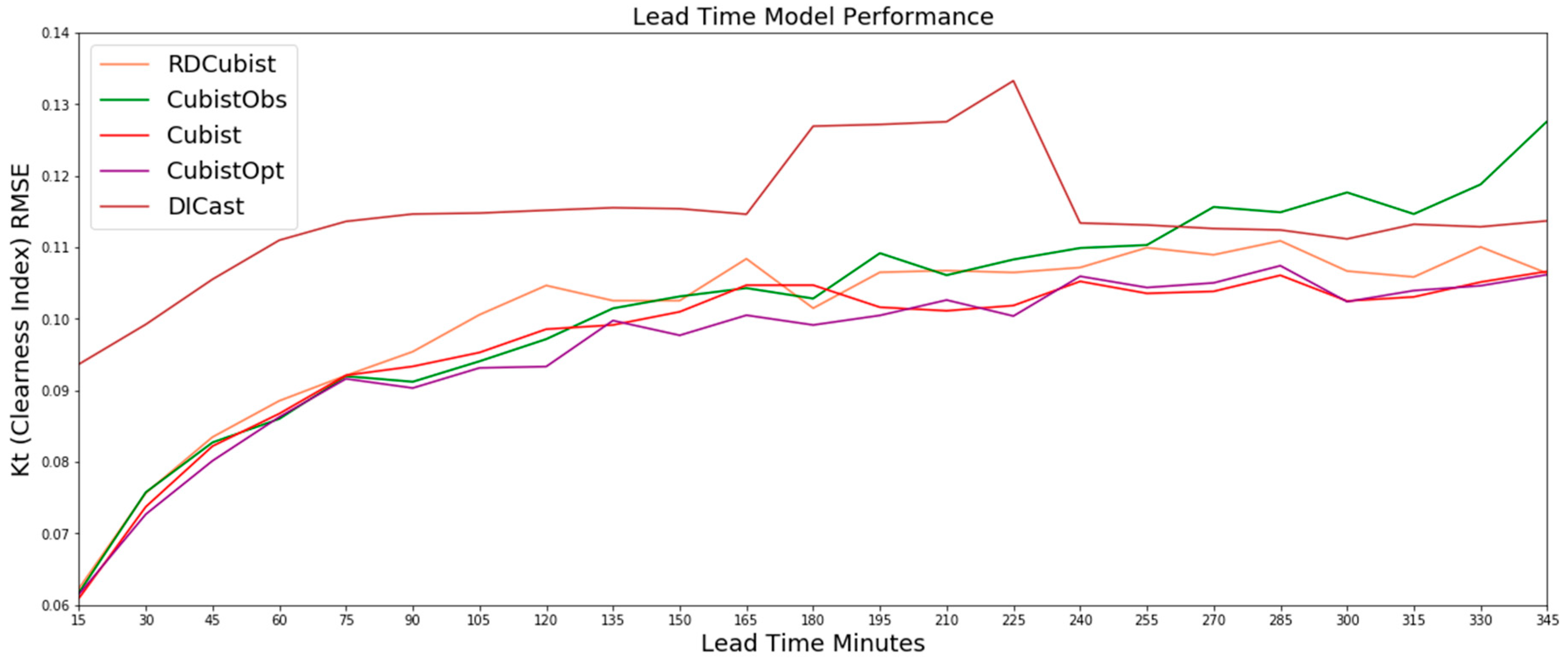
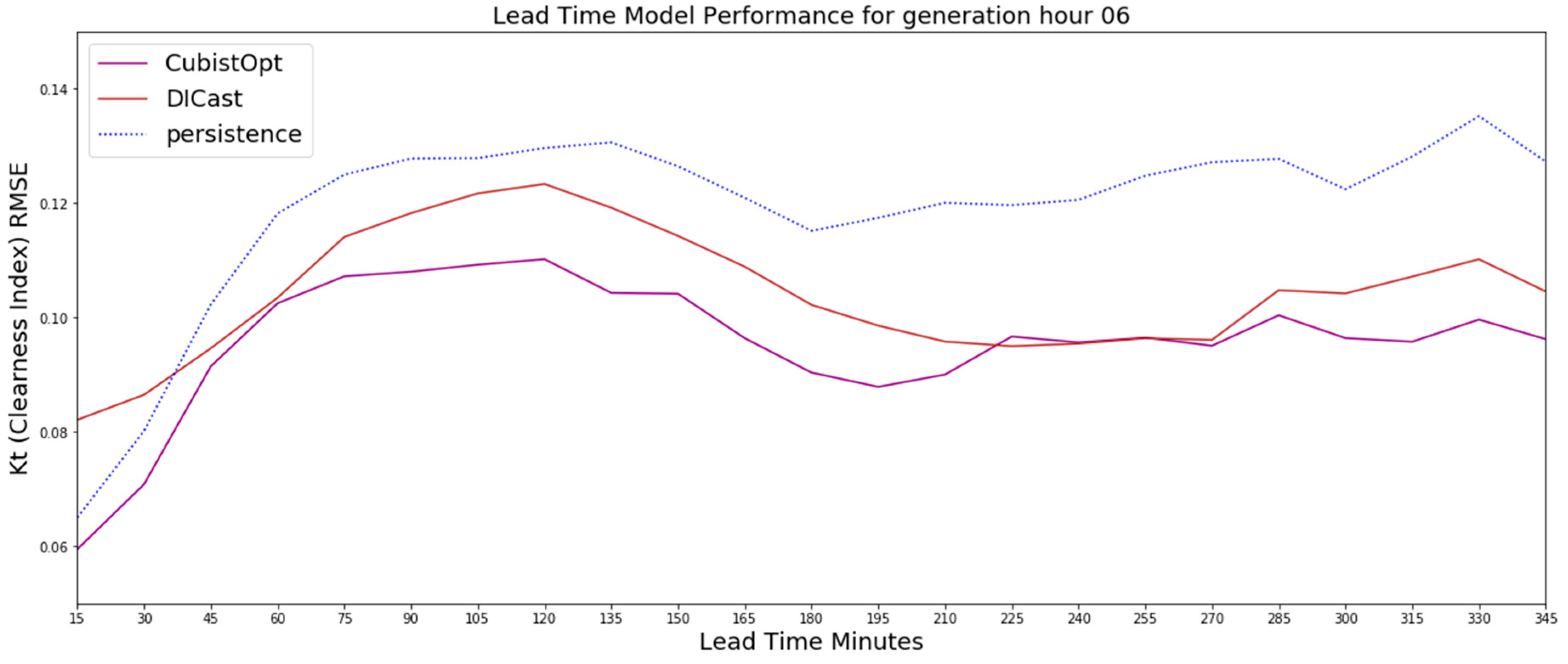
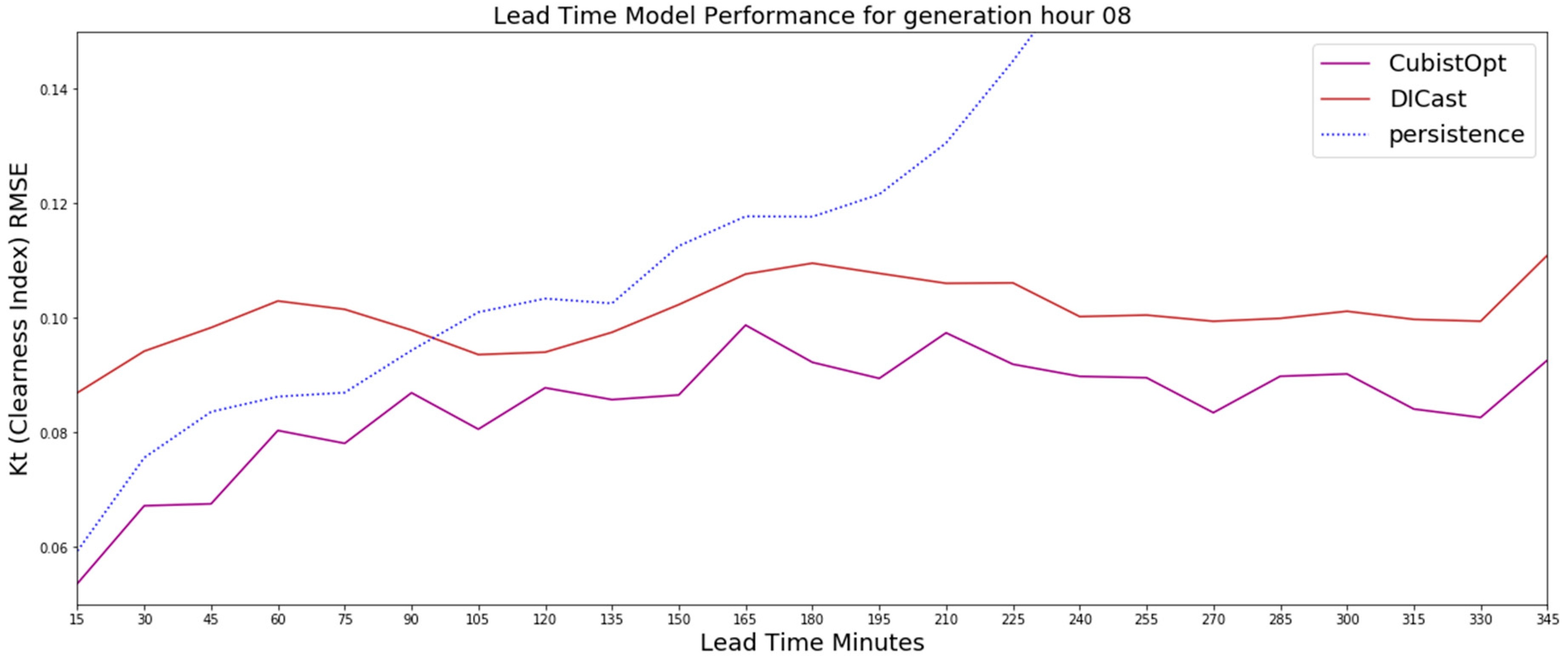
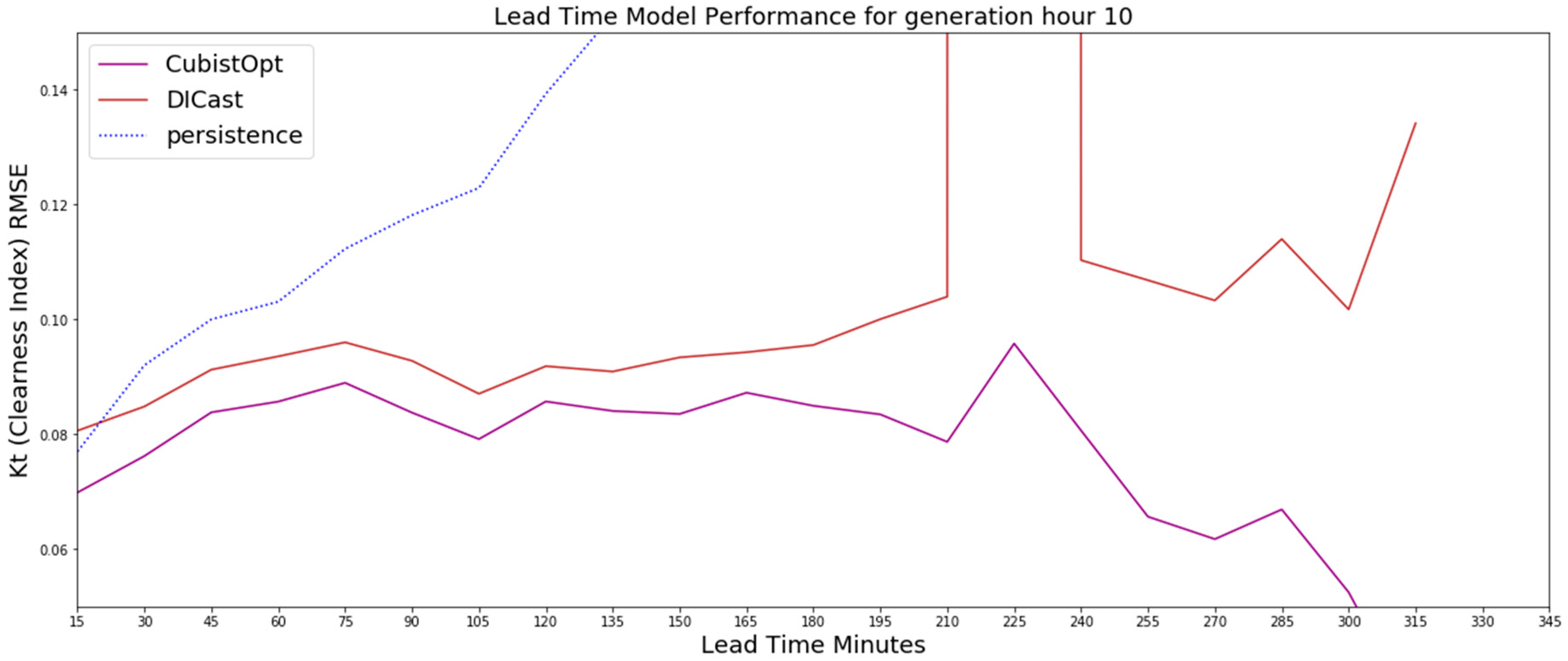
Figure 2, we have included root mean square error (RMSE) plots for
Figure 2,
Figure 3,
Figure 4,
Figure 5 and
Figure 6 as a supplement in
Appendix A. The ANN based approaches are shown in dashed colored lines, the Cubist based approached in solid colored lines and persistence as dotted blue line. The model with the highest error is the RD-ANN model at nearly all lead times. Both the DICast
® and the ANN perform similarly on average, but the ANN has more variability between time steps. Although the ANN was optimally configured on the test dataset, it is likely that the ANN may overfit the training data available and not generalize well. This is also evident in the regime-dependent approach where the RD-ANN method performs worst, potentially a result of subsetting the data where the predictive relationships, or signal, was not more important than the chance relationships, or noise. As described in the methods section, the goal of the RD-ANN approach is to separate the data so that each ANN is able to maximize the predictive skill by minimizing the error in the cost function in each of the training data subsets. In this instance, by subsetting the data we are likely producing subsets without different predictability and therefore ultimately reducing training samples to minimize the cost function error.
While the ANN-based methods have the highest error of the methods tested, the Cubist-based models performed much better with clearness index MAEs ranging from 0.03 to 0.06 over the forecast time period.
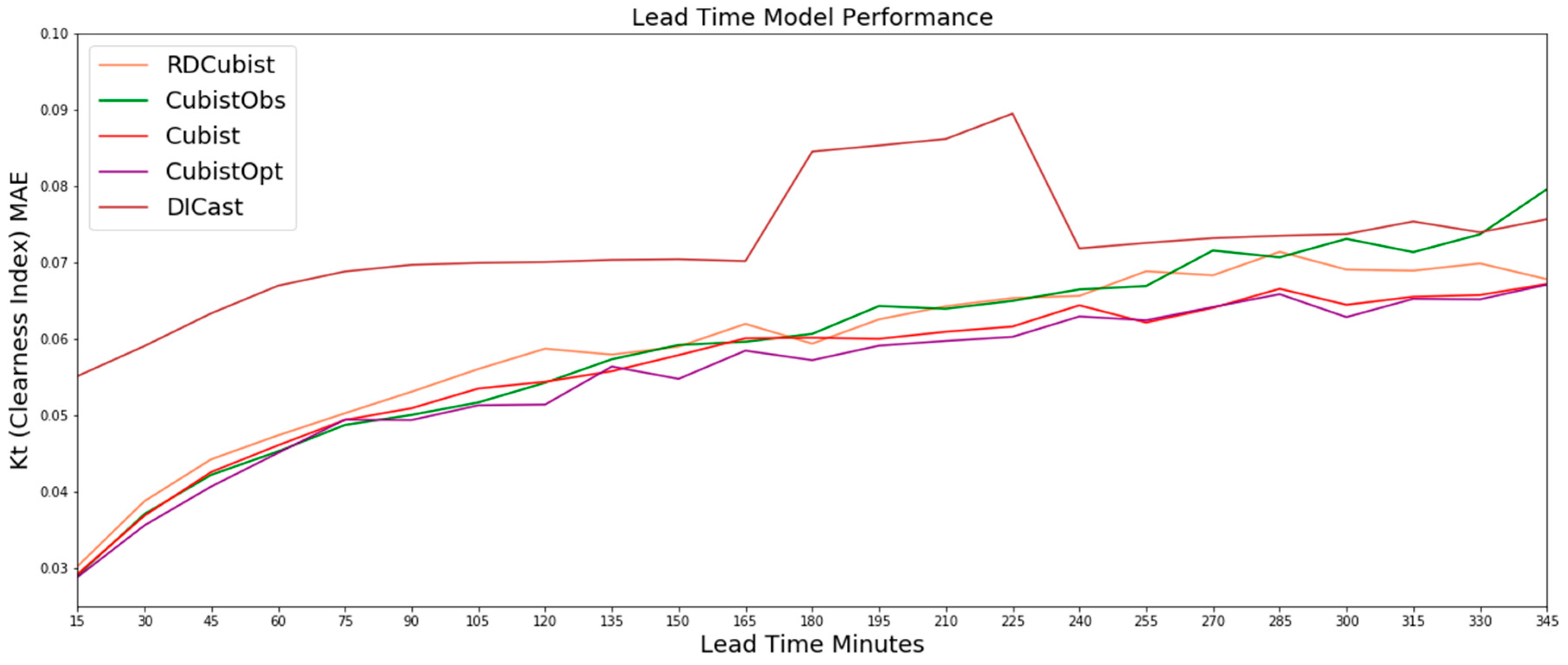
Figure 3 shows the results for the Cubist models as well as the DICast
® forecasts, which better illustrates the differences between the Cubist approaches. The CubistOpt method had slightly lower MAEs on average than the Cubist and RD-Cubist approaches, and the RD-Cubist had the highest MAEs of the three Cubist methods. This is another indication that the k-means approach did not separate the models into meaningful regimes for which the relationship between the predictor and the predictand differed.
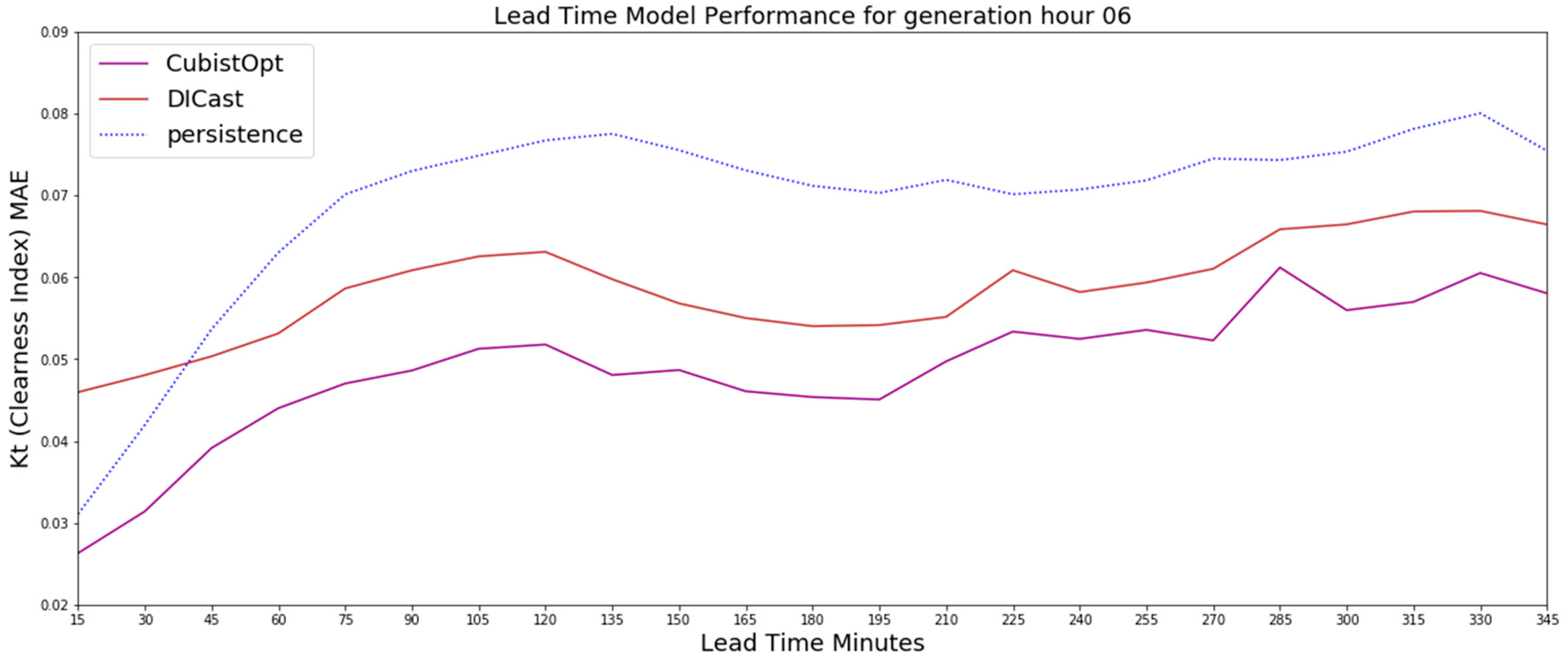
While it is clear the CubistOpt models performed best on average over the testing period, we further examined the error of the CubistOpt models at generation times different from the DICast predictions.
Figure 4 shows the results for the CubistOpt models as well as the DICast forecasts and clearness index persistence at the 06 UTC generation time (i.e., the time at which the DICast model forecasts and the machine learning models were created), which is typically about two hours after sunrise. The CubistOpt (purple line in
Figure 4) method has the lowest error over all time periods. The clearness index persistence is second best for the first 30-min, with the DICast method improving over clearness index persistence after 30-min. Between 30-min and 345-min the CubistOpt method appears to reduce a systematic bias of the DICast model with generally about 0.01 lower Kt error.
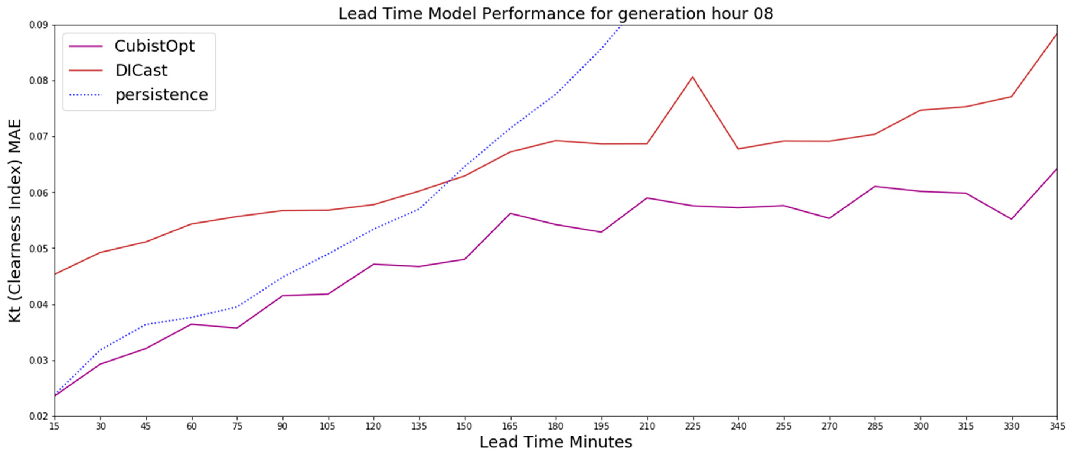
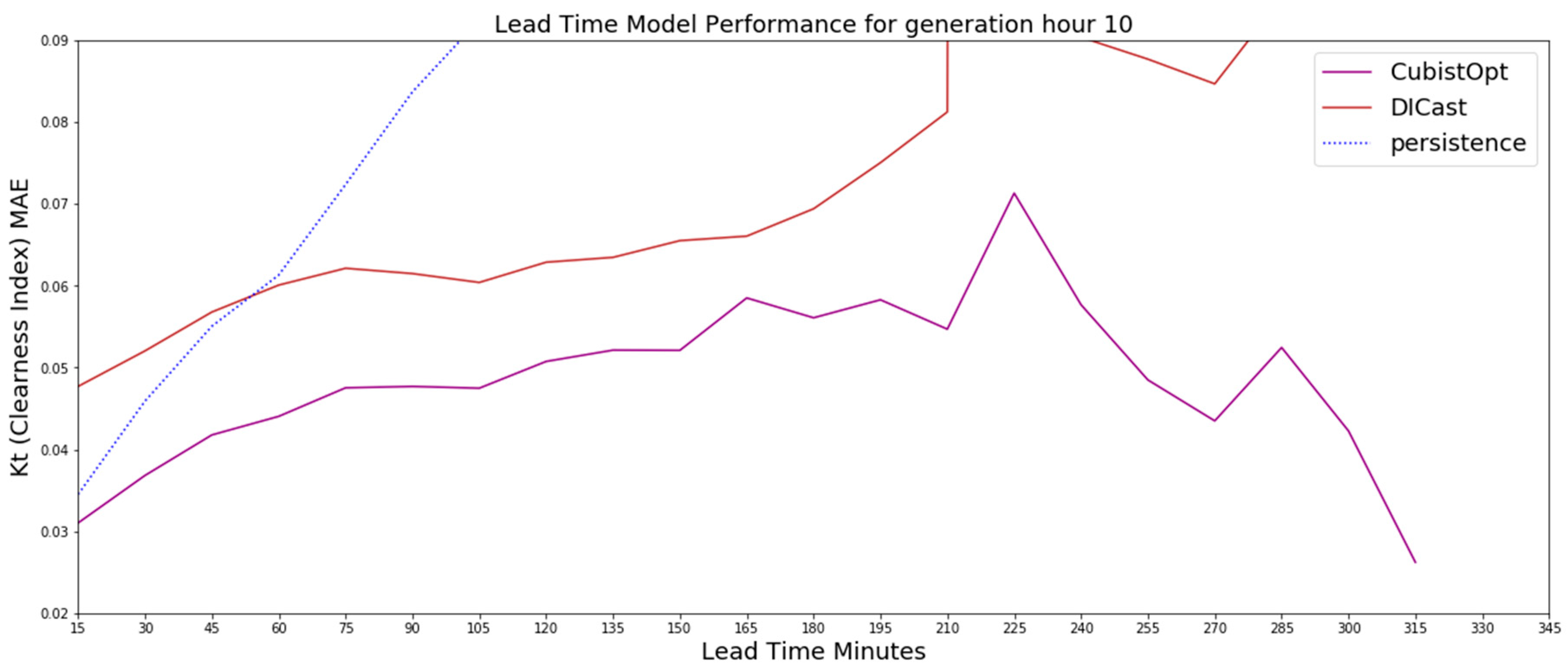
Similar to the 6 UTC generation time forecasts, the 8 UTC and 10 UTC generation time forecasts show the CubistOpt model performs better than clearness index persistence and DICast. For the 8 UTC generation time,
Figure 5, the results show that the clearness index persistence performs second best out until nearly 150-min. After 150-min, the DICast model performs second best. For 10 UTC generation time, which is approximately a generation time around noon local time, the results in
Figure 6 show the clearness index persistence performs better than DICast for approximately 45-min, with DICast performing better after 45-min. The results after about 225-min begin to be affected by low sun angles near sunset, which is evident by diverging errors between the DICast and CubistOpt models. Ultimately the generation time forecasts highlight that the CubistOpt models performs best at all forecast lead times and all DICast generation times.
Results: Time Series Analysis
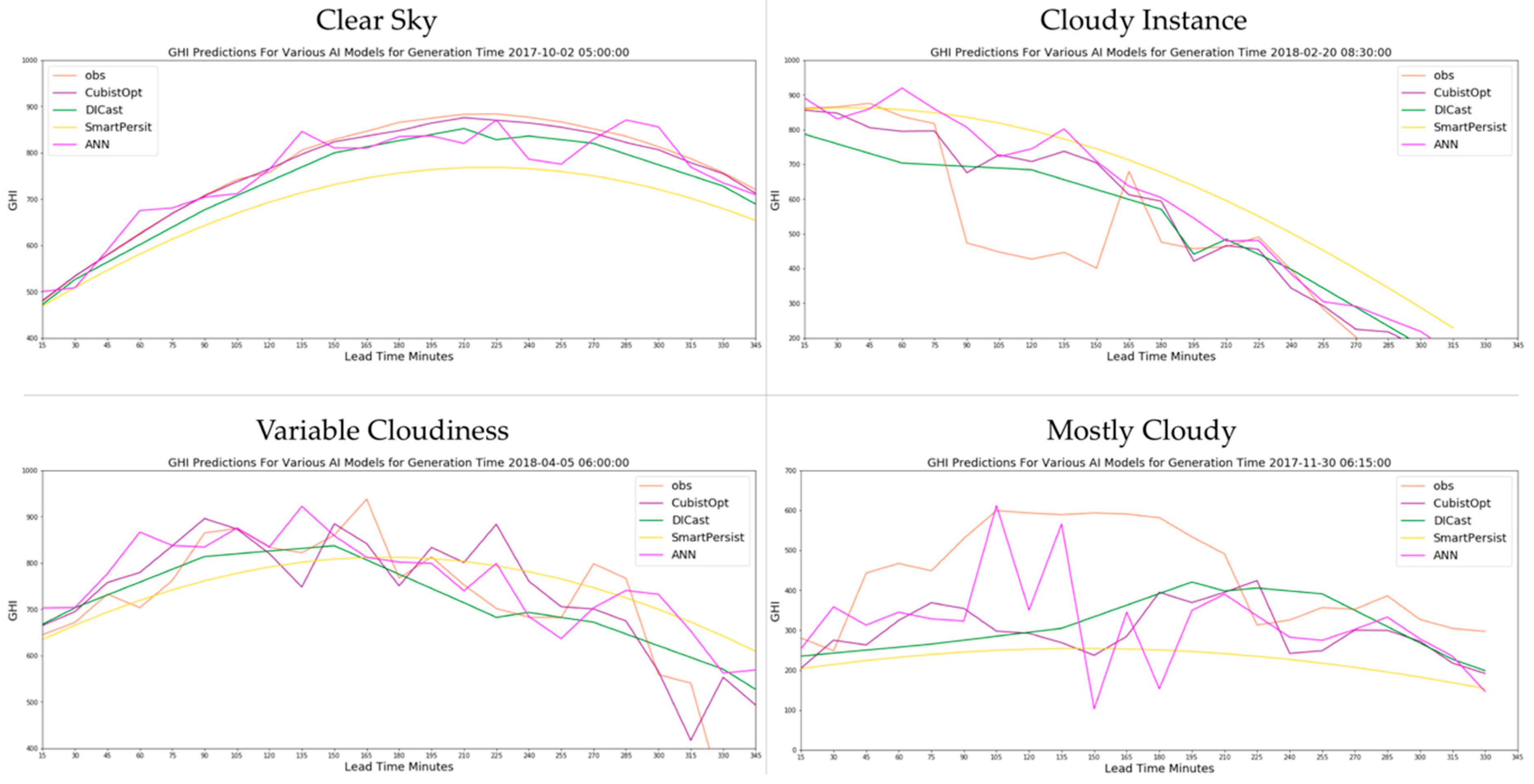
In order to better understand the predictability of the models, we next examine several instances of the best performing models in different weather scenarios. We examine the CubistOpt, DICast, Smart Persistence, and ANN models compared to observations for a clear sky day (
Figure 7: top left), one cloud for one hour (90 min–150 min) during the forecast time period (top right), a variable cloudiness day (bottom left), and a mostly cloudy day (bottom right). During the clear sky conditions, the CubistOpt predictions are closest to the observations throughout the time period, which indicates that the CubistOpt model best captures the predictive skill by reducing the number of predictors in situations with minimal variability. The ANN approach shows more variability in the predictions, which indicates that it is more susceptible to small changes in the DICast forecasts (used as predictors) at the forecast valid time. In the cloudy instance, none of the models are able to capture the cloud moving across the area in the 90 min to 150 min forecast lead time. In the variable cloudiness case, all machine learning based models capture the more uncertain forecast with greater variability in their forecasts compared to the clear sky case. Both the CubistOpt and ANN show variability more similar to the observations than does DICast. Although they may not exactly match the individual variations, they better represent the uncertainty than the DICast forecasts. Finally, in the mostly cloudy case the ANN model does have higher GHI predictions during the beginning of the period where the highest GHI is observed (forecast lead time 105 min–150 min); however, it under-forecasts in the period 150 min–210 min. Generally, all of the models capture the lower than average GHI better than smart persistence.
5. Discussion
In this study, we tested machine learning techniques that include implicit regime identification, explicit regime identification, and a combination of implicit and explicit regime identification methods. We found that the implicit regime identification methods, specifically the Cubist model with a predictor set determined for each lead time by stepwise regression, performed the best on this year of data at the Shagaya Renewable Energy Park in Kuwait. The regime-dependent approaches with explicit regime identification that utilized k-means clustering to independently classify regimes before applying the ANN or the Cubist model degraded the performance of the underlying model. Additionally, the k-means clustering found one dominant cluster when utilizing a time series of Kt observations. This indicates that the underlying meteorology in eastern Kuwait is so strongly dominated by clear sky conditions that an explicit regime-identification approach performs the worst due to minimal cases in the non-clear sky regimes. This study was also limited to less than two years of data that were available at the time of this analysis. This poor performance of the RD-ANN approach compared to the ANN approach appears in conflict with [
13,
14]; however, that study was performed on data from Sacramento, California USA that experiences a more diverse set of cloud (i.e., solar irradiance) regimes.
The Cubist models tested in this study all performed better than the other methods tested, including having lower error than DICast® at all time periods out to nearly six hours forecast lead time. This is likely due to the fact that the Cubist model is a rule-based method, which may allow for more optimal bias correction across the range of forecast lead times. For example, the Cubist model may have a rule that adjusts the forecast if the temperature is greater than a set threshold, and then sequentially adjusts that based on the hour of the day. An additional benefit of the Cubist model over the ANN approach is that the Cubist model is a weighted average of the predictions at each branch in the tree; therefore, the models tends to avoid overfitting better than the ANN approach that does not take an ensemble or weighted average of predictions. Future work will evaluate these approaches in locations that have a significant amount of diverse cloud types and frequencies and a longer data record to determine if the strength of the regime-dependent approaches is fundamentally driven by how diverse and complex the cloud regimes are.
