Impact of Natural Gas Distribution Network Structure and Operator Strategies on Grid Economy in Face of Decreasing Demand


 and
and
Abstract
1. Introduction
- What is the trend of customer development?
- What are the grid-specific factors that influence the profitability of a natural gas grid?
- What are the options for grid operators, regulators and what are the impacts on grid users?
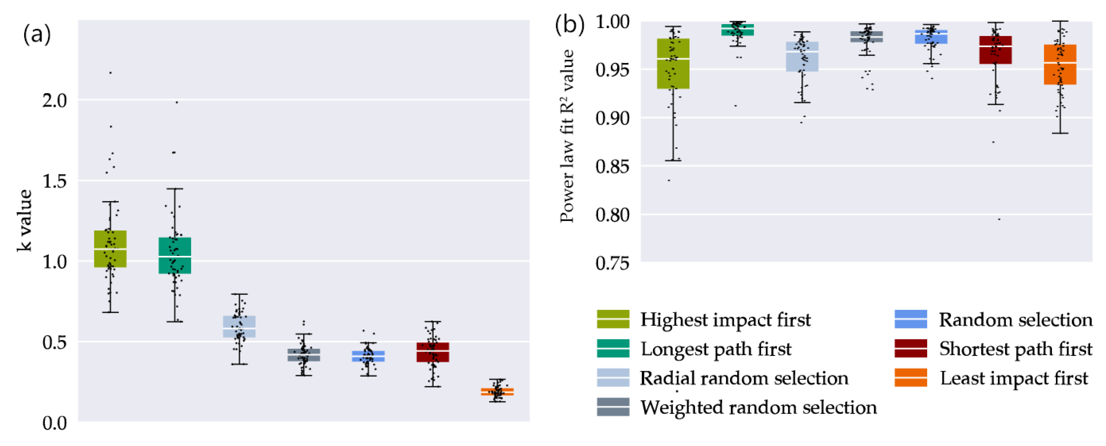
- Within a structural grid analysis, we estimate a functional relationship between required grid length and the amount of customers with a power law approach (Section 3.2.1) for different exit patterns in all grids (Section 4.2). Within a correlation analysis, we identify possible structural parameters for the prediction of the exponent k of the power law, a parameter which determines the disproportionality between grid length and number of customers when they leave the grid (Section 4.3).
- To calculate the total costs of grid operation within an economic analysis, we apply a mixed integer linear optimization model based on a yearly cash flow calculation and transform it into a simplified calculation model considering the functional relationship found in the previous section (Section 3.3.2 and Section 3.3.3). After a validation of the simplified model (Section 4.4.1 and Section 4.4.2), we compare the total costs of operation and resulting grid charges for several exit patterns and DNO investment strategies in Section 4.4.3.
2. Literature Review
2.1. Scenarios for Gas Demand from an International and German Perspective
2.2. Investment Decisions in Building Sector and Their Influence on Grid Economics
2.3. Effects of Grid Structure and Asset Composition on Defection Scenarios
2.4. Economic Factors of Operating a Natural Gas Infrastructure
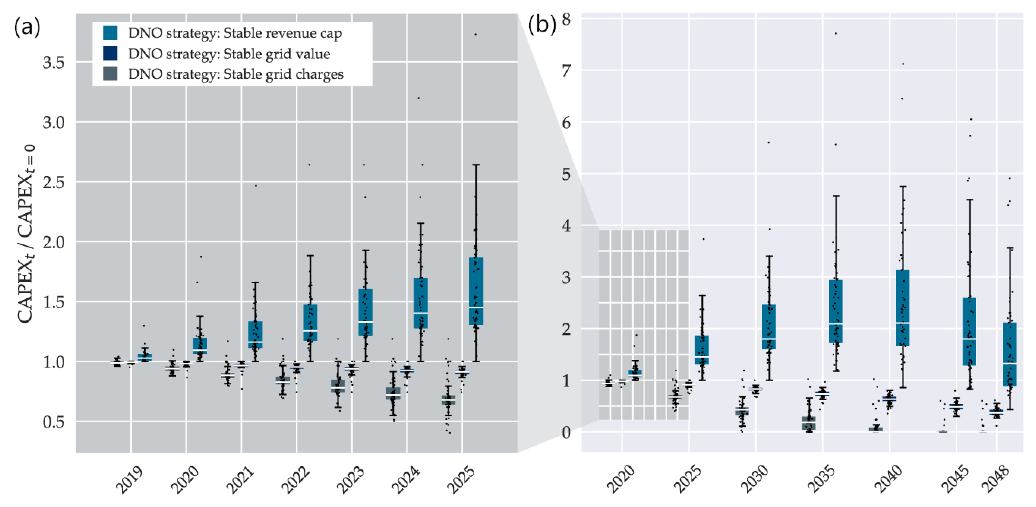
- “stable revenue cap”, an approach in which the DNO tries to keep the absolute revenue cap constant,
- “stable grid value”, an approach in which the revenue cap is constraint by a stable grid age, and
- “stable grid charges”, an approach in which the DNO tries to keep grid charges at a constant level.
2.5. Different Strategies for Grid Operation
3. Data and Methods
3.1. Gas Grid Data and Software Tools
3.2. Structural Network Analysis
3.2.1. Analysis of the Functional Relation between Grid Length and User Number
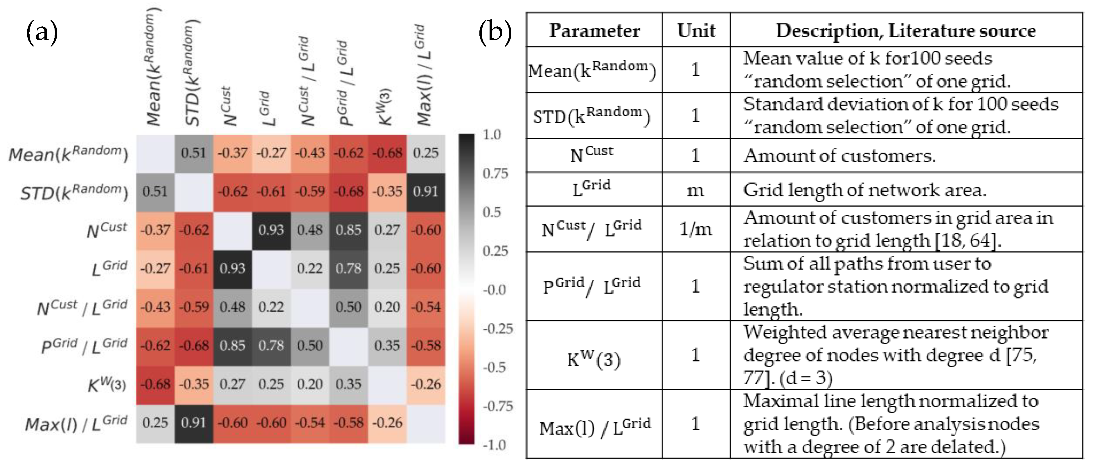
3.2.2. Correlation Analysis
3.3. Cash Flow Analysis
3.3.1. Economic Parameters and Principles
3.3.2. Optimization Model
- Only one renewal per line allowed within the planning horizon.
- Lines have to stay in operation as long as customers are connected [57].
- Lines have to be closed if no customer is connected anymore.
3.3.3. Simplified Cash Flow Calculation
- Stable grid charges: The grid charges are set to their initial value and is calculated, until its value reaches 0. After that, grid charges are a function of the yearly OPEX and supplied energy.
- Stable grid value: The mean rest book value factor is set to its initial value and the revenue cap is calculated.
- Stable revenue cap: The revenue cap is set to its initial value and the mean rest book value factor is calculated until its value reaches 1. After that, the revenue cap is a function of the yearly costs.
4. Results
4.1. Verification of Pressure Losses in the Distribution Grids
4.2. Structural Analysis
- k < 1: The decrease of grid length is slower than the decrease of customer number .
- k > 1: The decrease of grid length is faster than the decrease of customer number .
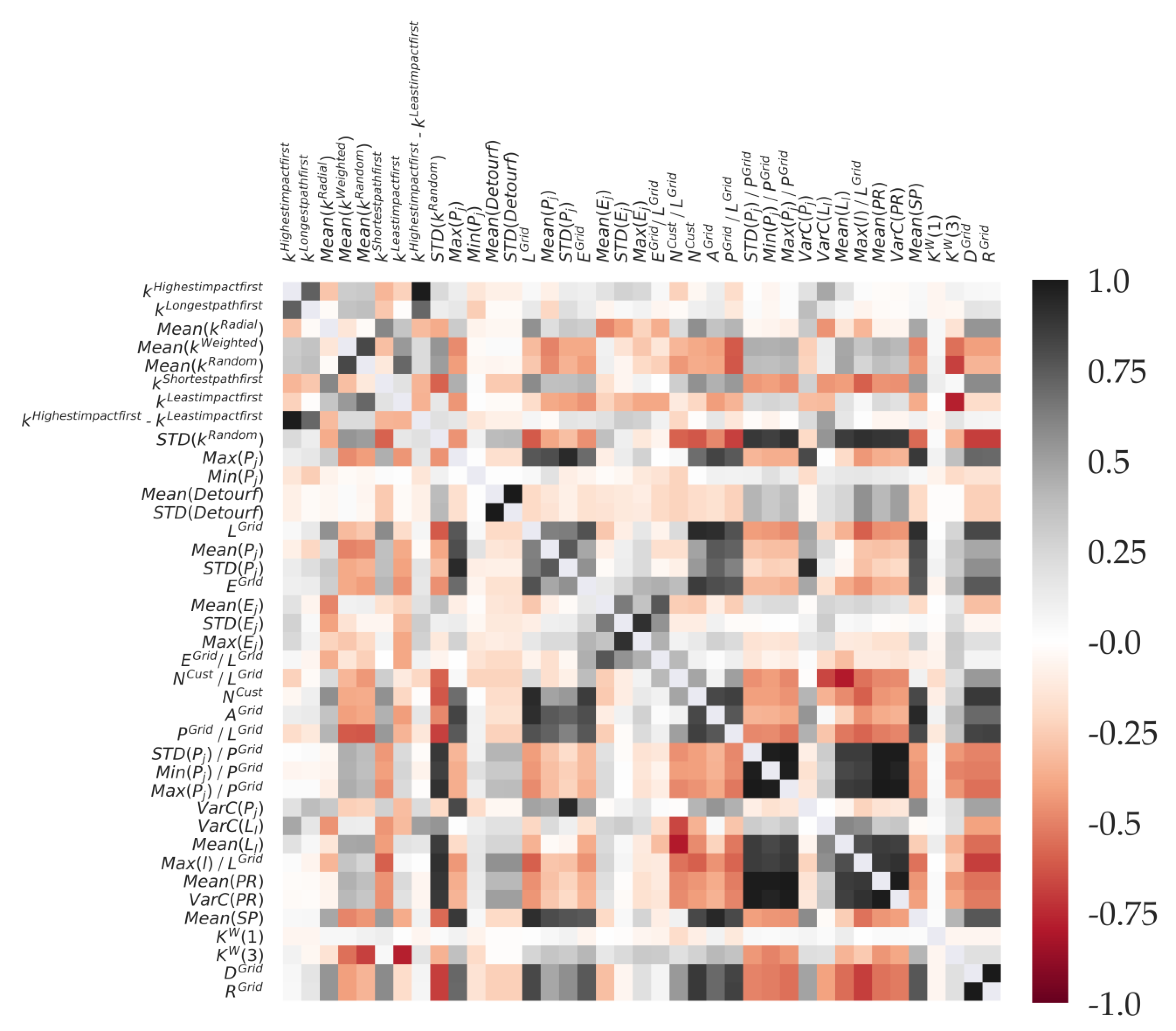
4.3. Correlation Analysis
4.4. Cost Analysis
4.4.1. DNO Costs of Operating a Natural Gas Infrastructure
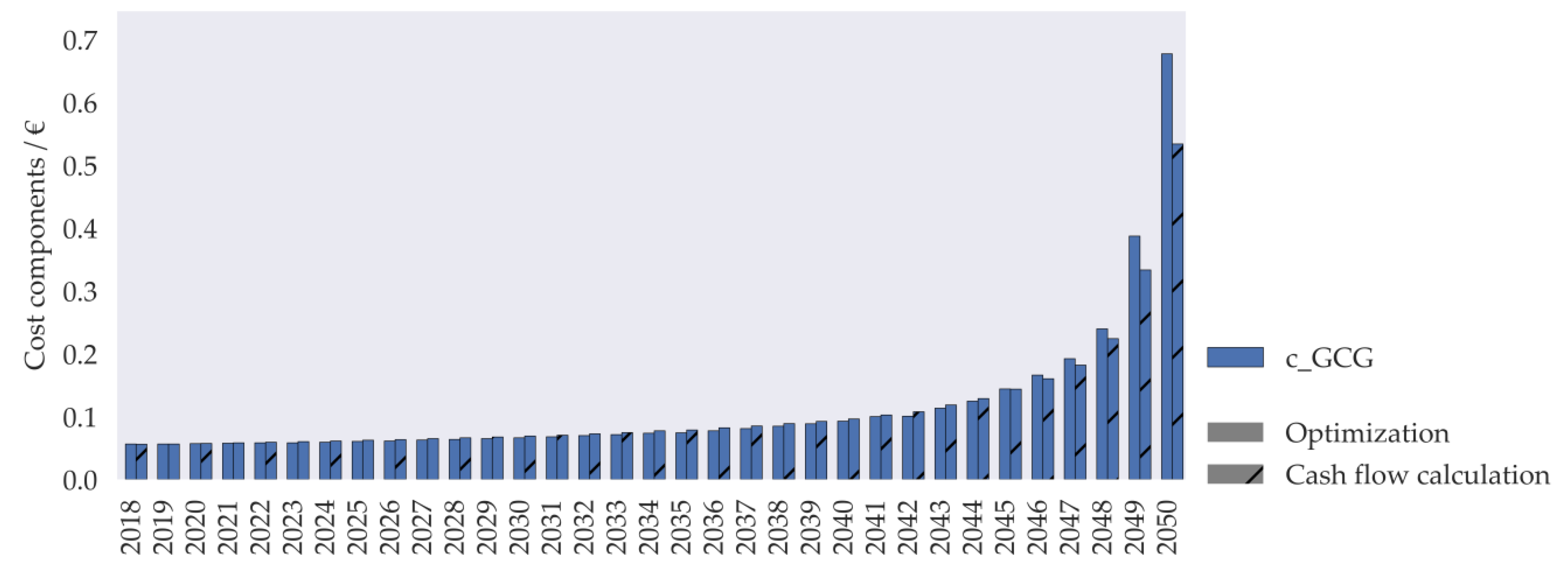
4.4.2. Comparison of Optimization-Based and Simplified Cash Flow Calculations
4.4.3. Cash Flow Analysis for All 57 Grid Areas
5. Discussion and Conclusions
5.1. Options, Risks and Conclusions for Distribution Network Operators
- Reducing the investment rate, and with that the CAPEX, leads to an increase of the grid age, thus its reliability drops, which in turn increases the operational costs.
- Shortening the depreciation period of lines has the same effects like a changed capitalization strategy in the long term.
5.2. Options, Risks and Conclusions for Grid Users
5.3. Macro-Economic Perspective and Regulatory Options
5.4. Further Research
5.4.1. Limits and Transferability of the Approach
5.4.2. Decisions of Single Actors
5.4.3. Interdependencies between the Decisions of Different Actors
Author Contributions
Funding
Acknowledgments
Conflicts of Interest
Appendix A. Nomenclature and Parametrization

| Name | Acronym | Name | Acronym |
|---|---|---|---|
| Building owner | BO | Grid charges | GC |
| Capital expenditure | CAPEX | Operational expenditure | OPEX |
| Distribution network operator | DNO | Revenue cap | RC |
| Domestic hot water | DHW | Space heating | SH |
| Parameter | Description [unit] | Value |
|---|---|---|
| Variables | ||
| Renewal of line ℓ in year 𝓇 (Binary decision variable of optimization model) | ||
| Closure of line ℓ in year 𝒸 (Binary decision variable of optimization model) | ||
| Grid charges gas in year 𝓉 [€/kWh] | ||
| Rest book value factor of line ℓ in year 𝓉 as a function of the binary decision variables | ||
| Mean rest book value factor of the whole grid in year 𝓉 | ||
| Age of line ℓ in year 𝓉 as a function of the binary decision variables [a] | ||
| Binary variable representing if a line is within its technical lifetime (function of the binary decision variables) | ||
| Power law function | ||
| Customer number of the grid | ||
| Cumulated line length of the grid [m] | ||
| k | Exponent of the power law function | |
| MSE | Mean squared error of power law fit | |
| R2 | Correlation coefficient of power law fit | |
| Cost components of the revenue cap | ||
| Capital expenditures [€] | ||
| Operational expenditures [€] | ||
| Calculated return on equity [€] | ||
| Interest on borrowed capital [€] | ||
| Calculated trade tax [€] | ||
| Calculated interest on borrowed capital [€] | ||
| Operational costs [€] | ||
| Loss costs [€] | ||
| Upstream grid charges [€] | ||
| Concession fees [€] | ||
| Parameters used in Section 2 (methods and materials) | ||
| Supplied energy in year 𝓉 [kWh/a] | Scenario specific | |
| Historical acquisition expenditures for line ℓ [€/m] | 214 * | |
| Line length of line ℓ [m] | Line specific | |
| Interest rate equity capital of line ℓ | 0.0691 * | |
| Amount of equity capital of line ℓ | 0.4 * | |
| Interest rate borrowed capital of line ℓ | 0.035 * | |
| Amount of borrowed capital of line ℓ | 0.6 * | |
| Trade tax rate | 0.1365 * | |
| Technical lifetime of a line [a] | 40 | |
| Planning horizon [a] | 33 | |
| Specific costs of upstream grid charges [€/kWh] | 0.01 | |
| Specific costs for concession fees [€/kWh] | 0.002 | |
| Specific lost costs [€/kWh] | 0.008 | |
| Loss factor | 0 | |
| Specific operational costs [€/m] | 10.71 | |
| Line age at the begin of planning horizon [a] | Line specific | |
| Length-weighted average age of the grid [a] | Grid specific | |
| Additional Parameters used in optimization model | ||
| Status matrix for renewal measure 𝓇 in year 𝓉 | See Appendix C.1 | |
| Status matrix for operation of line ℓ in year 𝓉 | See Appendix C.1 | |
| Status matrix for closure measure 𝒸 in year 𝓉 | See Appendix C.1 | |
| Energy demand of building 𝒿 in year 𝓉 [kWh] | Building and scenario specific | |
| Status matrix of line ℓ in year 𝓉 | Line and scenario specific | |
| Indices and sets | ||
| A building 𝒿 of all buildings connected to the grid | ||
| A line ℓ of all lines in the grid | ||
| A year 𝓉 within the planning horizon | ||
| Year of renewal measure 𝓇 of all possible years within the planning horizon | ||
| Year of closure measure 𝒸 of all possible years within the planning horizon | ||
Appendix B. Correlation Analysis
Appendix B.1. Parameters of Correlation Analysis
| Parameter | Unit | Description, Literature source |
|---|---|---|
| 1 | k value for “highest impact first” selection type of one grid. | |
| 1 | k value for “longest path first” selection type of one grid. | |
| 1 | Mean value of k for 100 seeds “radial random selection” of one grid. | |
| 1 | Mean value of k for 100 seeds “weighted random selection” of one grid. | |
| 1 | Mean value of k for 100 seeds “random selection” of one grid. | |
| 1 | k value for “Shortest path first” selection type of one grid. | |
| 1 | k value for “Least impact first” selection type of one grid. | |
| 1 | Difference of k values “highest impact first” and “least impact first” of one grid. | |
| 1 | Standard deviation of k for 100 seeds “random selection” of one grid. | |
| m | Longest path of a grid. | |
| m | Shortest path of a grid. | |
| 1 | Average value of the detour factor of a grid (detour factor: path length normalized with linear distance). | |
| 1 | Standard deviation of the detour factor of a grid. | |
| m | Grid length of a grid. | |
| m | Average value of all paths lengths of a grid. | |
| m | Standard deviation of all paths lengths of a grid. | |
| kWh/a | Cumulated yearly energy demand of a grid. | |
| kWh/a | Average energy demand of customers of a grid. | |
| kWh/a | Standard deviation of the customer’s energy demands in a grid. | |
| kWh/a | Maximal energy demand of a customer in a grid. | |
| kWh/(a * m) | Cumulated energy of grid area normalized to grid length. | |
| 1/(a * m) | Number of customers in grid area in relation to grid length. | |
| 1 | Number of customers in a grid area. | |
| m2 | Area size. | |
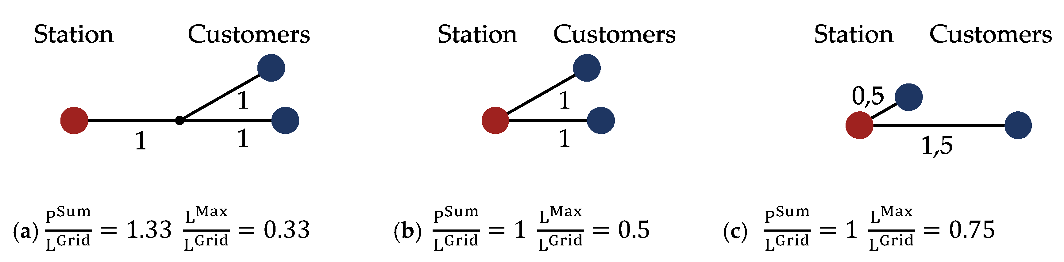
| 1 | Sum of all paths from user to regulator station normalized to grid length in a grid. | |
| 1 | Standard deviation of path lengths normalized to sum of path lengths in a grid. | |
| 1 | Shortest path normalized to sum of path lengths in a grid. | |
| 1 | Longest path normalized to sum of path lengths in a grid. | |
| 1 | Variation coefficient of path lengths in a grid. | |
| 1 | Variation coefficient of line lengths in a grid (of simplified graph, see chapt. 2). | |
| m | Average line length (of simplified graph, see chapt. 2). | |
| 1 | Maximal line length normalized to grid length (of simplified graph, see chapt. 2). | |
| 1 | Mean value of page rank [76,77]. (weights = line lengths; dumping factor d = 0.85) | |
| 1 | Variation coefficient of page rank. | |
| m | Sum of shortest paths between every nodes of the graph normalized by squared customers number (weights = line lengths) [91]. | |
| 1 | Weighted average nearest neighbor degree of nodes with degree d [75,77]. (d = 1) | |
| 1 | Weighted average nearest neighbor degree of nodes with degree d. (d = 3) | |
| 1 | Diameter of the graph, which represents its maximum eccentricity. The eccentricity of a node v is the maximum distance from v to all other nodes in G [92]. | |
| 1 | Radius of the graph, which represents its minimum eccentricity [92]. |
Appendix B.2. Correlation Matrix of All Parameters

Appendix B.3. Structural Parameters of the 57 Grid Areas
| Grid | Length/m | Number of Customers | Yearly Energy Demand/MWh | Length Weighted Average Initial Age/a |
|---|---|---|---|---|
| 0 | 480 | 4 | 233 | 15.1 |
| 1 | 2270 | 40 | 2235 | 33.1 |
| 2 | 2390 | 79 | 2224 | 28.3 |
| 3 | 1140 | 22 | 2496 | 36.1 |
| 4 | 2620 | 82 | 4529 | 31.4 |
| 5 | 4220 | 90 | 1581 | 22.4 |
| 6 | 7680 | 266 | 6787 | 35.8 |
| 7 | 4460 | 124 | 8828 | 20.7 |
| 8 | 8630 | 299 | 8032 | 34.6 |
| 9 | 5590 | 174 | 4877 | 25.7 |
| 10 | 650 | 17 | 2335 | 29.0 |
| 11 | 5200 | 191 | 5445 | 27.1 |
| 12 | 3660 | 69 | 3625 | 22.9 |
| 13 | 8080 | 229 | 6524 | 24.5 |
| 14 | 1830 | 44 | 1575 | 29.9 |
| 15 | 2430 | 75 | 7457 | 29.1 |
| 16 | 5510 | 166 | 2284 | 20.4 |
| 17 | 4590 | 189 | 3889 | 28.6 |
| 18 | 3210 | 148 | 1638 | 17.0 |
| 19 | 4270 | 167 | 5633 | 22.7 |
| 20 | 2870 | 126 | 3009 | 29.1 |
| 21 | 980 | 31 | 1444 | 28.7 |
| 22 | 5650 | 212 | 4550 | 25.1 |
| 23 | 3620 | 127 | 4540 | 30.7 |
| 24 | 1510 | 61 | 2708 | 26.1 |
| 25 | 2150 | 36 | 2185 | 16.9 |
| 26 | 6390 | 152 | 5660 | 21.6 |
| 27 | 9510 | 247 | 7060 | 26.4 |
| 28 | 5890 | 209 | 4286 | 26.2 |
| 29 | 2990 | 64 | 4046 | 22.0 |
| 30 | 4440 | 205 | 5229 | 33.6 |
| 31 | 2550 | 130 | 2690 | 35.9 |
| 32 | 5650 | 228 | 7193 | 25.5 |
| 33 | 5140 | 234 | 8473 | 30.9 |
| 34 | 7680 | 245 | 9616 | 23.4 |
| 35 | 4660 | 199 | 9029 | 29.2 |
| 36 | 7520 | 363 | 19,092 | 29.9 |
| 37 | 5070 | 180 | 13,916 | 30.8 |
| 38 | 500 | 8 | 136 | 14.3 |
| 39 | 3810 | 129 | 3322 | 21.3 |
| 40 | 8110 | 258 | 13,229 | 31.3 |
| 41 | 7300 | 227 | 6336 | 35.1 |
| 42 | 10,080 | 390 | 16,786 | 27.2 |
| 43 | 4200 | 131 | 4694 | 27.0 |
| 44 | 4960 | 181 | 4626 | 21.4 |
| 45 | 3030 | 100 | 2583 | 28.6 |
| 46 | 2390 | 76 | 2133 | 26.3 |
| 47 | 6940 | 281 | 14,294 | 28.9 |
| 48 | 1600 | 101 | 3822 | 33.0 |
| 49 | 3290 | 193 | 8625 | 32.1 |
| 50 | 470 | 23 | 1538 | 35.8 |
| 51 | 6300 | 276 | 17,462 | 28.7 |
| 52 | 5550 | 144 | 8993 | 29.5 |
| 53 | 2790 | 56 | 4012 | 19.5 |
| 54 | 10,760 | 481 | 20,192 | 31.5 |
| 55 | 11,960 | 507 | 21,045 | 33.3 |
| 56 | 1350 | 31 | 1024 | 21.5 |
Appendix C. Cash Flow Analysis
Appendix C.1 Optimization Model
Appendix C.2. Simplified Cash Flow Model
Appendix C.3. Global Scenario of the Cost Analysis

Appendix C.4. Results of the Cost Analysis

References
- Renewable Energy Policy Network for the 21st Century (REN21). Renewables 2018—Global Status Report; Renewable Energy Policy Network for the 21st Century (REN21): Paris, France, 2018. [Google Scholar]
- U.S. Energy Information Administration. International Energy Outlook 2019; U.S. Energy Information Administration: Washington, DC, USA, 2019.
- Global Energy Assessment Writing Team. Global Energy Assessment (GEA); Cambridge University Press: Cambridge, UK; New York, NY, USA; Melbourne, Australia, 2012; ISBN 9781107005198. [Google Scholar]
- Eurostat. Final Energy Consumption in Households. 2018. Available online: https://https://www.ec.europa.eu/eurostat/cache/metadata/EN/t2020_rk200_esmsip2.htm (accessed on 9 December 2019).
- Honoré, A. Decarbonisation of Heat in Europe: Implications for Natural Gas Demand; Oxford Institute for Energy Studies: Oxford, UK, 2018. [Google Scholar]
- Hecking, H.; Hintermayer, M.; Lencz, D.; Wagner, J. Energiemarkt 2030 und 2050—Der Beitrag von Gas-und Wärmeinfrastruktur zu Einer Effizienten CO2-Minderung; ewi Energy Research & Scenarios: Cologne, Germany, 2017. [Google Scholar]
- Bothe, D.; Janssen, M.; van der Poel, S.; Eich, T.; Bongers, T.; Kellermann, J.; Lück, L.; Chan, H.; Ahlert, M.; Borrás, C.A.B.; et al. Der Wert der Gasinfrastruktur für die Energiewende in Deutschland—Eine modellbasierte Analyse—Eine Studie im Auftrag der Vereinigung der Fernleitungsnetzbetreiber (FNB Gas e.V.); Frontier Eonomics: London, UK; Institut für Elektrische Anlagen und Energiewirtschaft (IAEW): Aachen, Germany; 4Management: Düsseldorf, Germany; EMCEL: Köln, Germany, 2017. [Google Scholar]
- Henning, H.M.; Palzer, A. Energiesystem Deutschland 2050; Fraunhofer-Institut für Solare Energiesysteme (ISE): Freiburg, Germany, 2013. [Google Scholar]
- Deutsch, M.; Gerhardt, N.; Sandau, F.; Becker, S.; Scholz, A.; Schumacher, P.; Schmidt, D. Wärmewende 2030—Schlüsseltechnologien zur Erreichung der mittel-und Langfristigen Klimaschutzziele im Gebäudesektor—Eine Studie im Auftrag der Agora Energiewende; Fraunhofer-Institut für Windenergie und Energiesystemtechnik (IWES): Bremerhaven, Germany; Fraunhofer-Institut für Bauphysik (IBP): Stuttgart, Germany, 2017. [Google Scholar]
- Fernleitungsnetzbetreiber Gas (FNB Gas). Prognos, Szenariorahmen für den Netzentwicklungsplan Gas 2018–2028 der Fernleitungsnetzbetreiber—Eine Studie im Auftrag der Deutschen; Fernleitungsnetzbetreiber (FNB): Berlin, Germany, 2017. [Google Scholar]
- Ziesing, H.J.; Repenning, J.; Emele, L.; Blanck, R.; Böttcher, H.; Dehoust, G.; Förster, H.; Greiner, B.; Harthan, R.; Henneberg, K.; et al. Klimaschutzszenario 2050—2. Endbericht—Eine Studie im Auftrag des Bundesministeriums für Umwelt, Naturschutz, Bau und Reaktorsicherheit; Fraunhofer-Institut für System-und Innovationsforschung: Karlsruhe, Germany, 2015. [Google Scholar]
- Mastorakos, S.; Madrigal, J.; Duffy, E.; Ebertin, M.; Bosso, E. The Future of Natural Gas in the United States; United States Ecologic Institute: Washington, DC, USA, 2017. [Google Scholar]
- Feijoo, F.; Iyer, G.C.; Avraam, C.; Siddiqui, S.A.; Clarke, L.E.; Sankaranarayanan, S.; Binsted, M.T.; Patel, P.L.; Prates, N.C.; Torres-Alfaro, E.; et al. The future of natural gas infrastructure development in the United states. Appl. Energy 2018, 228, 149–166. [Google Scholar] [CrossRef]
- Costello, K.W. Why natural gas has an uncertain future. Electr. J. 2017, 30, 18–22. [Google Scholar] [CrossRef]
- Mac Kinnon, M.A.; Brouwer, J.; Samuelsen, S. The role of natural gas and its infrastructure in mitigating greenhouse gas emissions, improving regional air quality, and renewable resource integration. Prog. Energy Combus. Sci. 2018, 64, 62–92. [Google Scholar] [CrossRef]
- Jianhong, Y. Analysis of sustainable development of natural gas market in China. Nat. Gas Ind. B 2018, 5, 644–651. [Google Scholar] [CrossRef]
- Ailin, J. Progress and prospects of natural gas development technologies in China. Nat. Gas Ind. B 2018, 5, 547–557. [Google Scholar] [CrossRef]
- Däuper, O.; Strasser, T.; Lange, H.; Tischmacher, D.; Fimpel, A.; Kaspers, J.; Koulaxidis, S.; Warg, F.; Baudisch, K.; Bergmann, P.; et al. Wärmewendestudie—Die Wärmewende und ihre Auswirkungen auf die Gasverteilnetze; Becker Büttner Held: München, Deutschland, 2018. [Google Scholar]
- Hickey, C.; Deane, P.; McInerney, C.; Gallachóir, B.Ó. Is there a future for the gas network in a low carbon energy system? Energy Policy 2019, 126, 480–493. [Google Scholar] [CrossRef]
- Speirs, J.; Balcombe, P.; Johnson, E.; Martin, J.; Brandon, N.; Hawkes, A. A greener gas grid: What are the options. Energy Policy 2018, 118, 291–297. [Google Scholar] [CrossRef]
- Qadrdan, M.; Fazeli, R.; Jenkins, N.; Strbac, G.; Sansorn, R. Gas and electricity supply implications of decarbonising heat sector in GB. Energy 2019, 169, 50–60. [Google Scholar] [CrossRef]
- McGlade, C.; Pye, S.; Ekins, P.; Bradshadw, M.; Watson, J. The future role of natural gas in the UK: A bridge to nowhere? Energy Policy 2018, 113, 454–465. [Google Scholar] [CrossRef]
- Schlesinger, M.; Hofer, P.; Kemmler, A.; Kirchner, A.; Koziel, S.; Ley, A.; Piégsa, A.; Seefeldt, F.; Straßburg, S.; Weinert, K.; et al. Entwicklung der Energiemärkte—Energiereferenzprognose—Projekt Nr. 57/12 Studie im Auftrag des Bundesministeriums für Wirtschaft und Technologie—Eine Studie im Auftrag des Bundesministeriums für Wirtschaft und Technologie; Energiewirtschaftliches Institut an der Universität zu Köln (EWI): Köln, Germany; Gesellschaft für Wirtschaftliche Strukturforschung mbH (GWS): Osnabrück, Germany; Prognos: Basel, Switzerland, 2014. [Google Scholar]
- Gerbert, P.; Herhold, P.; Burchardt, J.; Schönberger, S.; Rechenmaher, F.; Kirchner, A.; Kemmler, A.; Wünsch, M. Klimapfade für Deutschland—Eine Studie im Auftrag des Bundesverbandes der Deutschen Industrie e.V. (BDI); The Boston Consulting Group: Boston, MA, USA; Prognos: Basel, Switzerland, 2018. [Google Scholar]
- Gerhardt, N.; Sandau, F.; Scholz, A.; Hahn, H.; Schumacher, P.; Sager, C.; Bergk, F.; Kämper, C.; Knörr, W.; Kräck, J.; et al. Interaktion EE-Strom, Wärme und Verkehr—Analyse der Interaktion zwischen den Sektoren Strom, Wärme/Kälte und Verkehr in Deutschland in Hinblick auf steigende Anteile fluktuierender Erneuerbarer Energien im Strombereich unter Berücksichtigung der europäischen Entwicklung—Ableitung von optimalen strukturellen Entwiklungspfaden für den Verkehrs-und Wärmesektor; Fraunhofer-Institut für Windenergie und Energiesystemtechnik IWES: Bremerhaven, Germany; Fraunhofer-Institut für Bauphysik IBP: Stuttgart, Germany; Institut für Energie-und Umweltforschung IFEU: Heidelberg, Germany; Stiftung Umweltenergierecht: Würzburg, Germany, 2015. [Google Scholar]
- Enervis Energy Advisors GmbH. Klimaschutz durch Sektorenkopplung: Optionen, Szenarien, Kosten; Enervis Energy Advisors GmbH: Berlin, Germany, 2017. [Google Scholar]
- Nitsch, J. SZEN-15—Aktuelle Szenarien der Deutschen Energieversorgung unter Berücksichtigung der Eckdaten des Jahres 2014; Bundesverband Erneuerbare Energien e.V.: Berlin, Germany, 2015. [Google Scholar]
- Nitsch, J. SZEN-17—Erfolgreiche Energiewende nur mit Verbesserter Energieeffizienz—Aktuelle Szenarien 2017 der Deutschen Energieversorgungund einem Klimagerechten Energiemarkt; Bundesverband Erneuerbare Energien e.V.: Berlin, Germany, 2017. [Google Scholar]
- Klein, S.; Klein, S.W.; Steinert, T.; Fricke, A.; Peschel, D. Erneuerbare Gase—Ein Systemupdate der Energiewende; Eine Studie im Auftrag von der Initiative Erdgasspeicher; Bundesverband WindEnergie: Berlin, Germany; Enervis energy advisors GmbH: Berlin, Germany, 2017. [Google Scholar]
- Zukunft ERDGAS e.V. Wärmemarkt 2050—So Erreicht Deutschland Kosteneffizient das Klimaziel; Zukunft ERDGAS e.V.: Berlin, Germany, 2017. [Google Scholar]
- BMU, Arbeitsgruppe IK III 1. Klimaschutzplan 2050—Klimapolitische Grundsätze und Ziele der Bundesregierung; Bundesministerium für Umwelt, Naturschutz und Nukleare Sicherheit (BMU): Berlin, Germany, 2019. [Google Scholar]
- Wittke, F. Auswertungstabellen zur Energiebilanz Deutschland—1990 bis 2017; Arbeitsgemeinschaft Energiebilanzen e.V. AGEB: Berlin, Germany, 2018. [Google Scholar]
- FNB Gas; Prognos. Szenariorahmen für den Netzentwicklungsplan Gas 2018-2028 der Fernleitungsnetzbetreiber—Konsultationsdokument; Eine Studie im Auftrag; Fernleitungsnetzbetreiber: Berlin, Germany, 2017. [Google Scholar]
- Nymoen, H.; Siebert, K.; Niemann, E. Sanierungsfahrpläne für den Wärmemarkt: Wie Können sich Private Hauseigentümer die Energiewende Leisten? Eine Studie im Auftrag; Zukunft ERDGAS e.V.: Berlin, Germany; Nymoen Strategieberatung: Berlin, Germany, 2014. [Google Scholar]
- Evins, R. A review of computational optimisation methods applied to sustainable building design. Renew. Sustain. Energy Rev. 2013, 22, 230–245. [Google Scholar] [CrossRef]
- Machairas, V.; Tsangrassoulis, A.; Axarli, K. Algorithms for optimization of building design: A review. Renew. Sustain. Energy Rev. 2014, 31, 101–112. [Google Scholar] [CrossRef]
- Huang, Y.; Niu, J.-L. Optimal building envelope design based on simulated performance: History, current status and new potentials. Energy Build. 2016, 117, 387–398. [Google Scholar] [CrossRef]
- Ansorge, K.; Streblow, R. Genetischer Algorithmus zur Kombinatorischen Optimierung von Gebäudehülle und Anlagentechnik—Optimale Sanierungspakete für Ein-und Zweifamilienhäuser; Gebäude-Energiewende Arbeitspapier 7: Berlin, Germany, 2017. [Google Scholar]
- Appen, J.V.; Braun, M. Strategic decision making of distribution network operators and investors in residential photovoltaic battery storage systems. Appl. Energy 2018, 230, 540–550. [Google Scholar] [CrossRef]
- Huke, L. Energetische Optimierung der Öffentlichen Gasversorgung—Dissertation. Ph.D. Thesis, Technische Universität Bergakademie Freiberg, Freiberg, Germany, 2002. [Google Scholar]
- Sanft, S. Modell zur Wirtschaftlichkeitsbewertung von Instandhaltungsstrategien bei Gasverteilnetzen im regulierten deutschen Gasmarkt—Dissertation. Ph.D. Thesis, Ruhr-Universität Bochum, Bochum, Germany, 2015. [Google Scholar]
- Hübner, M.; Haubrich, H.-J. Long-Term Pressure-Stage Comprehensive Planning of Natural Gas Networks in Handbook of Networks in Power Systems II; Sorokin, A., Rebennack, S., Pardalos, P., Iliadis, N.A., Pereira, M.V.F., Eds.; Springer: Berlin, Germany, 2012; pp. 37–59. ISBN 978-3-642-44612-2. [Google Scholar]
- Zeng, Q.; Zhang, B.; Fang, J.; Chen, Z. A bi-level programming for multistage co-expansion planning of the integrated gas and electricity system. Appl. Energy 2017, 200, 192–203. [Google Scholar] [CrossRef]
- Unishuay-Vila, C.; Marangon-Lima, J.W.; Zambroni de Souza, A.C.; Perez-Arriaga, I.J.; Balestrassi, P.P. A model to long-term, multiarea, multistage, and integrated expansion planning of electricity and natural gas systems. IEEE Trans. Power Syst. 2010, 25. [Google Scholar] [CrossRef]
- Chaudry, M.; Jenkins, N.; Qadrdan, M.; Wu, J. Combined gas and electricity network expansion planning. Appl. Energy. 2014, 113, 1171–1187. [Google Scholar] [CrossRef]
- Odetayo, B.; MacCormack, J.; Rosehart, W.D.; Zareipour, H.; Seifi, A.R. Integrated planning of natural gas and electric power systems. Electr. Power Energy Syst. 2018, 103, 593–602. [Google Scholar] [CrossRef]
- Qiu, J.; Yang, Z.; Hua, J.; Meng, K.; Zheng, Y.; Hill, D.J. Low carbon oriented expansion planning of integrated gas and power systems. IEEE Trans. Power Syst. 2015, 30, 1035–1046. [Google Scholar] [CrossRef]
- Saldarriaga, C.A.; Hincapié, R.A.; Salazar, H. An integrated expansion planning model of electric and natural gas distribution systems considering demand uncertainty. In Proceedings of the 2015 IEEE Power & Energy Society General Meeting, Denver, CO, USA, 26–30 July 2015. [Google Scholar] [CrossRef]
- Odetayo, B.; MacCormack, J.; Rosehart, W.D.; Zareipour, H. Integrated planning of natural gas and electricity distribution networks with the presence of distributed natural gas fired generators. In Proceedings of the 2016 IEEE Power and Energy Society General Meeting, Boston, MA, USA, 17–21 July 2016. [Google Scholar] [CrossRef]
- Bakken, B.H.; Mindeberg, S.K. Linear models for optimization of interconnected gas and electricity networks. In Proceedings of the 2009 IEEE Power & Energy Society General Meeting, Calgary, AB, Canada, 26–30 July 2009. [Google Scholar] [CrossRef]
- Zeng, Q.; Fang, J.; Li, J.; Chen, Z. Steady-State analysis of the integrated natural gas and electric power system with bi-directional energy conversion. Appl. Energy. 2016, 184, 1483–1492. [Google Scholar] [CrossRef]
- Wang, I.E.; Clandinin, T.R. The influence of wiring economy on nervous system evolution. Curr. Biol. 2016, 26, 1101–1108. [Google Scholar] [CrossRef]
- Watts, D.J.; Strogatz, S.H. Collective dynamics of ‘small-world’ networks. Nature 1998, 393, 440–442. [Google Scholar] [CrossRef] [PubMed]
- Braunstein, L.A.; Cohen, R.; Buldyrev, S.V.; Havlin, S. Optimal paths in disordered complex networks. Phys. Rev. Lett. 2003, 91. [Google Scholar] [CrossRef] [PubMed]
- Wen, Q.; Stepanyants, A.; Elston, G.N.; Grosberg, A.Y.; Chklovskii, D.B. Maximization of the connectivity repertoire as a statistical principle governing the shapes of dendritic arbors. Proc. Natl. Acad. Sci. USA 2009, 106, 12536–12541. [Google Scholar] [CrossRef] [PubMed]
- Peng, D.; Poudineh, R. A holistic framework for the study of interdependence between electricity and gas sectors. Energy Strategy Rev. 2016, 13–14, 32–52. [Google Scholar] [CrossRef]
- Bundesministerium der Justiz und Verbraucherschutz. Gesetz über die Elektrizitäts-und Gasversorgung (Energiewirtschaftsgesetz-EnWG); Energiewirtschaftsgesetz 7 July 2005; Bundesministerium der Justiz und Verbraucherschutz: Berlin, Germany, 2005.
- Christensen, L.R.; Greene, W.H. Economies of scale in U.S. electric power generation. J. Political Econ. 1976, 84, 655–676. [Google Scholar] [CrossRef]
- Erdmann, G.; Zweifel, P. Energieökonomik, 2nd ed.; Springer: Berlin/Heidelberg, Germany, 2010; ISBN 978-3-642-12777-9. [Google Scholar]
- Cambini, C.; Meletiou, A.; Bompard, E.; Masera, M. Market and regulatory factors influencing smart-grid investment in Europe: Evidence from pilot projects and implications for reform. Util. Policy 2016, 40, 36–47. [Google Scholar] [CrossRef]
- Andra, B. CEER Report: Report on Regulatory Frameworks for European Energy Networks; Council of European Energy Regulators: Brussels, Belgium, 2019. [Google Scholar]
- Diekmann, J.; Leprich, U.; Ziesing, H.-J. Regulierung der Stromnetze in Deutschland; Hans-Böckler-Stiftung: Düsseldorf, Germany, 2007; ISBN 978-3-86593-067-5. [Google Scholar]
- Bundesministerium der Justiz und Verbraucherschutz. Verordnung über die Anreizregulierung der Energieversorgungsnetze (Anreizregulierungsverordnung-ARegV); Anreizregulierungsverordnung vom 29 Oktober 2007; Bundesministerium der Justiz und Verbraucherschutz: Berlin, Germany, 2007.
- Agrell, P.; Bogetoft, P.; Koller, M.; Trinkner, U. Effizienzvergleich für Verteilernetzbetreiber Strom 2013—Ergebnisdokumentation und Schlussbericht; Swiss Economics: Zürich, Switzerland; SUMICSID: Stånga, Sweden, 2014. [Google Scholar]
- Bundesnetzagentur; Bundeskartellamt. Monitoringbericht 2018; Bundesnetzagentur: Bonn, Germany; Bundeskartellamt: Bonn, Germany, 2019.
- OpenStreetMap Contributors. 2019. Available online: https://wiki.openstreetmap.org/wiki/Researcher_Information (accessed on 10 December 2019).
- Fischer-Uhrig, I. STANET Netzberechnung—Für Gas, Wasser, Strom, Fernwärme und Abwasser. 2020. Available online: www.stafu.de/de/home.html (accessed on 9 January 2020).
- Hart, W.E.; Laird, C.D.; Watson, J.-P.; Woodruff, D.L.; Hackebeil, G.A.; Nicholson, B.L.; Siirola, J.D. Pyomo—Optimization Modeling in Python, 2nd ed.; Springer: Cham, Switzerland, 2017; ISBN 978-3-319-58821-2. [Google Scholar]
- Hart, W.E.; Watson, J.-P.; Woodruff, D.L. Pyomo: Modeling and solving mathematical programs in Python. Math. Program. Comput. 2011, 3, 219–260. [Google Scholar] [CrossRef]
- Hagberg, A.A.; Schult, D.A.; Swart, P.J. Exploring network structure, dynamics, and function using NetworkX. In Proceedings of the 7th Python in Science Conference (SciPy 2008), Pasadena, CA, USA, 19–24 August 2008; pp. 11–15. [Google Scholar]
- Pedregosa, F.; Varoquaux, G.; Gramfort, A.; Michel, V.; Thirion, B.; Grisel, O.; Blondel, M.; Prettenhofer, P.; Weiss, R.; Dubourg, V.; et al. Scikit-Learn: Machine learning in Python. J. Mach. Learn. Res. 2012, 12, 2825–2830. [Google Scholar]
- IBM. IBM ILOG CPLEX Optimization Studio. 2020. Available online: https://www.ibm.com/products/ilog-cplex-optimization-studio (accessed on 9 January 2020).
- Rival, I. Algorithms and Order, 1st ed.; Kluwer Academic Publishers: Dordrecht, The Netherlands, 1989; ISBN 978-94-010-7691-3. [Google Scholar]
- The SciPy Community. SciPy Documentation—Scipy.optimize.curve_fit. 2019. Available online: https://www.docs.scipy.org/doc/scipy/reference/generated/scipy.optimize.curve_fit.html (accessed on 9 December 2019).
- Barrat, A.; Barthélemy, M.; Pastor-Satorras, R.; Vespignani, A. The architecture of complex weighted networks. Proc. Natl. Acad. Sci. USA 2004, 101, 3747–3752. [Google Scholar] [CrossRef]
- Langville, A.N.; Meyer, C.D. A survey of eigenvector methods of web information retrieval. Soc. Ind. Appl. Math. Rev. 2005, 47, 135–161. [Google Scholar] [CrossRef]
- NetworkX Developers. NetworkX Documentation Reference. 2015. Available online: https://networkx.github.io/documentation/networkx-1.10/reference/index.html (accessed on 9 December 2019).
- Cerbe, G.; Lendt, B. Grundlagen der Gastechnik-Gasbeschaffung-Gasverteilung-Gasverwendung, 8th ed.; Brüggemann, K., Dehli, M., Gröschl, F., Heikrodt, K., Kleiber, T., Kuck, J., Mischner, J., Schmidt, T., Seemann, A., Thielen, W., Eds.; Carl Hanser Verlag: Munich, Germany, 2016; ISBN 978-3-446-44965-7. [Google Scholar]
- Bundesministerium der Justiz und Verbraucherschutz. Verordnung über die Vergabe von Konzessionen (Konzessionsvergabeverordnung—KonzVgV); Konzessionsvergabeverordnung vom 12 April 2016; Bundesministerium der Justiz und Verbraucherschutz: Berlin, Germany, 2016.
- Lee, C.W.; Ng, S.K.K.; Zhong, J. 2nd Broadband Convergence Networks BcN 2007. In Proceedings of the 2nd IEEE/IFIP International Workshop on Broadband Convergence Networks, 2007 (BcN ′07), Munich, Germany, 21 May 2007; IEEE: Piscataway, NJ, USA, 2007. [Google Scholar]
- Molina, J.D.; Contreras, J.; Rudnick, H. A risk-constrained project portfolio in centralized transmission expansion planning. IEEE Syst. J. 2017, 11, 1653–1661. [Google Scholar] [CrossRef]
- Zhang, Y.; Wang, X.; Zhang, W.; Wu, Z.; Zhang, Z.; Qiang, C. Co-Planning of generation and transmission capacity based on portfolio theory. In Proceedings of the 2016 IEEE PES Asia-Pacific Power and Energy Engineering Conference (APPEEC), Xi’an, China, 25–28 October 2016. [Google Scholar]
- Schachter, J.A.; Mancarella, P. A critical review of Real Options thinking for valuing investment flexibility in Smart Grids and low carbon energy systems. Renew. Sustain. Energy Rev. 2016, 56, 261–271. [Google Scholar] [CrossRef]
- Odetayo, B.; MacCormack, J.; Rosehart, W.D.; Zareipour, H. A real option assessment of flexibilities in the integrated planning of natural gas distribution network and distributed natural gas-fired power generations. Energy 2018, 143, 257–272. [Google Scholar] [CrossRef]
- Ansorge, K.; Streblow, R. Gebäudesteckbriefe—Exemplarische Sanierungsstrategien für Wohngebäude am Beispiel von ausgewählten Prototypgebäuden; Gebäude-Energiewende Arbeitspapier 8: Berlin, Germany, 2017. [Google Scholar]
- Stieß, I.; van der Land, V.; Birzle-Harder, B.; Deffner, J. Handlungsmotive-hemmnisse und Zielgruppen für eine Energetische Gebäudesanierung—Ergebnisse einer Standardisierten Befragung von Eigenheimsanierern; Institut für Ökologische Wirtschaftsforschung IÖW: Berlin, Germany, 2010. [Google Scholar]
- Renz, I.; Hacke, U. Einflussfaktoren auf die Sanierung im Deutschen Wohngebäudebestand—Ergebnisse einer Qualitativen Studie zu Sanierungsanreizen und-Hemmnissen priater und intitutioneller Eigentümer—Eine Untersuchung im Auftrag der KfW Bankengruppe; Institut Wohnen und Umwelt IWU: Darmstadt, Germany, 2016. [Google Scholar]
- Hundt, M. Investitionsplanung Unter Unsicheren Einflussgrößen; Springer Fachmedien Wiesbaden: Wiesbaden, Germany, 2015. [Google Scholar]
- Khalilpour, R.; Vassallo, A. Leaving the grid: An. ambition or a real choice? Energy Policy 2015, 82, 207–221. [Google Scholar] [CrossRef]
- Laws, N.D.; Epps, B.P.; Peterson, S.O.; Laser, M.S.; Wanjiru, G.K. On the utility death spiral and the impact of utility rate structures on the adoption of residential solar photovoltaics and energy storage. Appl. Energy 2017, 185, 627–641. [Google Scholar] [CrossRef]
- NetworkX Developers. NetworkX Documentation—Algorithms—Average_Shortest_Path_Length. 2015. Available online: https://networkx.github.io/documentation/networkx-1.10/reference/generated/networkx.algorithms.shortest_paths.generic.average_shortest_path_length.html (accessed on 11 December 2019).
- NetworkX Developers. NetworkX Documentation—Algorithms—Distance Measures. 2015. Available online: https://networkx.github.io/documentation/networkx-1.10/reference/algorithms.distance_measures.html (accessed on 11 December 2019).
- Bisschop, J. AIMMS Optimization Modeling; AIMMS B.V.: Haarlem, The Netherlands, 2019. [Google Scholar]


| Country | Gas DNO | |
|---|---|---|
| Regulation Method | Incentive Regulation | |
| Austria | Price-cap | Yes |
| France | Revenue-cap | Yes |
| Germany | Revenue-cap | Yes |
| Ireland | Revenue-cap | Yes |
| Norway | Revenue-cap | Yes |
| Netherlands | Price-cap | Yes |
| Cost Component | Grid Length | Grid Age | Energy | Overall Share in Case Study ** (%) | |
|---|---|---|---|---|---|
| CAPEX | Calc. return equity | + | − | 9.9 | |
| Calc. trade tax | + | − | 1.3 | ||
| Interests on borrowed capital | + | − | 6.6 | ||
| Calc. depreciations | + | − | 15.0 | ||
| OPEX | Operational costs | + | * | * | 33.6 |
| Loss costs | + | 0.0 | |||
| Upstream grid charges | + | 19.0 | |||
| Concession fees | + | 14.7 |
| Name | Selection Type; Seeds | Determination of Customer Exits | Interpretation |
|---|---|---|---|
| Shortest path first | Ranked selection; 1 | Order and drop customers by their path length to the connection point. | Worst case |
| Longest path first | Best case | ||
| Least impact first | Drop costumers by their impact on grid length. Determine the impact after every exit. | Worst case | |
| Highest impact first | Best case | ||
| Random selection | Stochastic selection; 100 | Choose customers for exit randomly. | Stochastic selection |
| Weighted random selection | Choose customer exits based on a conditional probability calculated by building ages and pseudo random numbers. | Stochastic selection based on building age | |
| Radial selection | Choose a random starting point. Drop customers by radial distance to this point. Start with the lowest distance. | Extreme case of a weighted stochastic selection |
© 2020 by the authors. Licensee MDPI, Basel, Switzerland. This article is an open access article distributed under the terms and conditions of the Creative Commons Attribution (CC BY) license (http://creativecommons.org/licenses/by/4.0/).
Share and Cite
Then, D.; Spalthoff, C.; Bauer, J.; Kneiske, T.M.; Braun, M. Impact of Natural Gas Distribution Network Structure and Operator Strategies on Grid Economy in Face of Decreasing Demand. Energies 2020, 13, 664. https://doi.org/10.3390/en13030664
Then D, Spalthoff C, Bauer J, Kneiske TM, Braun M. Impact of Natural Gas Distribution Network Structure and Operator Strategies on Grid Economy in Face of Decreasing Demand. Energies. 2020; 13(3):664. https://doi.org/10.3390/en13030664
Chicago/Turabian StyleThen, Daniel, Christian Spalthoff, Johannes Bauer, Tanja M. Kneiske, and Martin Braun. 2020. "Impact of Natural Gas Distribution Network Structure and Operator Strategies on Grid Economy in Face of Decreasing Demand" Energies 13, no. 3: 664. https://doi.org/10.3390/en13030664
APA StyleThen, D., Spalthoff, C., Bauer, J., Kneiske, T. M., & Braun, M. (2020). Impact of Natural Gas Distribution Network Structure and Operator Strategies on Grid Economy in Face of Decreasing Demand. Energies, 13(3), 664. https://doi.org/10.3390/en13030664