A Non-Intrusive, Traffic-Aware Prediction Framework for Power Consumption in Data Center Operations

Abstract

Modern cloud computing relies heavily on data centers, which usually host tens of thousands of servers. Predicting the power consumption accurately in data center operations is crucial for energy optimization. In this paper, we formulate the power consumption prediction at both the fine-grained and coarse-grained level. We carefully discuss the desired properties of an applicable prediction model and propose a non-intrusive, traffic-aware prediction framework for power consumption. We design a character-level encoding strategy for URIs and employ both convolutional and recurrent neural networks to develop a unified prediction model. We use real datasets to simulate requests and analyze the characteristics of the collected power consumption series. Extensive experiments demonstrate that our proposed framework can achieve superior prediction performance compared to other popular leading prediction methods.

1. Introduction

Data centers, as computation infrastructures, are the cornerstones of modern cloud computing. Large data centers could host tens of thousands of servers, which makes it a critical task to monitor and manage the power consumption in data center operations. Energy cost usually takes up a large part of the overall maintenance and operation cost, so energy efficiency is crucial to a thriving data center. On the one hand, it is preferred that computing equipment expend most of the power consumption, instead of cooling and other overheads. On the other hand, administrators want to minimize the power consumption of computing equipment without lowering the quality of service.

Research works have proposed various approaches to economize power consumption of computing equipment, such as Dynamic Voltage and Frequency Scaling (DVFS) [1], workload consolidation [2], power napping [3], and so forth. Many of these approaches demand a reliable prediction method to estimate the potential power consumption in the future. Take the workload consolidation as an example. A significant technique in modern data centers is visualization. To increase the power density of servers and clusters in data centers, administrators need to consolidate the virtual/physical machines by balancing and migrating workloads. Accurate prediction of power consumption behavior facilitates this process. With adequate information, administrators determine whether to consolidate workloads or schedule virtual/physical machines among a computer cluster to reduce power consumption [4], resulting in reduced operational cost and escalated system availability.

There are a few existing research works laying their attention on power consumption estimation or prediction in data centers. In general, these approaches can be categorized into two themes: configuration based [5,6,7] and status based [4,8]. In order to estimate the power consumption, configuration-based approaches develop the mathematical models for each module in computer equipment based on their hardware configuration. For example, the hardware of a server includes CPU, memory, hard disks, network switches, and so forth. The power consumption of each module is modeled by a consumption equation, e.g., a linear equation, based on its characteristics. The parameters in these equations are estimated based on statistical information collected from the server. Differently, status-based approaches employ a learning strategy. They collect various status information of computer equipment such as CPU usage, disk I/O, and even historical power consumption series. Using status information as input features, they predict power consumption by constructing a machine learning model, e.g., a regression model for multivariate time series.

Configuration-based approaches do not take care of the workload in computing equipment. The power consumption estimation is the same for different pieces of equipment of the same configuration. Even a few methods consider the estimation process. The synthetic workload is far from the real circumstances, resulting in inaccurate power consumption estimation. Status-based approaches need to collect system information when computing equipment. In data centers, there are numerous computation tasks running on different servers. It is nearly impossible to inject software agents into these servers to collect server status because these agents will influence the normal running tasks and consume additional energy. With the above observation, in practice, the prediction method of power consumption in data centers should have the following desired properties.

• The prediction method should not need to install software agents on servers to collect server status. The process of collecting status information should not influence the running tasks on the server.
• The prediction method should consider the current workload on the server and explore the relationship between workload and power consumption.
• The prediction method should be able to predict the power consumption for near timestamps, as well as in the near feature.

In this paper, we propose a non-intrusive, traffic-aware prediction framework for power consumption in daily data center operations with the above-desired properties. Our proposed framework falls into the scope of status-based methods. The main difference between our proposed framework and other status-based methods is that we do not collect server status from inside the servers, but outside the servers. There is no need for our framework to install software agents, which could potentially influence the normal execution of running tasks and the power consumption. In short, we predict the power consumption in a non-intrusive way.

Applications in modern data centers offer their functionalities through web services. Web services are in forms of a RESTful API, which corresponds to a Uniform Resource Identifier (URI). Computing tasks accepted by data centers are represented as workflows containing web services executed in sequence or parallel. The workload of these workflows impacts the power consumption of data centers. Unlike other power prediction methods that use the intrusive features, we only collect two types of information. One is the power consumption series of servers, and the other is the requested URIs of web services. Power consumption series are acquired by using the Power Distribution Unit (PDU), and the requested URIs of web services can be assembled from current job scheduling systems, firewalls, or network gateways.

The URIs of web services can serve as a better feature for power consumption than many other intrusive features. Take the CPU usage as an example. Power consumption is highly relevant to the CPU usage at the same time. However, it is not appropriate to use CPU usage at current moments to predict the future power consumption, because it is hard to tell that the power consumption at a future time is relevant to the current CPU usage. The reason that one can predict power consumption in the future based on the historical consumptions is that there might be some implicit patterns of power consumption. The truth behind this is that the tasks in workflows are highly correlated with each other, and previous tasks could lead to specific future tasks. Recall that these tasks are executing web services in sequence or parallel, so introducing URIs to the prediction model can bring informative benefits. The URIs of web services are, in fact, better features because the tasks in workflows are highly correlated with each other, which is why one can predict power consumption in the future based on historical consumptions, as proven in the evaluations in the latter part of this paper. It is worth noting that our proposed prediction framework could support other status information as features that could be acquired in a non-intrusive way.

We designed a character-level encoding strategy for URIs based on the fixed format of URIs. Then, we employed convolutional and recurrent neural networks to develop a unified prediction model, which could incorporate the two different kinds of heterogeneous features. The prediction model can predict power consumption at different granularities. We evaluate the performance of the proposed framework on simulated datasets with real requests and power consumption. We compare our method with several popular prediction baselines and leading prediction methods based on deep learning. The experimental results show that our framework can achieve superior prediction performance.

Our contributions are summarized as follows:

• To the best of our knowledge, we are the first to introduce a truly non-intrusive, traffic-aware prediction framework for power consumption in data center operations. The unified model in the framework can predict the power consumption at different granularities.
• In the proposed prediction framework, we design a character-level URI encoding strategy for URIs, which is collected in a non-intrusive way, to utilize the informative contents in task requests.
• We perform extensive experiments whose results demonstrate that the proposed framework can achieve superior prediction accuracy and outperforms other popular prediction methods.

The remainder of the paper is organized as follows. We formulate the prediction problem of power consumption at different granularities in Section 2. We explain in detail our proposed non-intrusive prediction framework in Section 3. We report our experimental results in Section 4 and present the related work in Section 5. Finally, we conclude the article in Section 6.

2. The Power Consumption Prediction Problem

Let $[p^{m-(l-1)},\dots ,p^m]$ denote the historical power consumption series of length l, and let $[U^{m-(l-1)},\dots ,U^m]$ denote the corresponding historical URI requests during the same period, where $U^t$ is the set of URIs requested at timestamp t. Let $u_i^t$ denote a piece of URI at timestamp t, then $U^t=[u_1^t,u_2^t,\dots ,u_n^t]$.

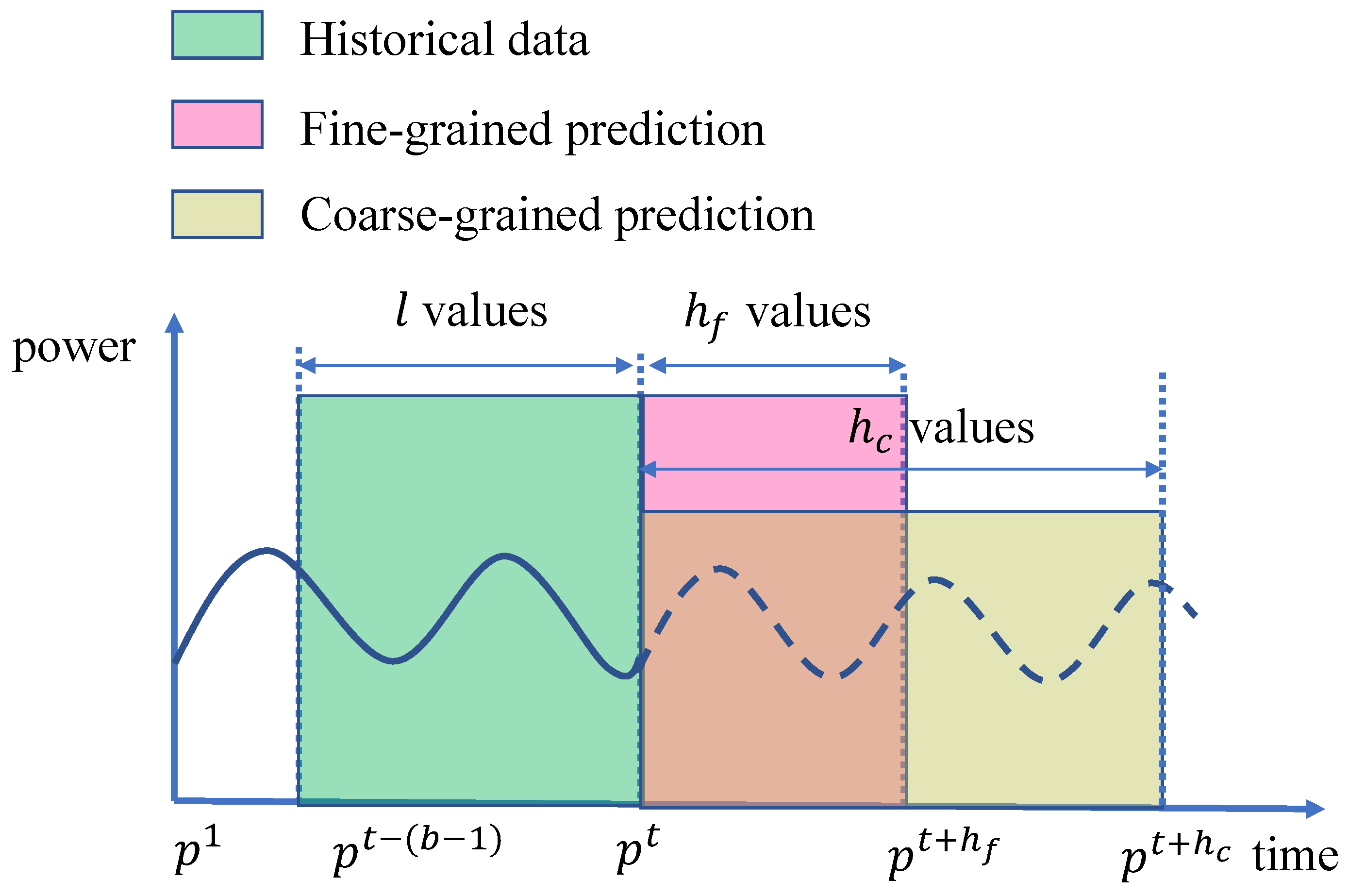
There are two power consumption prediction problems in daily data center operations [4], i.e., fine-grained prediction and coarse-grained prediction, as shown in Figure 1.

Fine-grained power consumption prediction is to predict the power consumption of a certain number of timestamps in the future, where the number of timestamps to be predicted is relatively small. It is also called multi-step prediction, which can be formulated as below, where f is the fine-grained prediction model and $h_f$ is the number of timestamps, i.e., the prediction horizon.

$$[p^{m+1},\dots ,p^{m+h_f}]=f(p^{m-(l-1)},\dots ,p^m;U^{m-(l-1)},\dots ,U^m)$$

(1)

Coarse-grained power consumption prediction is to predict the average power consumption during multiple timestamps in the future, which is formulated as below. $f^{\prime }$ is the coarse-grained prediction model, and $h_c$ is the length of the future time interval corresponding to the average power consumption.

$$\left[{\overline{p}}^{(m,h_c)}\right]=f^{\prime }(p^{m-(l-1)},\dots ,p^m;U^{m-(l-1)},\dots ,U^m)$$

(2)

Notice that the predicted time interval is much longer than the time unit of power consumption series.

3. The Unified Power Consumption Prediction Framework

In this section, we propose the unified prediction framework for power consumption in daily data center operations. The prediction framework incorporates the historical power consumption series, and the URI requests a unified model for both fine-grained and coarse-grained prediction. The framework is also compatible with other non-intrusive features.

3.1. The Character-Level URI Representation

Before explaining our proposed prediction framework, we begin with the URI encoding strategy, which can generate informative embeddings of URIs. A URI example is as follows: http://www.wc98.com/english/competition/matchstat8877.htm.

The above URI is an address to a web page, also called a Uniform Resource Locator (URL). URLs are more specific types of URIs, and the string format of a URL is the same as the string format of a URI. We use URL here as an example to explain the URI encoding strategy.

As we can see, a piece of URI is in a fixed template, which consists of several parts, including the transfer protocol (HTTP (the Hypertext Transfer Protocol (HTTP) is an application protocol for distributed and collaborative systems, which defines how messages are formatted and transmitted)), the host name (www.wc98.com), the file path (English, competition), and the file name (matchstat8877.html). Given a piece of URI, we can decompose it into different parts according to the above template based on a separator slash “/”. We do not consider the powerful impact of different transfer protocols and the host name, because only the request contents in URLs are relevant to power consumption. In this way, a URI is now a set of keywords containing an accessing path and file name. If the URI corresponds to a web service, then the file name is the corresponding application name.

Now, we need to design a suitable representation for the keyword sets from URIs. Popular approaches of word embeddings can generate vector representations of words based on their co-occurrences in a large corpus. These word embeddings could capture the semantic meaning of words, but they are not applicable in the URI domain. On the one hand, the number of keywords in the URI domain is relatively small, and it is not clear that the-occurrence relationship could contribute to the power consumption prediction. One the other hand, although developers tend to use meaning words in paths or application names, there is still a large number of keywords that lie outside of the vocabulary. Inspired by the representation of RGB images, we propose to transform URIs at each timestamp into vector representations based on character frequencies.

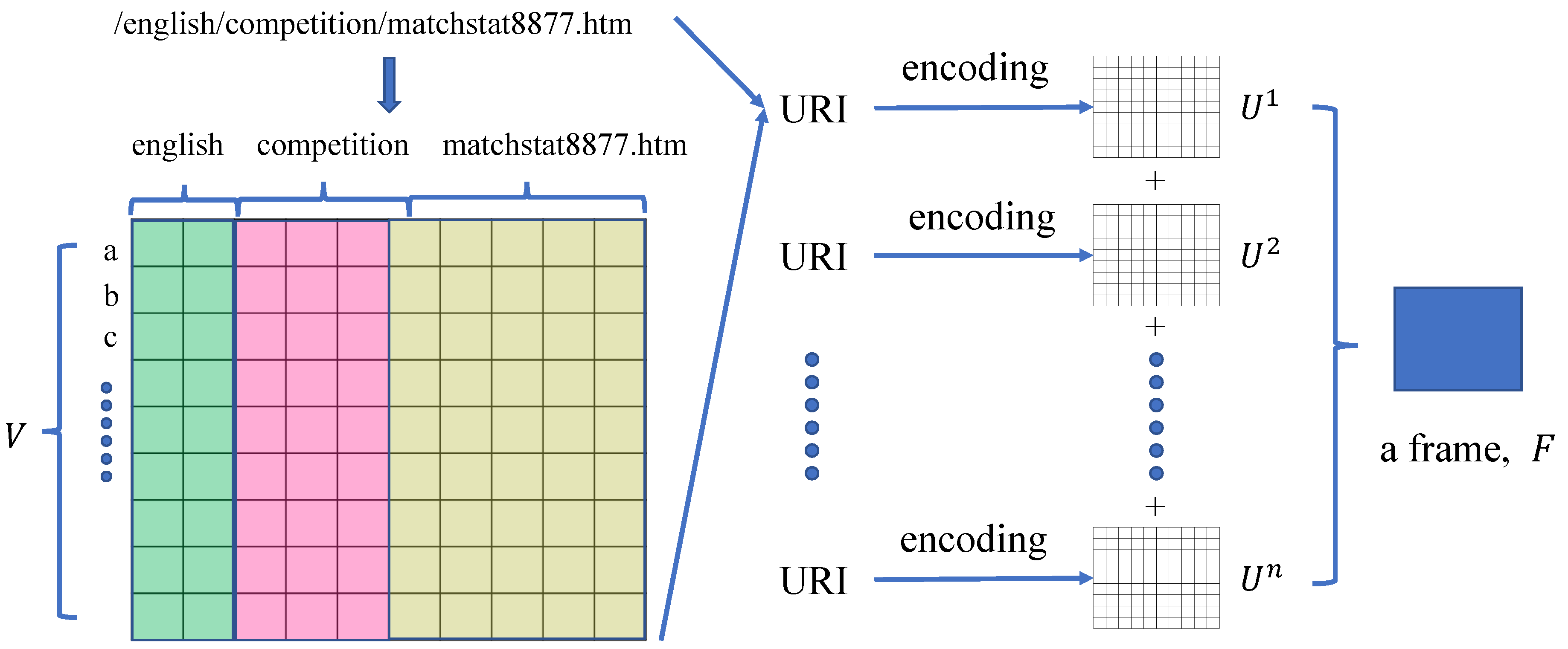
The encoding strategy of URIs is shown in Figure 2. We employ a character-level frequency encoding strategy in this paper. When decomposing URIs into keyword sets, for each keyword, we record its position in the URI. For example, in the above URI, the position of keyword “English” is 1, and the position of keyword “competition” is 2. Suppose the number of different positions is k, then we can obtain k keywords $[w_1,w_2,\dots ,w_k]$, from k different positions. We use $[l_1,l_2,\dots ,l_k]$ to denote corresponding word lengths. Moreover, we use V to denote the vocabulary of characters (alphabet) of size $\left|V\right|$. In this work, we use the vocabulary of 38 characters, including all lower case characters from the English alphabet, ten digit characters, underline, and period. The characters are shown below: $abcdefghijklmnopqrstuvwxyz0123456789\_.$

We use a character-level URI matrix $C\in {\mathbb{R}}^{\left|V\right|\times L}$ to represent a URI, where L is the summation of the length of the longest word in dictionary levels. Each column of C denotes a one-hot vector with respect to the alphabet V. Given character-level encoded URI matrices in a timestamp, we sum them up to obtain a character frequency distribution matrix, called a URI frame $F\in {\mathbb{R}}^{\left|V\right|\times L}$, where $F_{ij}$ denotes the frequency of occurrence of the i^th character in V at column j.

3.2. The Feature Extraction Network for URIs

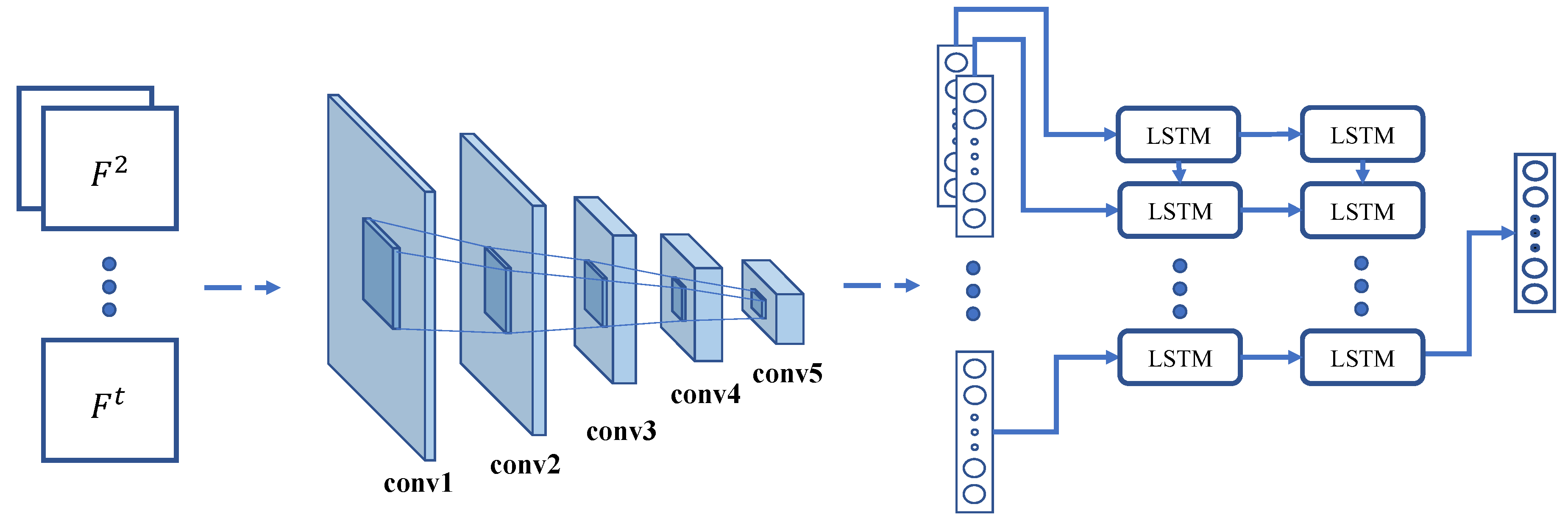
Combing Convolutional Neural Network (CNN) [9] and Long Short Term Memory (LSTM), we design a feature extraction network, which can extract both sequential and structural features from the matrices of encoded URIs.

We adopt CNN to extract structural features from the matrices of encoded URIs. CNN achieves the state-of-the-art performance in computer vision and speech recognition and is competitive in many NLP tasks [10,11]. By applying convolution operations (known as kernels or filters) at different levels of granularity, CNN can extract features that are useful for learning tasks and reduce the need for manual feature engineering. This characteristic is desired in our problem, where the goal is to extract useful structural patterns from URI frames between timestamp $t-(l-1)$ and timestamp t. These patterns serve as the input features in the prediction model.

The detailed configuration of the architecture for URI feature extraction is shown in

Table 1. The configurations of the CNN part.

Layer	Configuration
conv1	filter 8 × 38 × 11, stride 6 × 1, pad 1 × 1, LRN
conv2	filter 16 × 2 × 2, stride 2 × 2, pad 1 × 1
conv3	filter 32 × 2 × 2, stride 2 × 2, pad 1 × 1
conv4	filter 64 × 2 × 2, stride 2 × 2, pad 1 × 1, avgpool
conv5	filter 128 × 2 × 2
fc	128 × 64

. Filter specifies the number of convolution filters, whose receptive field size is denoted as “number × size × size”. Stride is the convolution stride, which is the interval when applying the filters on the input. Pad indicates the number of zeros to be added to each side of the input. LRN indicates whether to apply Local Response Normalization (LRN) [12], and avgpool indicates whether to apply average pooling layers. The last row in Table 1 is the dimensionality of the input vector and output vector in the fully-connected layer. We add a fully-connected layer to map the result of CNN to the desired feature vector with particular dimensionality. The activation function for all layers is Rectified Linear Units (ReLU) [12].

To keep the sequential nature of encoded URI frames, we extend the CNN for URI feature extraction by combining LSTM to exploit sequential features of URI frames, which have achieved impressive performance in different sequence learning problems [13,14,15,16]. LSTM is a type of Recurrent Neural Network (RNN) that captures sequential relevance. Note that LSTM incorporates memory cells that allow the network to learn when to forget previous hidden states and when to update hidden states, given new information available. LSTM can exploit the sequential nature from URI frame series and overcome the difficulty in learning long-term dynamics. The detailed architecture of the URI feature extraction network is illustrated in Figure 3.

3.3. The Power Consumption Prediction Framework

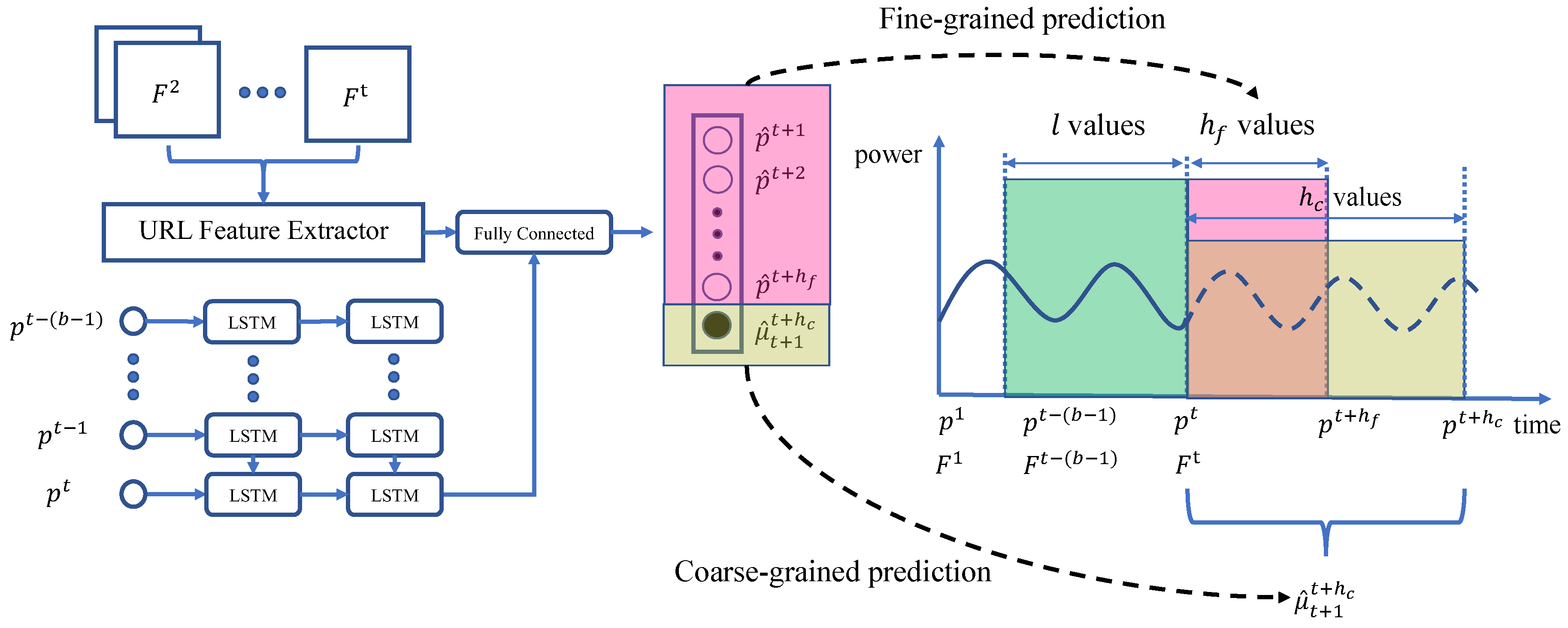
In this section, we propose a novel unified prediction framework, which predicts power consumption at both the fine-grained level and coarse-grained level simultaneously. The detailed architecture of the proposed prediction framework is presented in Figure 4.

There are two branches, the URI branch and the power consumption branch, which are related to the URI frame series and the power consumption series, respectively. In the URI branch, the CNN part of the URI feature extraction network follows the same architecture configurations as illustrated in Table 1, and we use a two-layer (chosen empirically) stacked LSTM network to extract sequential characteristics of the URI frame series with 256 memory units in each layer. Similarly, in the power branch, we use a two-layer (chosen empirically) stacked LSTM network to extract sequential characteristics of the power consumption series with 256 memory units in each layer. Finally, the outputs from these two branches are tied together by adding a fully connected layer on top of them.

In the output layer, the first few (equal to the width of fine-grained prediction window length) items are used for fine-grained power prediction, and the last item is used for coarse-grained power prediction. More specifically, if the width of fine-grained and coarse-grained forecasting window are $h_f$ and $h_c$, respectively, then the output layer will have $h_f+1$ items, where the first $h_f$ items in the output, $[{\widehat{p}}^{t+1},\dots ,{\widehat{p}}^{t+h_f}]$, denote the predicted power consumption values in the time period from timestamp $t+1$ to $t+h_f$. The last item of the output, ${\widehat{\mu }}_{t+1}^{t+h_c}$, denotes the average power consumption value from timestamp $t+1$ to $t+h_c$.

Traditional power consumption prediction methods iteratively perform one-step-ahead prediction up to the desired prediction horizon, resulting in prediction error accumulation. Unlike them, the proposed framework can predict fine-grained power consumption values and a coarse-grained average power consumption value simultaneously, which is more efficient and effective than traditional methods in terms of time complexity and prediction accuracy.

3.4. The Learning Algorithm

Our prediction model handles fine-grained and coarse-grained power prediction problems simultaneously, and naturally, we use the following two loss functions to compute the overall loss for each time series. We adopt Mean Square Error (MSE) as the loss function for the fine-grained power consumption prediction, which is defined as follows:

$${\mathcal{L}}_f=\frac{1}{N}\sum _{i=1}^N\sum _{j=t+1}^{t+h_c}\left|\right|\widehat{p^j}-p^j{\left|\right|}^2$$

(3)

where ${\widehat{p}}^j$ and $p^j$ denote the predicted value and the real value of power consumption, respectively. N is the number of training samples. For coarse-grained power consumption prediction, the corresponding MSE-based loss function is:

$${\mathcal{L}}_c=\frac{1}{N}\sum _{i=1}^N\left|\right|{\widehat{\mu }}_{t+1}^{t+h_c}-{\mu }_{t+1}^{t+h_c}{\left|\right|}^2$$

(4)

where ${\widehat{\mu }}_{t+1}^{t+h_c}=\frac{1}{h_c}{\sum }_{i=t+1}^{t+h_c}{\widehat{p}}^i$ is the predicted average power consumption value and ${\mu }_{t+1}^{t+h_c}=\frac{1}{h_c}{\sum }_{i=t+1}^{t+h_c}{p}^i$ is the real average value of power consumption.

Then, the overall loss function can be written as:

$$\mathcal{L}={\mathcal{L}}_f+\alpha \ast {\mathcal{L}}_c$$

(5)

where $\alpha$ is a hyper-parameter to balance the two loss functions.

The parameters of the entire network are jointly optimized. The detailed training process is shown in Algorithm 1. The inputs are power consumption series $L_p=[p^1,\dots ,p^m]$ and the corresponding URI set series $L_u=[U^1,\dots ,U^m]$. URI set series are encoded into URI frame series $L_f=[F^1,\dots ,F^m]$, based on the encoding strategy introduced in Section 3.1, Then, we employ a sliding window of length $n+h_c$ to generate N training samples. For each training sample $(X_t,y)$, $X_t$ contains two parts: the historical power consumption series $[p^{t-(b-1)},\dots ,p^t]$ and the URI frame series $[F^{t-(b-1)},\dots ,F^t]$. $y_t$ is the power consumption vector $[p^{t+1},\dots ,p^{t+h_f},{\mu }_{t+1}^{t+h_c}]$, where the first $h_f$ item is the real power consumption values and the last item is the average value of real power consumption.

Algorithm 1: The learning algorithm.

4. Experimental Evaluations

In this section, we evaluate the proposed prediction model, denoted as URL-LSTM, with other baseline algorithms, including Random Forest Regression (RF) [17], Support Vector Regression SVR [18], Long Short Term Memory (LSTM) [19] and Residual Recurrent Networks (RRN) [20]. We do not compare our proposed method with other power consumption prediction approaches in which intrusive features are needed. The analysis of the contribution of both non-intrusive and intrusive features in power consumption prediction is a potential future direction.

4.1. Data Simulation and Collection

Because URI requests are highly related to business processes of various companies, they are particularly sensitive in modern data centers, as well as power consumption statistics. Due to the extreme difficulty in acquiring these data, in this paper, we conducted our experiments based on synthetic datasets. Specifically, we employed a URL request dataset to simulate the URI requests to collect the synthetic data.

The World Cup 98 (WC98) dataset [21] collected all URL requests made to the World Cup website between 30 April 1998 and 26 July 1998. In the WC98 dataset, there were 33 different web servers at four geographic locations: Paris, France; Plano, Texas; Herndon, Virginia; and Santa Clara, California. To generate the synthetic data, we hosted the real web site of World Cup 98 on a server and simulate the requests from a client machine, based on these real requests. A Power Distribution Unit (PDU) was connected to monitor the power consumption of the server per second during the request simulation.

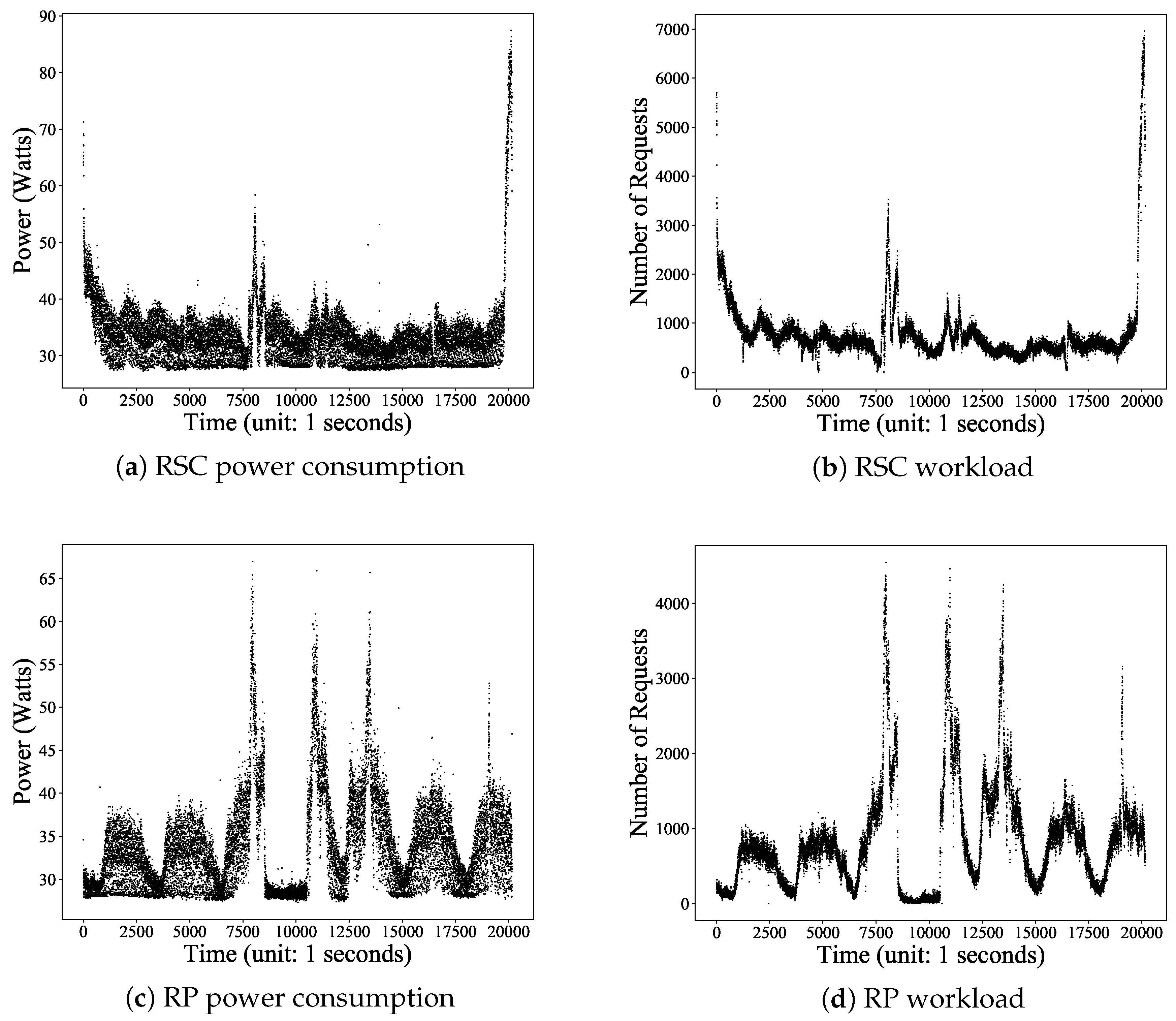
The original web servers hosting the World Cup 98 website were slow, compared with modern web servers. Therefore, we combined the requests to servers in the same location to simulate the URI visit. We selected two subset from the WC98 dataset. The first dataset contained all requests to the servers in Santa Clara from 1 July to 7 July, denoted as RSC. The second dataset contained all requests of the servers in Paris from 8 June to 14 June, denoted as RP.

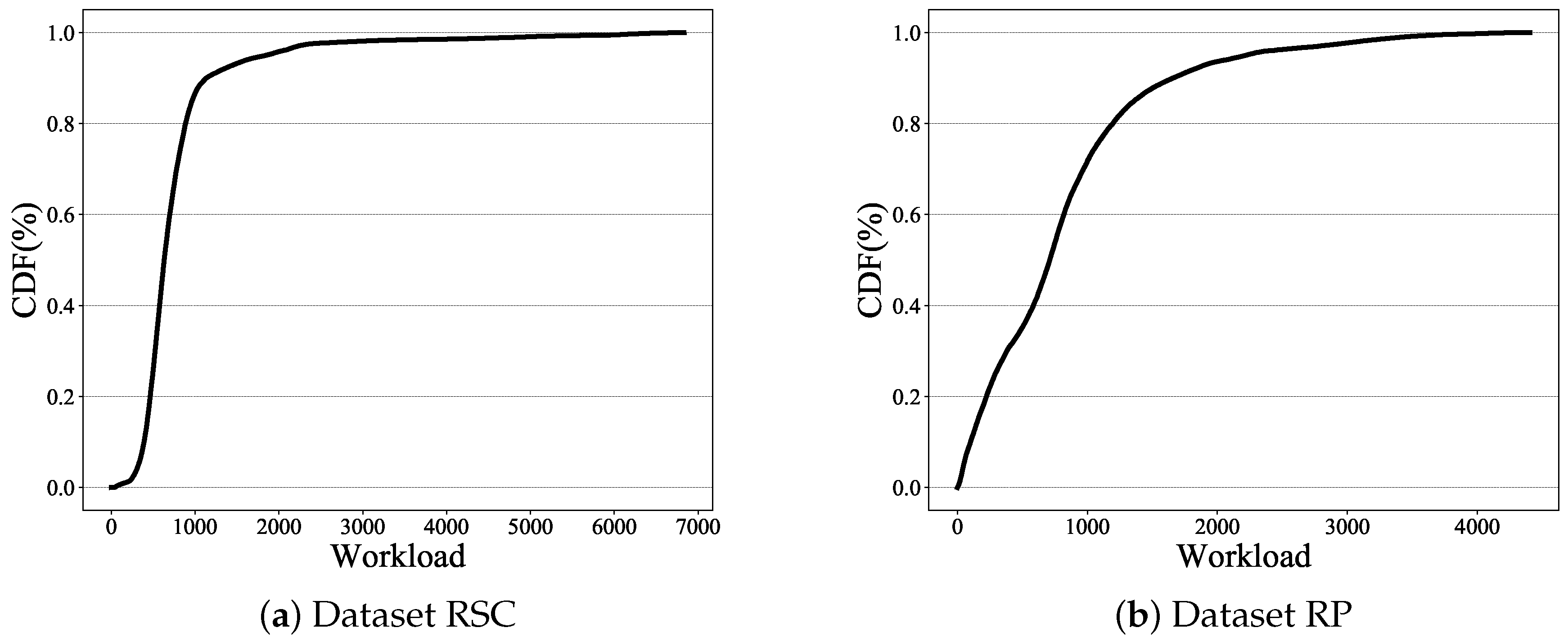
The power consumption series and the corresponding request workload series of dataset RSC are shown in Figure 5a,b, respectively. Those of dataset RP are shown in Figure 5c,d. As we can see, the power consumption series of RP fluctuated more drastically and had more peaks than those of RSC. These figures demonstrate that the power consumption in the data center had various circumstances with different characteristics. To show the characteristics of workload distribution in detail, we present the Cumulative DistributionFunction (CDF) of the request workload in Figure 6. We sorted in descendent order the timestamps based on the number of requests that happened at each timestamp. Figure 6 shows that timestamps with a large number of requests only took up around 20% of all timestamps.

4.2. Data Preprocessing

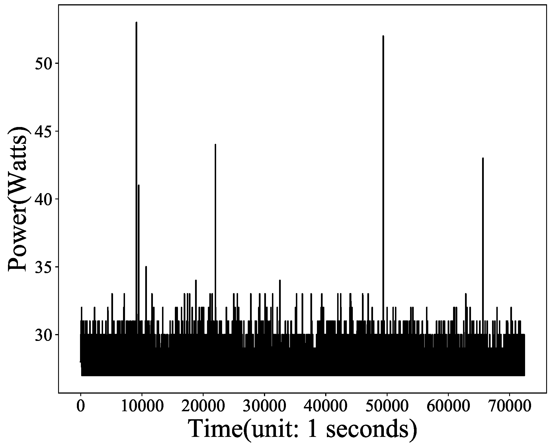
There were white noises in the power consumption series. Figure 7 presents the power consumption series of the server used in the experiments when the workload on it was empty, i.e., there was no URI request. As shown in Figure 7, the power consumption of the server was not stable, so we employed the moving average and downsampling to reduce the white noise. Given power series $[p^1,\dots ,p^m]$ and the length of the moving windows w, we calculate the moving average value for each power consumption value $p_t$ in the series as follows:

$$p_t=\frac{1}{w}\sum _{i=t-(\frac{w}{2}-1)}^{t+\frac{w}{2}}{p}^i$$

(6)

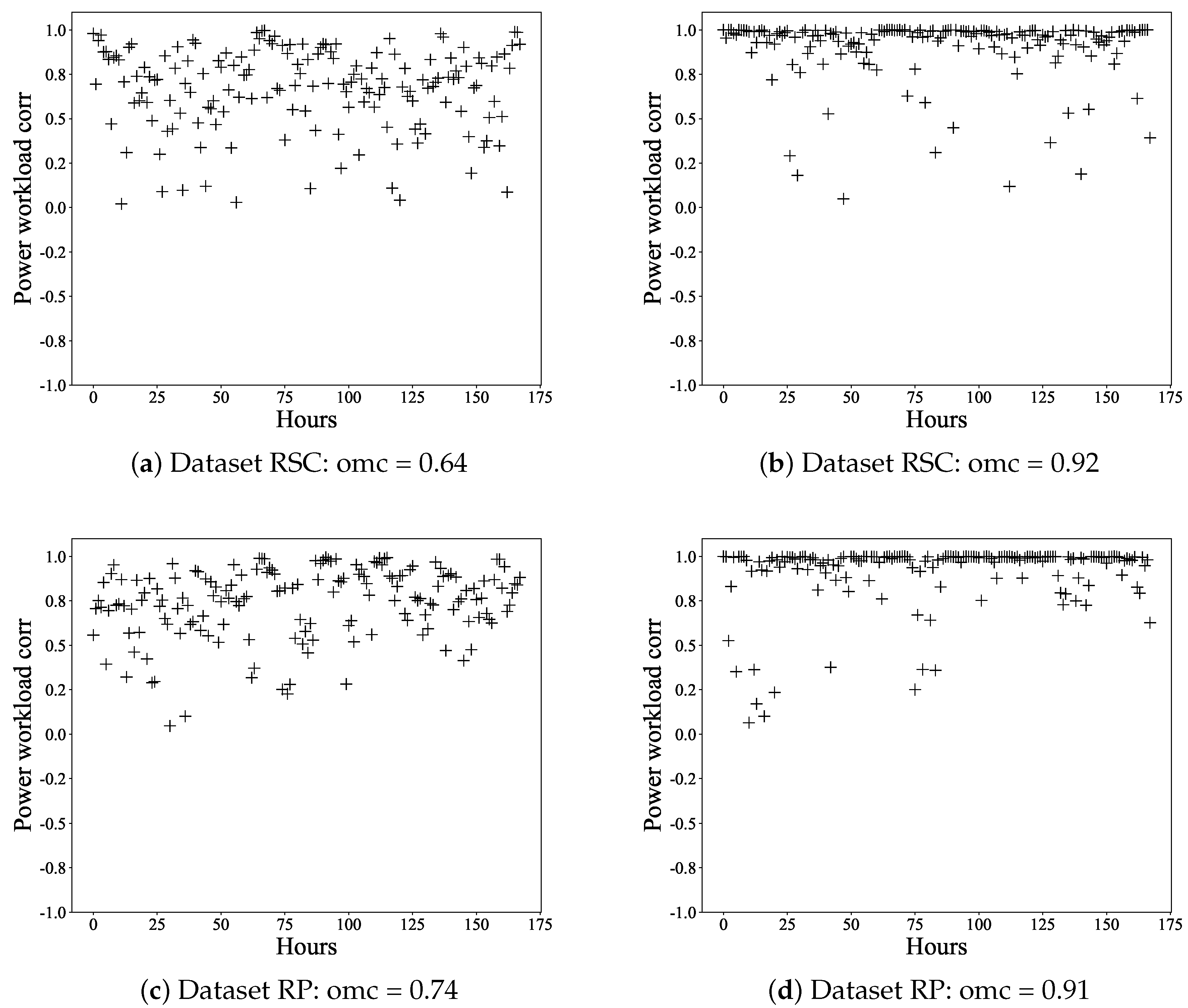
Through extensive experiments, we found that a moving window of size 20 could yield the best noise reduction performance. Then, we downsampled the smoothed power series with a non-overlapping adjacent window whose length was 30 s. We used Spearman’s rank correlation coefficient [22] to measure the correlation of the power consumption series and request workload series. The hourly correlations are shown in Figure 8, where Figure 8a,c is the correlations of the raw series and Figure 8b,d is the correlations of smoothed series. The overall mean correlation (omc) is noted in the caption of each figure. As we can see, after noise reduction, the correlation coefficients were improved significantly and close to one.

4.3. Experimental Settings

The experiment settings were as follows. We used a sliding window whose length was two days to segment dataset RSC and RP. The stride was one day long. Then, we could obtain 12 subseries, where six of them were from dataset RSC, denoted as RSC1 to RSC6, and the other six were from dataset RP, denoted as RP1 to RP6. The length of each subseries was two days, i.e., 48 h.

For each subseries, we used the first 36 h as the training data and the remaining 12 h as the testing data. The maximum number of training epochs was 100. For deep learning-based prediction models, such as LSTM, RRN, and the proposed method URL-LSTM, the learning rate was $\eta ={10}^{-4}$ from Epochs 1 to 50, and the learning rate was $\eta ={10}^{-5}$ from Epochs 50 to 100. The input window size b was 48; the prediction window size $h_f$ for fine-grained power consumption prediction was 10; and the prediction window size $h_c$ for coarse-grained power consumption prediction was 30. The hyper-parameter $\alpha$ was 0.5.

4.4. Fine-Grained Power Consumption Prediction

In this section, we report the experimental results of fine-grained power consumption prediction. We first present the Mean Relative Error (MRE) of the above five methods over six subseries of RSC and six subseries of RP. MRE is widely used as an evaluation measure to indicate the prediction accuracy among different prediction models. Given power consumption series $[p^1,\dots ,p^n]$ and predicted power consumption series $[{\widehat{p}}^1,\dots ,{\widehat{p}}^m]$, the mean relative error is defined as follows::

$$MRE=\frac{1}{m}\sum _{i=1}^n\frac{|p^i-{\widehat{p}}^i|}{p^i}$$

(7)

where m is the length of the series.

We computed the MRE of the 12 series for the five prediction methods. The results are shown in

Table 2. The MRE (%).

	RF	SVR	LSTM	RRN	URL-LSTM
RSC1	0.84	1.00	0.85	0.86	0.49
RSC2	5.66	2.59	1.47	0.93	0.52
RSC3	0.46	0.66	0.56	0.96	0.39
RSC4	0.68	0.57	0.26	0.29	0.20
RSC5	0.57	0.56	0.57	0.48	0.37
RSC6	13.51	8.04	2.89	3.13	0.37
RP1	0.52	0.53	0.36	0.34	0.26
RP2	12.15	4.50	3.17	0.89	0.63
RP3	0.37	1.16	0.43	0.75	0.33
RP4	0.45	0.99	0.53	0.40	0.35
RP5	0.42	0.66	0.50	1.04	0.36
RP6	1.02	1.06	0.88	0.68	0.31

, and the average MREs are shown in

Table 3. The average MRE (%).

	RF	SVR	LSTM	RRN	URL-LSTM
RSC	3.70	2.23	1.10	1.11	0.39
RP	2.49	1.48	0.98	0.68	0.37

. Best values are in bold. As is illustrated in Table 2 and Table 3, the proposed method outperformed the other four popular prediction methods significantly. Some series contained unexpected dramatic changes, such as RSC6 and RP2, which are presented in Figure 10c,e. In these series, the proposed URL-LSTM improved the MRE by around 3% compared to the deep leaning-based methods LSTM and RRN. Compared with the traditional methods RF and SVR, URL-LSTM improved 10%.

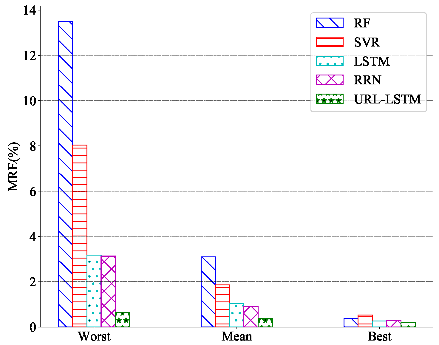
To provide an insightful analysis of the comparison, we show the best, the mean, and the worst prediction MREs of the five prediction methods among the 12 series in Figure 9. As we can see, LSTM, RNN, and the proposed URL-LSTM had better performance than the traditional methods such as RF and SVR. LSTM and RNN had similar MREs, while URL-LSTM outperformed all the other prediction methods in all three cases.

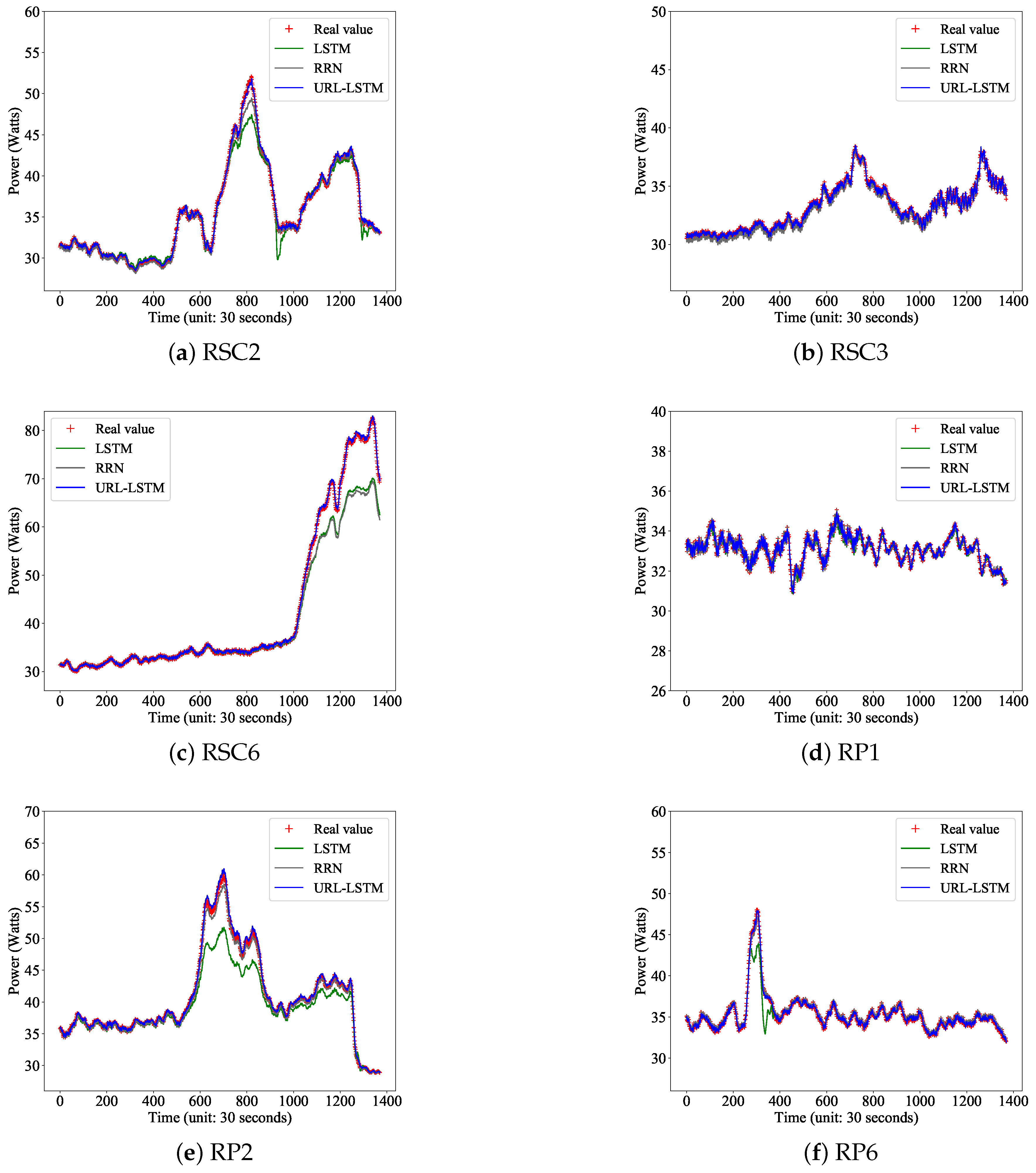
We report the predicted results of LSTM, RNN, and URL-LSTM, together with the original power consumption series in Figure 10. Please note that as illustrated in Table 3, LSTM, RNN, and the proposed URL-LSTM outperformed other traditional methods, so we only report the results of these three methods. To avoid redundancy, we only present the results of six series.

Figure 10 shows the prediction ability of these methods graphically. Figure 10a–c presents the prediction results of series RSC2, RSC3, and RSC6. We can see from these figures that when the power consumption fluctuates within a small range, all three methods, LSTM, RNN, and URL-LSTM, could predict the power consumption accurately. However, URL-LSTM had lower prediction MRE, according to Table 2. When the power consumption started to change dramatically, as shown in Figure 10c, the proposed URL-LSTM could efficiently track the dramatic change, while LSTM and RNN could not. We can observe similar results in Figure 10d–f, which presents the prediction results of series RP1, RP2, and RP6. Especially in Figure 10e, URL-LSTM performed other methods when there was a high power demand in the middle of the series.

Parameter Sensitivity

In this section, we study the performance of our proposed framework with respect to the length of the historical windows and the length of the prediction windows. Both are essential to the framework. Shorter historical windows mean fast training and prediction speed, while longer prediction windows make the proposed framework more applicable.

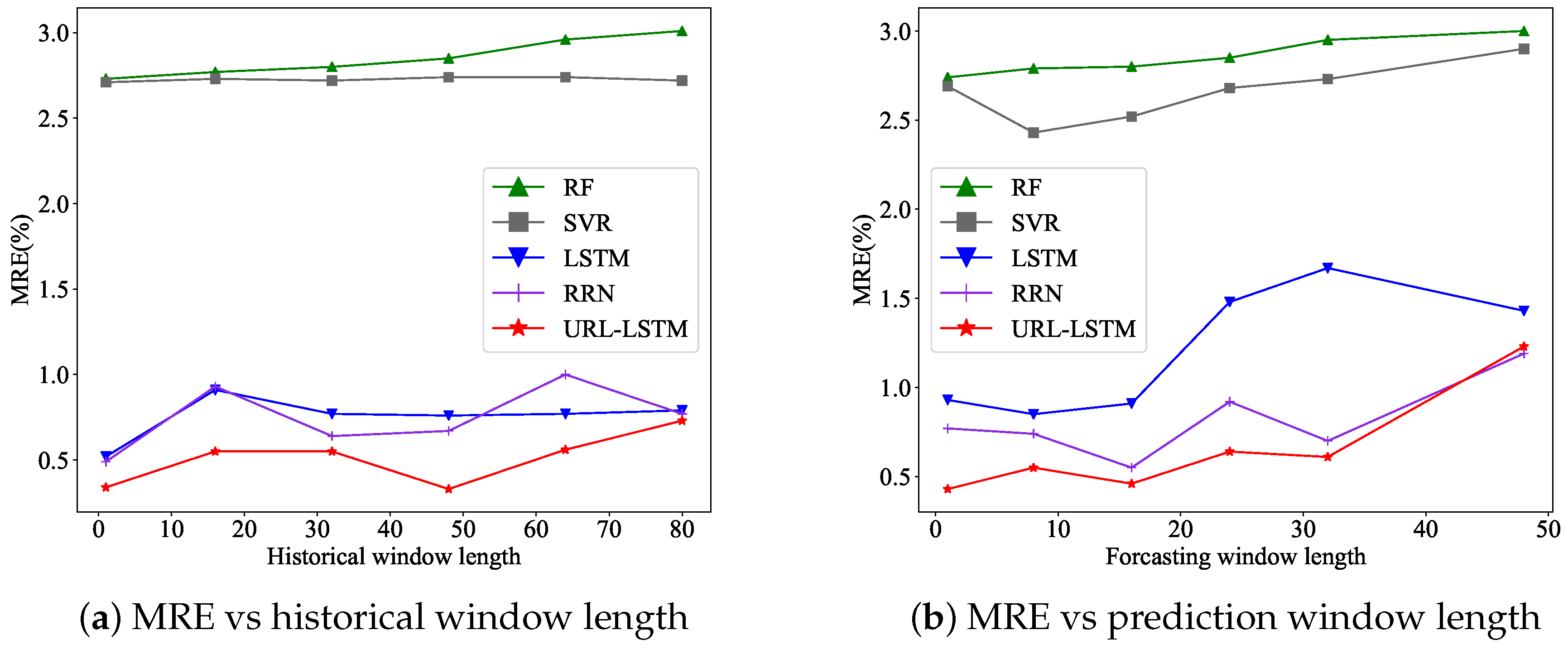
Figure 11a presents the average change of MRE on the 12 series for the five prediction methods, concerning the historical window length. Other settings remained the same as the ones in Section 4.3. We performed the experiments when varying the length of the historical windows as follows: 1, 16, 32, 48, 64, and 80. URL-LSTM achieved the best results when the length of historical windows was 48. As the length increased, LSTM, RNN, and URL-LSTM did not have a monotonous increasing or decreasing trend. Nevertheless, they remained at a low level of MRE. In general, the other four methods could not outperform URL-LSTM. On average, URL-LSTM reduced the MRE by around 0.5% compared to deep learning-based methods and around 2% compared to the traditional methods.

Figure 11b shows the average change of MRE on the 12 series for the five prediction methods, concerning the prediction window length. It is not surprising that all five methods had increasing MREs when prediction windows became longer, because of the accumulated error. The best prediction window length of the datasets used in the experiments was 16 time units, where each time unit was 30 s long, as mentioned.

4.5. Coarse-Grained Power Consumption Prediction

In the coarse-grained prediction, except the proposed URL-LSTM, the other four methods could not support fine-grained and coarse-grained power consumption prediction simultaneously. For these methods, we retrained their prediction models by using the training dataset where the predicted values were the average power consumption. The length of the historical window b was 60, and the length of the coarse-grained prediction window $h_c$ was ten time units.

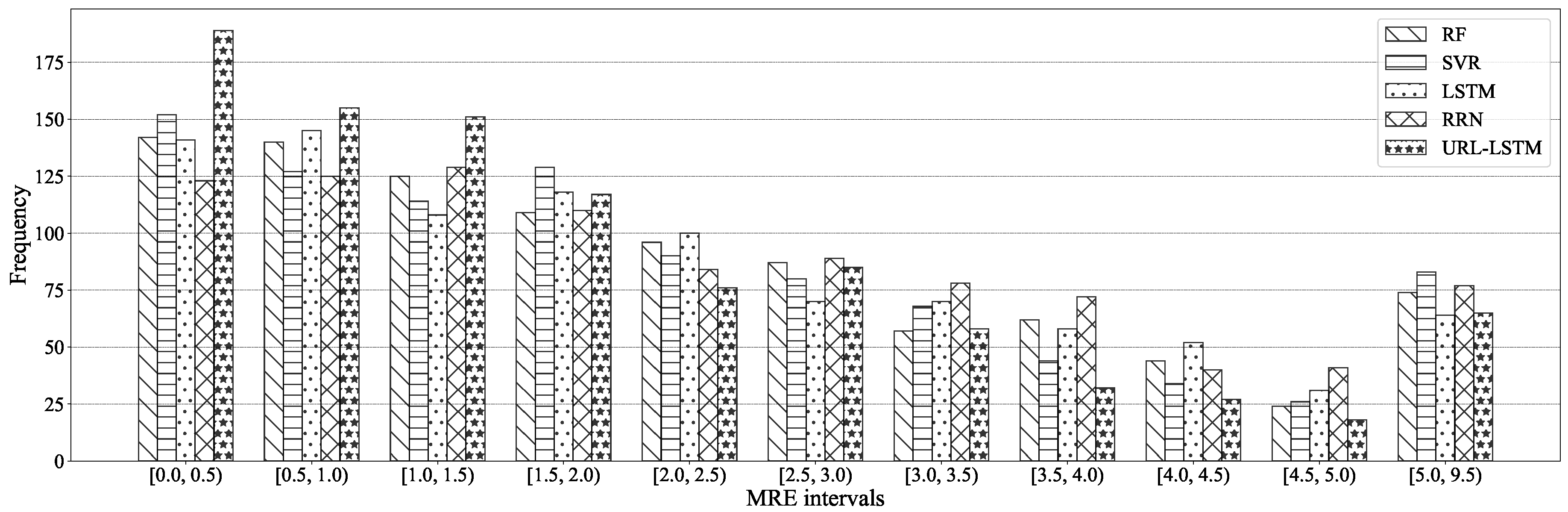
To give a detailed MRE distribution of the coarse-grained power consumption prediction, we present the histogram of MRE. The histogram shows the frequencies of MRE at different intervals when predicting the average power consumption of the next $h_c=10$ time units (300 s). As is illustrated in Figure 12, the proposed URL-LSTM efficiently reduced the MRE in the intervals whose MREs were large, such as [3.5%, 4.0%) and [4.5%, 5.0%). Furthermore, the frequency of URL-LSTM in the intervals that MREs were small, such as [0.0%, 0.5%) and [0.5%, 1.0%), were significantly larger than other methods.

The MRE distribution in detail is presented in

Table 4. The MRE (%) distribution in coarse-grained power consumption prediction.

Interval	RF	(Agg)	SVR	(Agg)	LSTM	(Agg)	RRN	(Agg)	URL-LSTM	(Agg)
[0,0.5)	14.79	(15)	16.05	(17)	14.73	(15)	12.7	(13)	19.42	(20)
[0.5,1)	14.58	(30)	13.41	(30)	15.15	(30)	12.9	(26)	15.93	(36)
[1,1.5)	13.02	(43)	12.03	(42)	11.28	(42)	13.3	(39)	15.52	(51)
[1.5,2)	11.35	(54)	13.62	(56)	12.33	(54)	11.36	(51)	12.02	(63)
[2,2.5)	10.00	(64)	9.50	(65)	10.45	(64)	8.68	(59)	7.81	(71)
[2.5,3)	9.06	(73)	8.45	(74)	7.31	(72)	9.19	(69)	8.73	(80)
[3,3.5)	5.94	(79)	7.18	(81)	7.31	(79)	8.05	(77)	5.96	(86)
[3.5,4)	6.46	(86)	4.65	(85)	6.06	(85)	7.43	(84)	3.29	(89)
[4,4.5)	4.58	(90)	3.59	(89)	5.43	(91)	4.13	(88)	2.77	(92)
[4.5,5)	2.50	(93)	2.75	(92)	3.24	(94)	4.23	(93)	1.85	(94)
[5,9.5)	7.71	(100)	8.76	(100)	6.69	(100)	7.95	(100)	6.68	(100)

. Here, we present the average MRE value of each prediction method at each interval. The column with brackets is the accumulated percentage for each MRE interval. As we can see, the proposed URL-LSTM accumulated much faster than other prediction methods, which revealed that URL-LSTM was a promising method with a stable prediction ability.

5. Related Work

The power consumption prediction is close to the multivariate time series prediction problem. In this section, we first summarize some related works of power consumption estimation, followed by deep learning-based methods of multivariate time series prediction. Methods based on deep learning in multivariate time series predictions resulted in better performance recently, and we do not include traditional time series prediction methods in this section to avoid redundancy, which readers can find in many related surveys.

5.1. Power Consumption Estimation

Usually, power consumption estimation is based on the configurations of the servers or the status of the servers. Configuration-based power estimation calculates the power consumption based on the static mathematics models of the configurations of the servers. According to previous studies [5,6,7], power consumption estimation is performed at the processor level, server level, and data center level. Processors take up a large part of the overall power consumption of servers, so estimating the power consumption of processors can be used as the overall power consumption roughly. Comprehensive power consumption models of processors rely on specific details of the process architecture to achieve high estimation accuracy [23,24,25]. The main components in the IT infrastructure of data centers are servers. Economou et al. [26] proposed a non-intrusive model for real-time server’s power estimation. Most power consumption in data centers is by the servers. There are three types of power consumption models at the data center level, i.e., power models based on queuing theory [27], power models based on power efficiency metrics [28], and other various power models [29,30].

Status-based power estimation can be categorized into two kinds, i.e., explicit models and learning-based models, all of which focus on how to build models for power consumption series from data centers. Explicit models exploit the characteristics of the power consumption series to build power estimation models with the help of traditional time series models. Learning-based methods utilize machine learning techniques to predict power estimations. For example, Tesauro et al. [8] presented a reinforcement learning approach to manage server performance and power consumption online simultaneously. Li et al. [4] proposed a systematic power prediction framework based on extensive power dynamic profiling and recurrent deep learning models.

The configuration-based power estimation can only provide a general picture of power consumption in data centers, which is useful during designing and planning data centers. In the daily data center operations, the configuration-based power estimation is not helpful. Status-based power estimation, on the other hand, benefits the daily data center operations, because it considers the working status of servers, clusters, and data centers. Almost all existing approaches in the category require agent deployment in servers to monitor and collect various features, such as CPU usage, storage usage, and network IO, which brings extra efforts of agent deployment or feature collection burden to the data centers. In some working environments, the agent deployment could also cause security issues. In our proposed power consumption prediction method, as mentioned, we only used non-intrusive features, i.e., the workload of URI requests. Unlike all these existing approaches, our proposed method could accurately predict power consumption without bringing extra burden.

5.2. Deep Learning-Based Prediction of Multivariate Time Series

The time series prediction problem has been prevalent for decades and attracted much research efforts from many application domains. Power consumption prediction is one of them. Traditional models for time series prediction, such as ARMA, are not suitable for nonlinear multivariate times series. Recently, more attention has been laid on prediction methods based on deep learning. Deep learning-based methods employ deep neural networks to simulate the nonlinear relationship structure to obtain better prediction accuracy for multivariate time series. Recurrent architectures are suitable for tasks with sequence modeling. However, the traditional RNNs are often disturbed by gradient vanishing and gradient explosion in the training process [31]. LSTM has proven to be a promising method for sequence modeling, which contains a selective memory function [32] and can resolve the gradient related issues of RNNs. However, beyond the good results of LSTM, training RNN with LSTM cells requires a carefully designed optimization procedure [33,34,35]. Residual Recurrent Networks (RRN) are inspired by the Residual Network (ResNet) [36], which incorporate the residual connecting mechanism into RNNs, resulting in fewer hidden units, a fast training speed, and better prediction performance than vanilla RNNs.

The above deep learning-based prediction approaches studied how to constructive various new neural network architectures or processes for multivariate time series prediction. Unlike them, we, in this paper, focused on how to utilize non-intrusive features to help power consumption prediction. It is worth mentioning that our proposed framework is compatible with many other deep neural networks besides LSTM.

6. Conclusions

In this paper, we studied the problem of predicting power consumption in data center operations. By carefully analyzing the desired properties of an applicable prediction framework, we proposed a non-intrusive, traffic-aware prediction framework for power consumption. The proposed framework could predict the power consumption at both fine-grained and coarse-grained levels by using only non-intrusive features. To the best of our knowledge, we are the first to use only non-intrusive features for power consumption prediction in data center operations. We also designed a novel character-level encoding strategy for URIs to obtain a descriptive representation. The proposed framework incorporated the URI frames and the power consumption series by using convolutional and recurrent neural networks. We compared with several other popular prediction approaches, and the experimental results showed that the proposed framework outperformed them significantly.

The paper provided a solid starting point for non-intrusive power consumption prediction. There are several other non-intrusive features available in data center operations, such as docker configurations and workflow specifications. The future direction is to consider multiple heterogeneous non-intrusive features to improve the prediction performance further.