Abstract
Metamodels proved to be a very efficient strategy for optimizing expensive black-box models, e.g., Finite Element simulation for electromagnetic devices. It enables the reduction of the computational burden for optimization purposes. However, the conventional approach of using metamodels presents limitations such as the cost of metamodel fitting and infill criteria problem-solving. This paper proposes a new algorithm that combines metamodels with a branch and bound (B&B) strategy. However, the efficiency of the B&B algorithm relies on the estimation of the bounds; therefore, we investigated the prediction error given by metamodels to predict the bounds. This combination leads to high fidelity global solutions. We propose a comparison protocol to assess the approach’s performances with respect to those of other algorithms of different categories. Then, two electromagnetic optimization benchmarks are treated. This paper gives practical insights into algorithms that can be used when optimizing electromagnetic devices.
1. Introduction
The increasing constraints on the design of electromagnetic devices require numerical tools that can model the electromagnetic fields with high precision on local quantities. The Finite Element (FE) method is the most used method to satisfy such a requirement. However, this method may be costly in terms of computational time due to nonlinear behavior, 3D geometry, and time dependency. Thus, its usage for optimization, i.e., iterative process, should be made with caution since only a limited number of evaluations of the simulation tool is possible. It also suffers from numerical noise due to the remeshing when dealing with geometric parameters. Thus, these issues have been extensively studied in the literature using the metamodel approach and the stochastic algorithms [1,2], e.g., genetic algorithms (GA), etc. On the other hand, optimization using gradient-based algorithms is less studied due to the remeshing error that perturbs the gradient’s computation using the finite difference technique [3].
Metamodels are widely used in the context of optimization of electromagnetic devices [4,5]. They are constructed based on a small sample from the expensive model, i.e., FEM simulation. The optimization is performed on the metamodel rather than the expensive model. This metamodel could be improved using infill criteria that enable the sampling of new promising designs from the full model. The infill criterion has a strong influence on how efficiently and accurately the algorithm locates the optimum.
In this paper, we developed a new approach to the usage of metamodels in optimization because the conventional approach of fitting one metamodel and enriching it has some drawbacks:
- The infill criteria that focus more on the local search tend to sample points close to each other, which decays the conditioning of the correlation matrix and, consequently, the construction of the metamodel [6,7].
- The number of samples exponentially increases as the optimization problem’s dimensionality does (the curse of dimension). Thus, the size of the correlation matrix increases and consequently the time needed to fit the metamodel. This time can even exceed the evaluation time of the FE model.
- The infill criteria optimization problem is highly multimodal, and their modality is highly correlated to the sample size of the expensive model evaluations; when the number of samples increases, the number of local optima increases too. Therefore, it becomes highly difficult to solve these optimization problems [8].
- When dealing with constrained optimization, the infill criteria tend to sample inside the feasible region but not on the feasibility boundaries, which affects the solution accuracy [9].
This paper proposes a novel approach that considers the FEM simulation as a black-box and constructs cheap metamodels to reduce the computational burden while refining in regions with a high error or low objective value. Then we compare it to different approaches that directly use the expensive model; a derivative-based algorithm that uses the derivatives computed using the adjoint variable method and derivative-free ones such as GA and DIRECT [10,11]. The comparison mainly focuses on the implementation and the computational cost to get efficient results. Furthermore, we define metrics and a comparison protocol to ease this task.
The comparison results highlight the algorithms suitable for the optimization of electromagnetic devices and the pros and cons of each of them.
2. Metamodel Approach
The proposed approach is called Branch and Bound based on Metamodel (B2M2). It is based on the principle of the branch and bound algorithms and consists of a systematic enumeration of candidate regions by splitting the search space into smaller spaces. The algorithm explores each smaller space then estimates the upper and lower bounds for each one of them. A subspace is discarded if it cannot produce a better solution than the best found so far by the algorithm.
2.1. B2M2 Algorithm
We propose an algorithm that builds many metamodels, each on a specified region of the design space; each one of them is relatively easy to fit and is used to estimate the upper and lower bounds. Then, iteratively, it excludes the regions that are not promising. By adopting this algorithm, the drawbacks mentioned earlier are tackled, namely, the numerical ones related to the correlation matrix. The flowchart of the algorithm is shown in Figure 1.
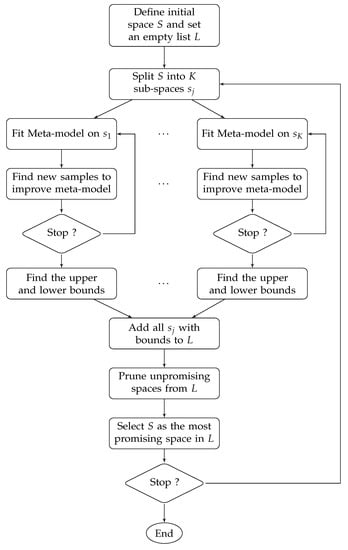
Figure 1.
Flowchart of B2M2.
2.1.1. Initialization
In the beginning, the initial space S is defined, and an empty list L is set. L will store the potentially optimal regions. Additionally, a maximum depth level l is defined to limit the exploration of the algorithm. The depth level can be seen as a metric of how many times the initial design space S can be subdivided.
2.1.2. Branching
The branching stands for subdividing the initial design space S. The most intuitive rule is splitting each dimension of S by two. This will lead to subspaces ( is the number of variables). Unfortunately, the number of subspaces increases exponentially as the number of variables grows. This is not desired, and a more practical rule is proposed.
For metamodels, the purpose behind branching is to improve upon its accuracy by reducing the size of the design space. Thus, the space S is split, such as the produced subspaces are of better accuracy. Therefore, the metamodel fit to S is used to identify the dimensions of high inaccuracy.
The stochastic term in the Kriging predictor enables the modeling of the error not captured by the regression term. The correlation function characterizes this term. Commonly, the exponential function is used to express the correlation between two points and , and it is given by
where is the evaluation of the expensive model at , is the number of variables, and are the parameters of the correlation.
The value of characterizes the smoothness of the function, while the values of enable the modeling of the changes over distance. Large values of serve to model rapid changes even over small distances. Hence, the values of are indicators of how the function varies.
If the value of , corresponding to a variable , is the largest. Then, the change in the ith-dimension is more important than other dimensions (when the variables are normalized). Consequently, splitting the space S by dividing its dimension i will lead to metamodels on the subspaces that are better than the one on S.
A simple example is used to test this property of the Kriging model (2). The studied function is a three-dimensional one but depends explicitly on only two variables, and one of them presents more variation than the other. In this example, we expect the value of to be higher than and . So, a Kriging model is fitted to a Design of Experiment (DoE) of 15 samples (five times the number of variables).
Indeed, the metamodel fitting led to , which confirms the proposed idea. Ordering the value of will lead to the variables that have the highest variation. The function does not depend on then which is the smallest allowed value for .
More than one variable can be chosen for separation; these variables are picked in the decreasing order of their corresponding values. Each variable is then subdivided into two parts which will lead to subspaces, where is the number of variables picked.
2.1.3. MetaModeling
Once the subspaces are determined using the branching rule (see the previous section), Kriging models are built for each one of them. The initial DoE, such as Hammersley, Latin Hypercube Sampling (LHS), etc., is determined, and the black-box-model is evaluated.
Additional samples are added using infill sampling criteria (ISC) to improve the metamodel approximation. The choice here is crucial for estimating of the bounds and rely on the prediction error. New samples are added—where the prediction error is high—that consequently improve the metamodel globally on the subspace. Additionally, a limited number of points are sampled using the expected improvement (EI) criterion to enhance local exploitation (or EI subjected to the constraints metamodel for constrained problems). This will also improve the global performance of the algorithm.
2.1.4. Bounding
Once the metamodel is fit to each subspace, we look for the lower and upper bounds on each of them as the Kriging can give the predictor and its error estimation. The Kriging model is constructed based on the assumption that the prediction is normally distributed with mean and standard deviation [1].
The aim is to find the interval that enclose the solution on a subspace given a specified probability, e.g., corresponds to a probability of 99.73% that the solution is enclosed between the bounds. We exploit this feature for the computation of bounds using the following formulations (3) and (4):
where and are the predictors of the objective function f and the constraints respectively and , are their error estimations given by the Kriging metamodel. The parameter k can be seen as the confidence level required.
A smaller value of k reduces the probability of bounding the solution. It, therefore, increases the risk of eliminating a promising subspace. In contrast, higher values of k widen the bounding interval , which makes the elimination more difficult.
The optimization problems (3) and (4) have to be solved using appropriate optimization algorithms due to the multimodal behavior introduced by the terms. We use sequential quadratic programming (SQP) from Matlab for this task improved by a parallel multistart strategy with points uniformly spread on the design space. The number of starting points is much higher than the number of samples of the black-box model. Additionally, the gradient information is computed easily from the metamodel, then it is exploited to increase the efficiency of the SQP algorithm.
The optimization problem (4) can present difficulties in solving since the objective function and constraints are mostly concave. Furthermore, our experience has shown that is, most of the time, equal to the best-sampled point (the point that has the smallest value of the objective function and satisfies the constraints). Thus, this optimization can be discarded, and is set to be equal to the sample having the smallest value of the objective function and satisfying the constraints on the subspace. When no feasible sample is available for highly constrained problems, is set to be equal to a large value.
In most constrained optimization problems, the problem (3) may not have a solution on some subspaces. It means that these subspaces have no potentially feasible solution, and therefore the values of the bounds are set to some high value.
2.1.5. Elimination
The subspaces are added to L with their lower and upper bounds. A comparison between the newly added subspaces to L and the existing ones is conducted to eliminate those that cannot produce a better solution.
First, we set as the smallest upper bound of all the spaces in L, and then, we prune the spaces from L that have a lower bound that is greater than .
2.1.6. Selection Priority
The remaining subspaces in L are all promising ones; thus, one of them has to be chosen for the next iteration to be subdivided. Many strategies could be considered: by preferring depth-first for prioritizing local search or breadth-first for prioritizing exploration of the search space. In our work, we use the best-first; it is based on the lower bound of the objective function on the subspaces. Indeed, the subspace chosen from L has the smallest lower bound, and its depth level is smaller than the maximum specified depth level.
This strategy will prioritize subspaces that have the maximum potential for providing the best solution without any criteria on the size of the subspace.
The subspaces that have attained the maximum allowed depth level are stored in a list .
2.1.7. Termination
The algorithm will naturally iterate until the list L is empty. It is challenging to develop a robust termination criterion. However, the exploration of a subspace can be stopped if the difference between its lower bound and upper bound is less than a small threshold specified by the designer. It remains possible to stop the algorithm by setting a maximum number of evaluations of the black-box model.
The list contains the remaining subspaces that are at the maximum specified depth level, or their bounds are close. One should investigate them and search for the optimum in one of them without considering the prediction error. Otherwise, the algorithm could be restarted with the list and a higher maximum depth level if no solution is found.
2.2. Test Function
The Rosenbrock function is used as a test problem for this optimization algorithm. As shown in (5), the problem can be extended to many variables. Here we treat the bidimensional problem ().
Rosenbrock problem has one global minimum at and .
The setup of the algorithm parameters is as follows.
- The maximum depth level is .
- On each subspace, the initial sample is chosen using Hammersley sequence with 4 sample points, the same number of sample points is added using the prediction error as an ISC and two points are added using EI.
Figure 2 shows the evolution of the subspace division. As shown, we compute the lower and upper bounds for each subspace, i.e., and , respectively. The new subspaces are compared with those in the list L to discard the unpromising ones. The shaded area shows the subspaces discarded from the list L.
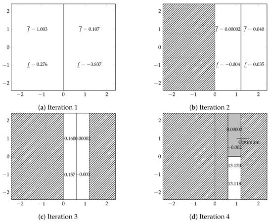
Figure 2.
Space exploration by the algorithm.
After only four iterations, the algorithm has located the subspace where the optimum lies. The grey region is the only space that was left in the list L.
To locate the solution in the remaining space, we consider only the predictor of the objective function and the constraints without their prediction errors. Then, we solve the optimization problem defined by these predictors to find the minimum. The solution found is close to the global minimum of the problem.
3. Expensive Model Approaches
In these approaches, we can distinguish two categories:
3.1. Derivative-Free
Derivative-free optimization is a discipline in mathematical optimization that does not use derivative information in the classical sense to find optimal solutions. Many gradient-free algorithms are designed as global optimizers and thus can find multiple local optima while searching for the global optimum. Various gradient-free methods have been developed. We investigate some of the most commonly used algorithms: genetic algorithm (from Matlab) and DIRECT algorithm [11].
A genetic algorithm is a stochastic optimization method based on randomness inherent in its operators: selection, mutation, and crossover.
The DIRECT method is one of the strategies for deterministic global optimization. It performs a systematic search of the design space using a hyperdimensional adaptive meshing scheme. Then it explores all the design space to find the optimum.
3.2. Derivative-Based
In design optimization, the gradient enables computing the search direction for gradient-based algorithms, e.g., sequential quadratic programming, active set. When dealing with FEM models, the gradient information is not always available.
3.2.1. Finite-Difference
The gradient can be approximated using finite-difference. However, numerical noise due to remeshing makes this approximation highly sensitive and requires adjusting the step size used for the computation [3]. Thus, the use of such an algorithm is not beneficial and a gradient of good quality need to be computed.
3.2.2. Adjoint Variable Method
The adjoint variable method (AVM) enables to efficiently compute the gradient from FEM code. Thus, no numerical noise due remeshing is observed as opposed to finite-difference. We implemented a 2D FEM code and an AVM code based on the discrete approach [12] for the gradient computation. The implementation of the AVM code is cumbersome since it requires intrusive manipulation of the FEM code itself. Nevertheless, it remains particularly appealing in terms of the computational cost, as the time for computing the gradient is equivalent to evaluating FEM code once whatever the number of variables. This can be very advantageous when treating large-scale problems, e.g., eight variables and more.
3.2.3. Globalization Strategy
Gradient-based algorithms suffer from the convergence to local optima that depends on the initial point. To handle this issue, a multistart strategy with uniformly distributed initial points is considered. By doing so, we increase the probability of attaining the global optimum.
Therefore, we define a convergence rate (C.R.) of the method. The C.R. is the proportion of optimizations that led to the best solution. Two solutions are considered the same if the distance between them is less than a small value. In this study, we took 1% of the design range.
4. Comparison Protocol
The comparison of the performance of different algorithms will be based on two criteria: the cost and the quality of the solution.
The quality of the solution stands for the value of the objective function found. The smaller, the better.
On the other hand, the optimization cost stands for the number of evaluations needed to attain the solution with a given probability. As we compare different approaches, we propose a probabilistic metric to measure the cost.
The convergence rate (CR) is the percentage of the number of runs that have converged to the best solution. The convergence rate concerns mainly SQP and GA since we perform multiple runs and the number of runs needed is unknown beforehand. To compute CR, we look among the solutions of each run for the best one (smallest value), then we count the number of runs that converged to that solution within a tolerance of 1% of the design range.
Once the convergence rate is determined, we assess the probability that at least one optimization leads to the best solution is
where n is the number of optimization runs to be considered.
If we want to consider a high probability () of finding the best solution, we can compute n the expected number of runs needed.
Then, the expected total number of evaluations (Expected # FEM evals) is n times the total average number of evaluations performed.
It should be noted that the cost of computing the gradient using the adjoint variable method is equivalent to evaluating the FEA once; thus, the # FEM evals are doubled for the SQP method.
5. Algorithms Settings
In this section, we present the configuration of the optimization algorithms. A set of parameters are defined based on our experience of using each algorithm.
5.1. B2M2 Algorithm
The branch and bound based metamodel (B2M2) algorithm is detailed in Section 2. Some options need to be configured, mainly the depth level and the number of FEA evaluations needed for fitting the metamodels.
Initial design: The initial design of each subspace is created using a space-filling LHS of size two times the number of variables. This may seem few, but as the algorithm progresses, the sample points of a parent space will be added to the initial design of its subspaces. Thus, the sample will grow as the subdivision of the space continues.
Infill points: Additional sample points are added in two different manners; the first one aims to explore the design space further and increase the metamodel precision by adding points where the prediction error is high. In contrast, the second one enables exploiting the best solution by adding new sample points that maximize the EI criterion.
The number of sample points added by each ISC is set to twice the number of variables. However, for EI, it may be stopped before this limit if there is no improvement in additional sampling points.
Globally, in each subspace, there will be sampled at most six times the number of variables.
Stopping criteria: The algorithm stops if a predefined depth level is reached. The maximum depth level is set to .
5.2. SQP Algorithm Assisted by Adjoint Variable Method
We use the SQP algorithm from the Matlab Optimization toolbox with the gradient of the quantities of interest computed using the adjoint variable method.
Multistart: To cope with the local search of the SQP method, we use a multistart strategy. We perform 100 runs with different initial points; these points are sampled using an LHS design to obtain a uniform distribution on the whole design space.
Stopping criteria: The stopping criterion is based on the StepTolerance option, meaning the algorithm stops when the relative change in the solution is less than .
5.3. DIRECT
We use DIRECT implementation of Finkel [11]. The default options are maintained except for the number of iterations.
Constraints: The constraints are handled by the penalty method by minimizing the penalized objective function
where is the penalty factor and has been chosen to be equal to 10.
Stopping criteria: The algorithm does not have an appropriate stopping criterion except the number of iterations and the number of evaluations. We stop the algorithm manually when there is no improvement in the objective function in 50 successive iterations.
5.4. Genetic Algorithm
We use the GA from the Matlab Global Optimization toolbox [10].
Multirun: As the inherent randomness in the genetic algorithm, meaning solving twice the same problem may not lead to the same solution, we adopted a multirun strategy by performing 50 runs of the algorithm.
Population: The population options are set as follows
- Size equal to 100 individuals for the unconstrained case and 200 for the constrained one.
- Selection function is uniform
- Crossover function is “scattered“
- Crossover fraction is 80% of the population
- Mutation function is Gaussian
- Elite fraction is 5% of the population
Constraints: The constraints are handled by the penalty method as defined in the article of Deb [13].
Stopping criteria: The algorithm is stopped if the value of the fitness function do not change during 50 generations.
6. Test Cases
6.1. TEAM Workshop Problem 25
In this test case, the device is used to orient the magnetic powder and produce anisotropic permanent magnets [14]. The magnetic powder is inserted into the cavity. The orientation and strength of the magnetic field should be controlled in order to obtain the required magnetization. A coil creates the magnetic field. The current density is fixed to A/mm2. The die press and electromagnet are made of steel with a nonlinear permeability. The geometry of the whole device is shown in Figure 3.
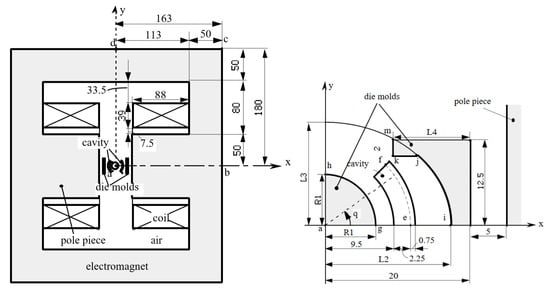
Figure 3.
Model of die press with electromagnet, (left) whole view (right) enlarged view [14]. Model of die press with electromagnet of TEAM problem 25
The shape optimization aims to obtain a flux density that is radial in the cavity space and with a constant magnitude of 0.35T. The objective function W is the sum of squared error between the and values sampled in 10 positions along the arc e–f shown in Figure 3.
where are the design variables (their bounds are shown in Table 1) and , . The flux densities and are computed by the FEA of the device.

Table 1.
Bounds of design variables for TEAM problem 25.
The results are summarized in Table 2.
Table 2.
TEAM Workshop problem 25 optimization results.
The genetic algorithm (GA) could not get reliable results; only one optimization converged to the solution shown in the table. Furthermore, this one is not competitive compared to other solutions. B2M2 can locate the optimal solution but with a higher cost, which is expected since it is based on branch and bound algorithms that enable to get reliable results. SQP and DIRECT algorithms gave the best solution, while the former outperforms all the others in terms of computational cost.
TEAM Workshop Problem 25 has a convergence rate (CR) of 34% when using the SQP method. This suggests that the optimization problem is not highly multimodal.
In terms of solution quality, SQP and DIRECT methods lead to the best solutions (smaller value of W), while SQP has a cost of almost seven times less than DIRECT.
B2M2 approach led to a competitive solution, even though the value of the objective function is a little higher. However, the design variables are very close to the ones found by SQP (difference of less than 1% of the design range). Most importantly, B2M2 cost is the most affordable.
6.2. TEAM Workshop Problem 22
The Superconducting Magnetic Energy Storage (SMES) device in Figure 4 consists of two concentric superconducting coils fed by currents that flow in opposite directions [15]. The inner coil is used for storing magnetic energy E, while the outer one has the role of diminishing the magnetic stray field computed on line a and line b.
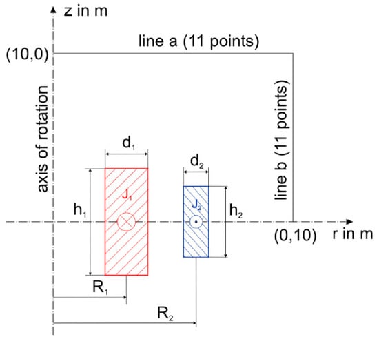
Figure 4.
SMES Device [15].SMES Device
The optimization problem’s goal is to find the design configurations (eight design variables) that give a specified value of stored magnetic energy and a minimal magnetic stray field while satisfying some constraints. Mathematically, this is formulated as
where , and p are the design variables and their bounds are shown in Table 3.
Table 3.
Bounds of design variables for TEAM problem 22.
The constraint (10) aims to limit the maximal flux density () in the coils to ensure the quench condition [15]. The maximal values of are located on the boundaries of the coils and specifically on coordinates , and . Thus, we replace this constraint by three (13)–(15).
The second constraint aims to prevent both coils from overlapping. Unfortunately, optimization algorithms can sometimes violate some constraints, and this implies taking some special care of this issue that depends on the type of algorithm used. If this constraint is violated, the model is not valid physically; thus, other quantities such as the objective function cannot be computed. Some optimization algorithms can handle this issue if the model returns a high value of the objective function, but others cannot deal with this kind of constraint.
As we compare different approaches, we chose to define another optimization problem equivalent to the initial one that avoids the issue mentioned above. We define a variable as
that replaces . Using interval arithmetic, we compute the bounds of this new variable . By using the constraint (11) preventing the two coils from overlapping, we impose to be higher than . Then, the interval of variation of is .
Introducing this new variable is somewhat relaxing the initial optimization problem by allowing the variable to vary in a more significant interval than the one defined in the initial problem . Therefore, two constraints (16) and (17) are added. Finally, the optimization problem becomes
where p are the design variables .
The Table 4 summarizes the optimization results.
Table 4.
TEAM Workshop problem 22 optimization results.
We notice that SQP is largely outperforming the other approaches in terms of solution quality by leading to the smallest value of the objective function. Furthermore, of the solutions found by this approach have an objective function value less than 0.05 (corresponding to the solution sound by DIRECT) while being distinct in terms of variables. This explains the low CR of the method and, thus the high expected number of evaluations.
The genetic algorithm has performed better than DIRECT in terms of quality of the solution, but the former suffers from its inherent randomness, and thus the convergence rate is low.
B2M2 approach was able to get a solution of better quality than GA and DIRECT but less than SQP.
The TEAM Workshop Problem 22 is multimodal (there exist many local minima). The low convergence rate of SQP highlights this fact; indeed, the solutions found tend to have similar values of the objective function while having design variables that are entirely different.
The SQP assisted by the adjoint variable method was able to get the best solution. However, due to multimodality, the cost of obtaining this solution is high when compared to the one found by B2M2, which is of inferior quality and with a lower cost.
Two facts can explain GA and DIRECT failure; first, the multimodal behavior of the problem treated renders locating the best solution very delicate, and secondly, the constraint handling strategy. Indeed, the penalty approach used may not be best-suited, and the penalty factors may not be very adequate. Thus, the tuning of these factors will induce additional cost.
TEAM Workshop Problem 22 is one of the most treated benchmarks for the optimization of electromagnetic devices. Researchers have reported their results in many papers [2,4,15,16]. However, due to the differences in the FE mesh and solver used by each researcher, the comparison to their results is not possible. Table 5 shows a comparison of some results published by other researchers. We compare the value of the objective function between the one reported in the articles (Reported ) and the one evaluated using the same set of variables in our FE model (Calculated ). What one can observe is that the values of the Calculated are different from the Reported . This confirms the fact that the results are clearly dependent on the method and the parameters used to solve the TEAM Workshop problem.
Table 5.
Comparison of optima reported on other research papers.
Therefore, we mainly focused on selecting some available algorithms such as genetic algorithm and DIRECT, while the SQP assisted by the adjoint variable method was developed in our previous work [17]. Thus, the algorithm’s selection from each category is based on what is generally used in the literature. The selection of a particular algorithm or implementation is based on what we are or have worked on, i.e., B2M2 and SQP, and also the availability and simplicity of usage. These are usually the challenges that designers are facing when doing optimization.
7. Conclusions
The proposed approach is implemented and applied successfully in the context of optimization of electromagnetic devices. The algorithm builds many metamodels, each on a specified region of the design space. Each one of them is relatively easy to fit and to use for the purpose of estimating the upper and lower bounds. Then, iteratively, the algorithm prunes the regions that are not promising. This process can keep a good tradeoff between exploration and exploitation of the design space.
This article also presents a comparison among different approaches for the optimization of electromagnetic devices using FEM. We treated two well-known benchmarks from the literature [14,15]. The choice of the algorithm from each category is based on what is generally used in the literature. The choice of a particular algorithm or implementation is based on what we are working on, i.e., B2M2 and the adjoint variable method, and also the availability and simplicity of usage. Furthermore, we picked one algorithm from different classes of algorithms.
The genetic algorithm (GA) is one of the most used algorithms to deal with noisy data. For both test cases, GA did not perform well. These performances might be slightly improved by doing some parameter tuning or using other implementations.
DIRECT performed very well for the first test case, but it was ineffective for the second one; the constraints handling strategy can explain this; the penalty method implemented in the algorithm may not be the best.
In terms of performances, the SQP approach outperforms other strategies for both test cases; this was possible due to the computation of the gradient using the adjoint variable method. This improves the quality of the solutions drastically, but this comes with the expense of intrusive manipulation of the FEM code that is not trivial or even possible.
The B2M2 algorithm offers the best tradeoff in terms of implementation and solution quality. The developed approach was able to overcome some of the very known issues when using metamodels for optimization. The B2M2 algorithm is easily parallelizable since the subspaces are independents, and it can be further improved in the future mainly to handle multiobjective optimization and optimization under uncertainty.
Author Contributions
Conceptualization, R.E.B., S.B., S.C., F.G. and J.C.M.; methodology, R.E.B., S.B. and F.G.; software, R.E.B.; validation, R.E.B., S.B., S.C. and F.G.; formal analysis, R.E.B.; investigation, R.E.B.; resources, S.B. and J.C.M.; data curation, R.E.B., S.B., S.C. and F.G.; writing—original draft preparation, R.E.B.; writing—review and editing, R.E.B., S.B., S.C. and F.G.; visualization, R.E.B.; supervision, S.B., S.C., F.G. and J.C.M.; project administration, R.E.B., S.B., S.C., F.G. and J.C.M.; funding acquisition, S.B., S.C. and J.C.M. All authors have read and agreed to the published version of the manuscript.
Funding
This research received no external funding.
Conflicts of Interest
The authors declare no conflict of interest.
References
- Jones, D.R.; Schonlau, M.; Welch, W.J. Efficient Global Optimization of Expensive Black-Box Functions. J. Glob. Optim. 1998, 13, 455–492. [Google Scholar] [CrossRef]
- Alotto, P.; Eranda, C.; Brandstatter, B.; Furntratt, G.; Magele, C.; Molinari, G.; Nervi, M.; Preis, K.; Repetto, M.; Richter, K.R. Stochastic algorithms in electromagnetic optimization. IEEE Trans. Magn. 1998, 34, 3674–3684. [Google Scholar] [CrossRef]
- Berkani, M.S.; Giurgea, S.; Espanet, C.; Coulomb, J.L.; Kieffer, C. Study on optimal design based on direct coupling between a FEM simulation model and L-BFGS-B algorithm. IEEE Trans. Magn. 2013, 49, 2149–2152. [Google Scholar] [CrossRef]
- Li, Y.; Xiao, S.; Rotaru, M.; Sykulski, J.K. A Kriging-Based Optimization Approach for Large Data Sets Exploiting Points Aggregation Techniques. IEEE Trans. Magn. 2017, 53, 7001704. [Google Scholar] [CrossRef]
- Li, M.; Gabriel, F.; Alkadri, M.; Lowther, D.A. Kriging-Assisted Multi-Objective Design of Permanent Magnet Motor for Position Sensorless Control. IEEE Trans. Magn. 2016, 52, 7001904. [Google Scholar] [CrossRef]
- Mohammadi, H.; Riche, R.L.; Durrande, N.; Touboul, E.; Bay, X. An analytic comparison of regularization methods for Gaussian Processes. arXiv 2016, arXiv:1602.00853. [Google Scholar]
- Ababou, R.; Bagtzoglou, A.C.; Wood, E.F. On the condition number of covariance matrices in kriging, estimation, and simulation of random fields. Math. Geol. 1994, 26, 99–133. [Google Scholar] [CrossRef]
- Picheny, V.; Wagner, T.; Ginsbourger, D. A benchmark of kriging-based infill criteria for noisy optimization. Struct. Multidiscip. Optim. 2013, 48, 607–626. [Google Scholar] [CrossRef]
- Sasena, M.J.; Papalambros, P.; Goovaerts, P. Exploration of Metamodeling Sampling Criteria for Constrained Global Optimization. Eng. Optim. 2002, 34, 263–278. [Google Scholar] [CrossRef]
- The MathWorks Inc. Matlab, Global Optimization Toolbox; The MathWorks Inc.: Natick, MA, USA, 2019. [Google Scholar]
- Finkel, D.E. DIRECT Optimization Algorithm User Guide; Center for Research in Scientific Computation, North Carolina State University: Raleigh, NC, USA, 2003; Volume 2, pp. 1–14. [Google Scholar]
- Lee, H.B.; Ida, N. Interpretation of adjoint sensitivity analysis for shape optimal design of electromagnetic systems. IET Sci. Meas. Technol. 2015, 9, 1039–1042. [Google Scholar] [CrossRef]
- Deb, K. An efficient constraint handling method for genetic algorithms. Comput. Methods Appl. Mech. Eng. 2000, 186, 311–338. [Google Scholar] [CrossRef]
- Takahashi, N. Optimization of Die Press Model: TEAM Workshop Problem 25. COMPUMAG TEAM Worksho. 1996, pp. 1–9. Available online: http://www.compumag.org/jsite/images/stories/TEAM/problem25.pdf (accessed on 10 November 2020).
- Alotto, P.; Baumgartner, U.; Freschi, F. SMES Optimization Benchmark: TEAM Workshop Problem 22. COMPUMAG TEAM Workshop. 2008, pp. 1–4. Available online: http://www.compumag.org/jsite/images/stories/TEAM/problem22.pdf (accessed on 10 November 2020).
- Brandstätter, B.; Ring, W. Optimization of a SMES Device Under Nonlinear Constraints. Citeseer 1997. Available online: https://imsc.uni-graz.at/ring/papers/smes.pdf (accessed on 10 November 2020).
- El Bechari, R.; Guyomarch, F.; Brisset, S.; Clenet, S.; Mipo, J.-C. Efficient Computation of Adjoint Sensitivity Analysis for Electromagnetic Devices Modeled by FEM. Electr. Magn. Fields 2018. [Google Scholar] [CrossRef]


Publisher’s Note: MDPI stays neutral with regard to jurisdictional claims in published maps and institutional affiliations. |
© 2020 by the authors. Licensee MDPI, Basel, Switzerland. This article is an open access article distributed under the terms and conditions of the Creative Commons Attribution (CC BY) license (http://creativecommons.org/licenses/by/4.0/).