Research of Particle Motion in a Two-Stage Slurry Transport Pump for Deep-Ocean Mining by the CFD-DEM Method

Abstract

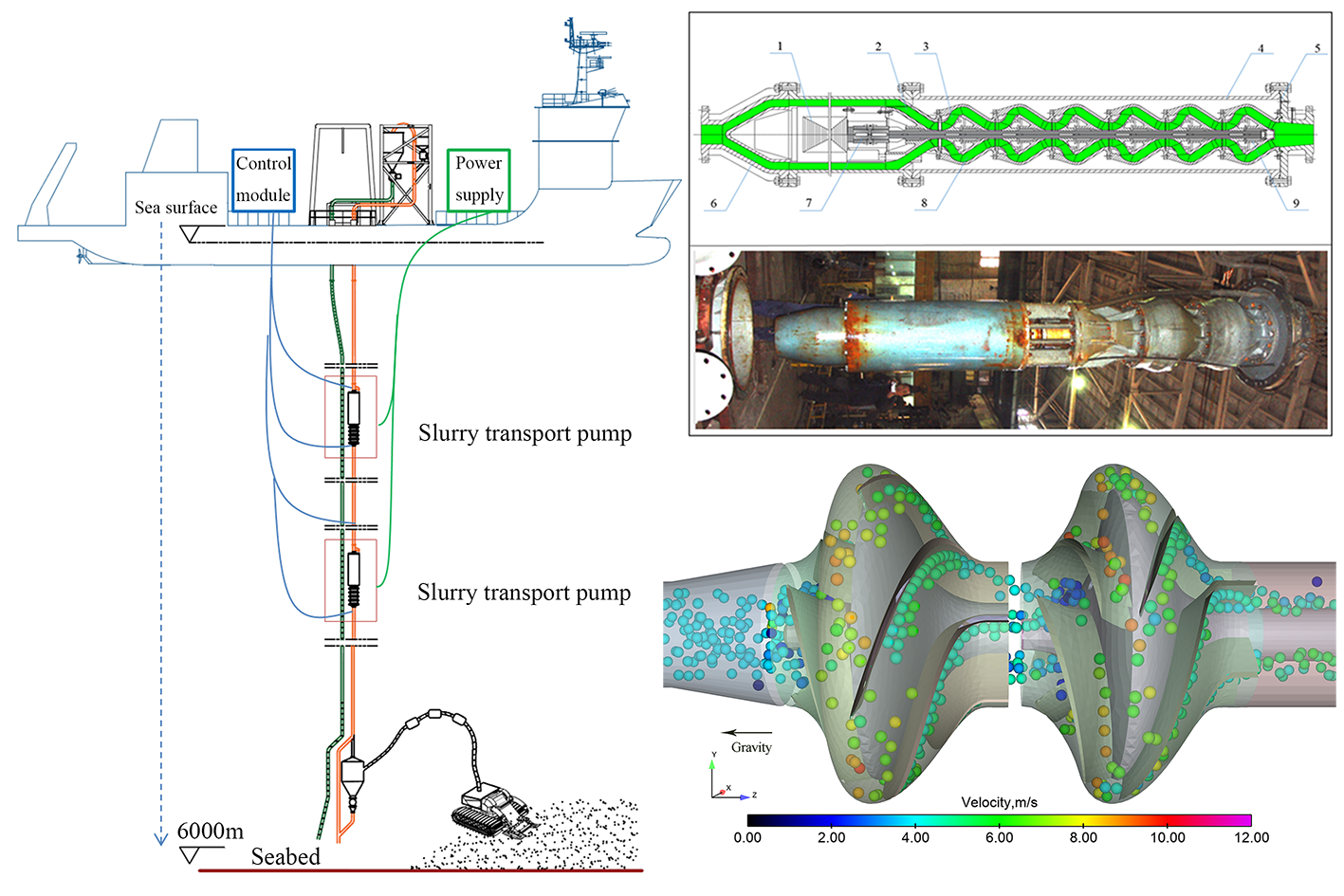
1. Introduction
2. Materials and Methods
2.1. Geometric Model
2.2. Basic Assumptions
2.3. Mathematical Model
2.4. Numerical Method
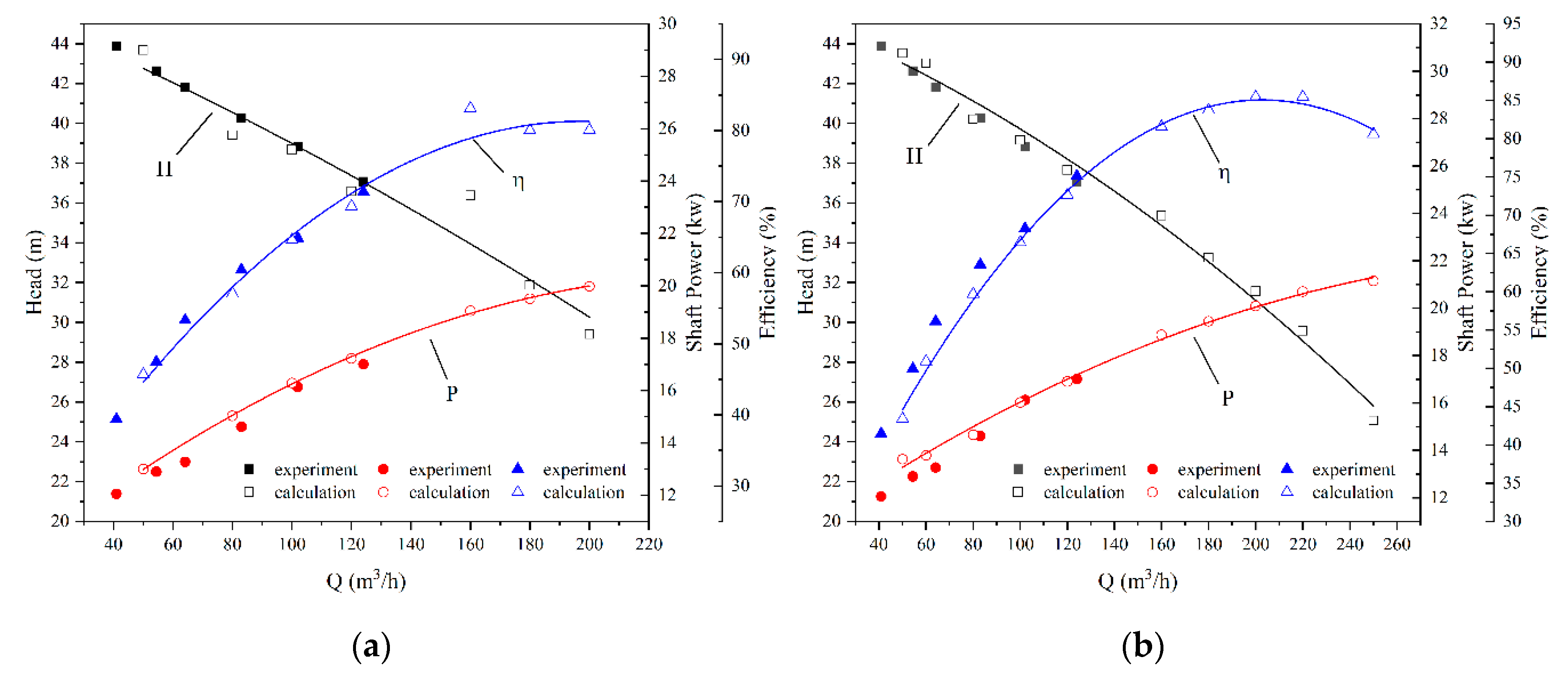
3. Experiment and Validation
3.1. Experimental Device
3.2. Experimental Result
4. Results and Discussion
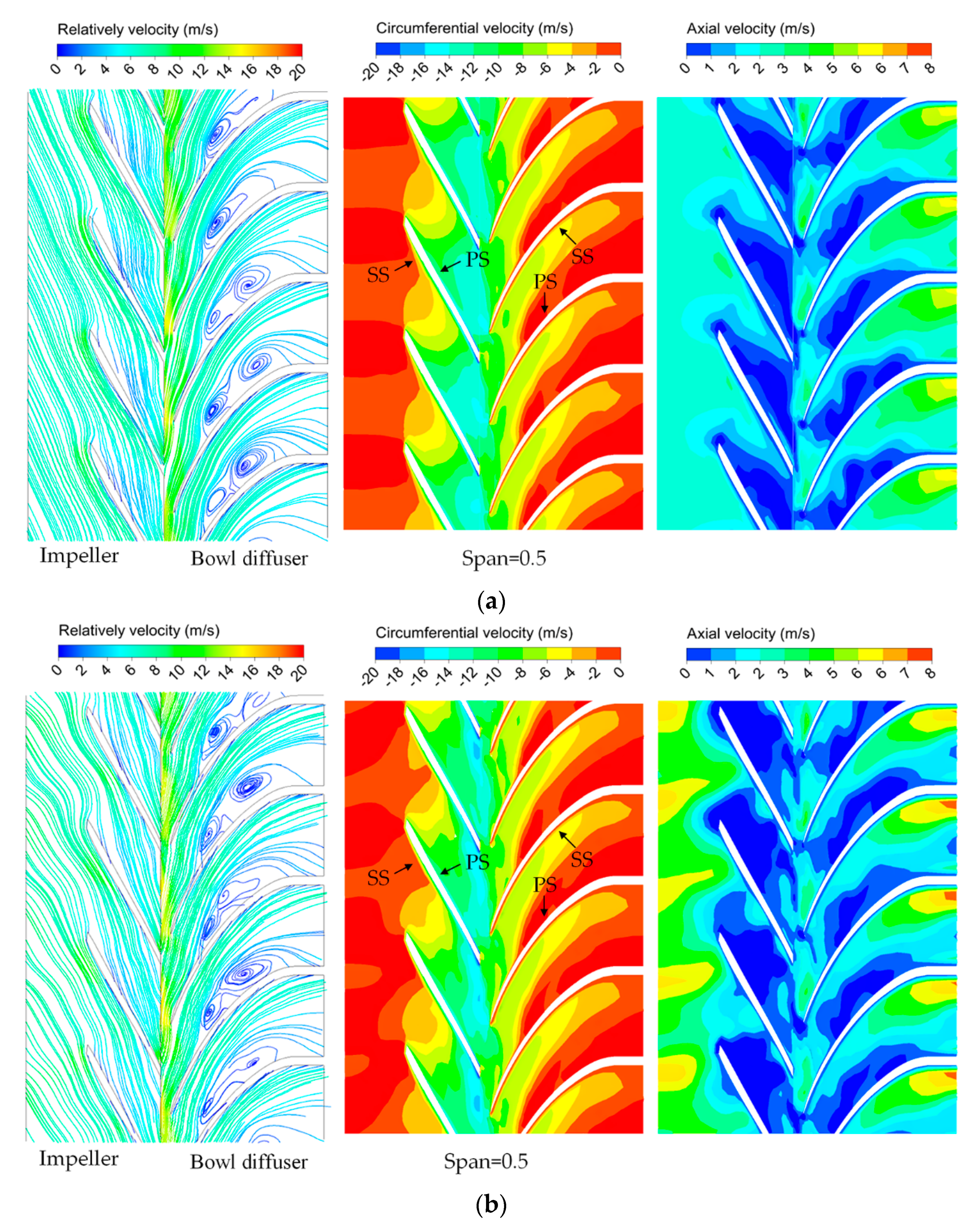
4.1. Flow Features
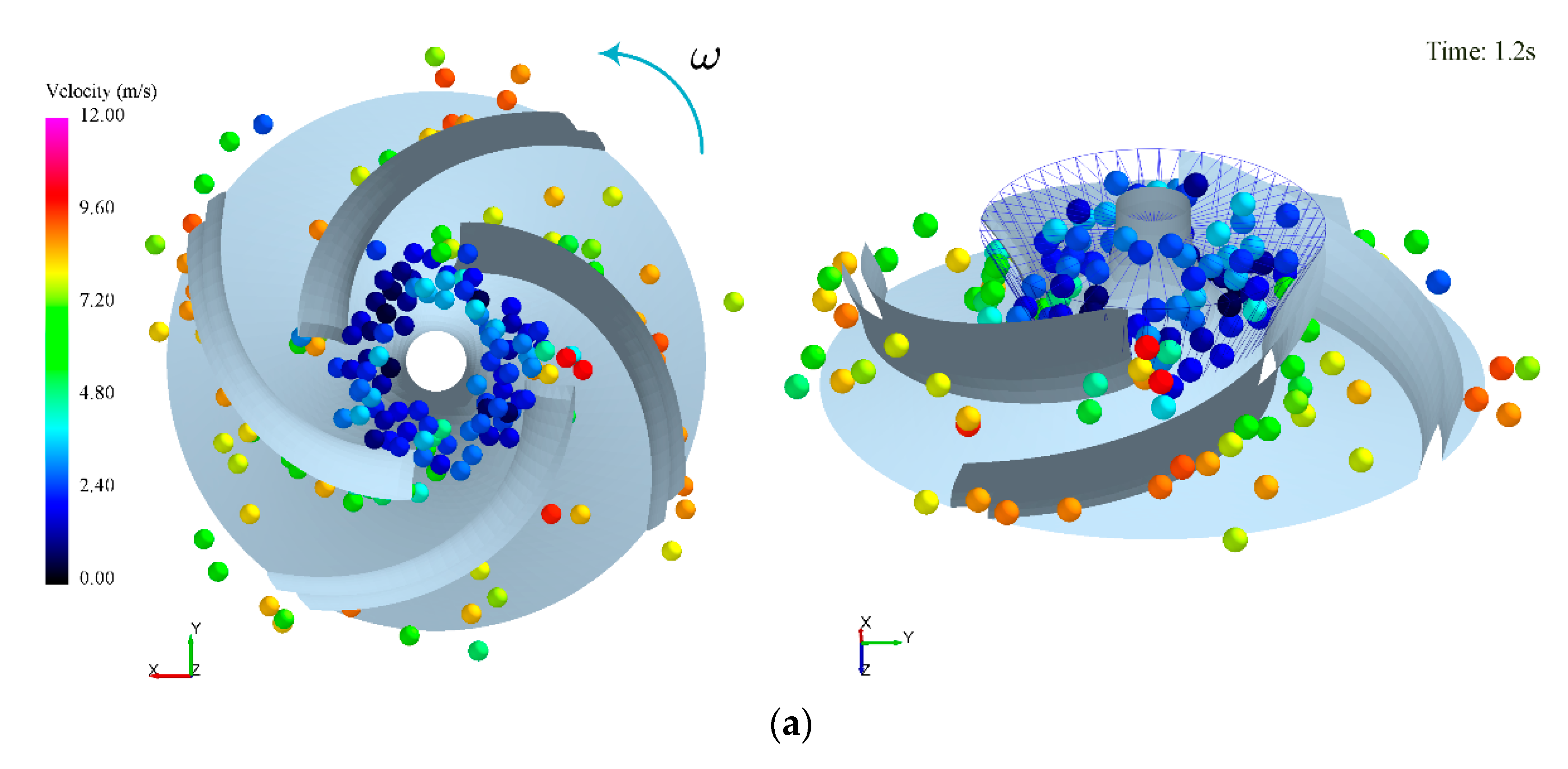
4.2. Distribution and Motion of Patticles
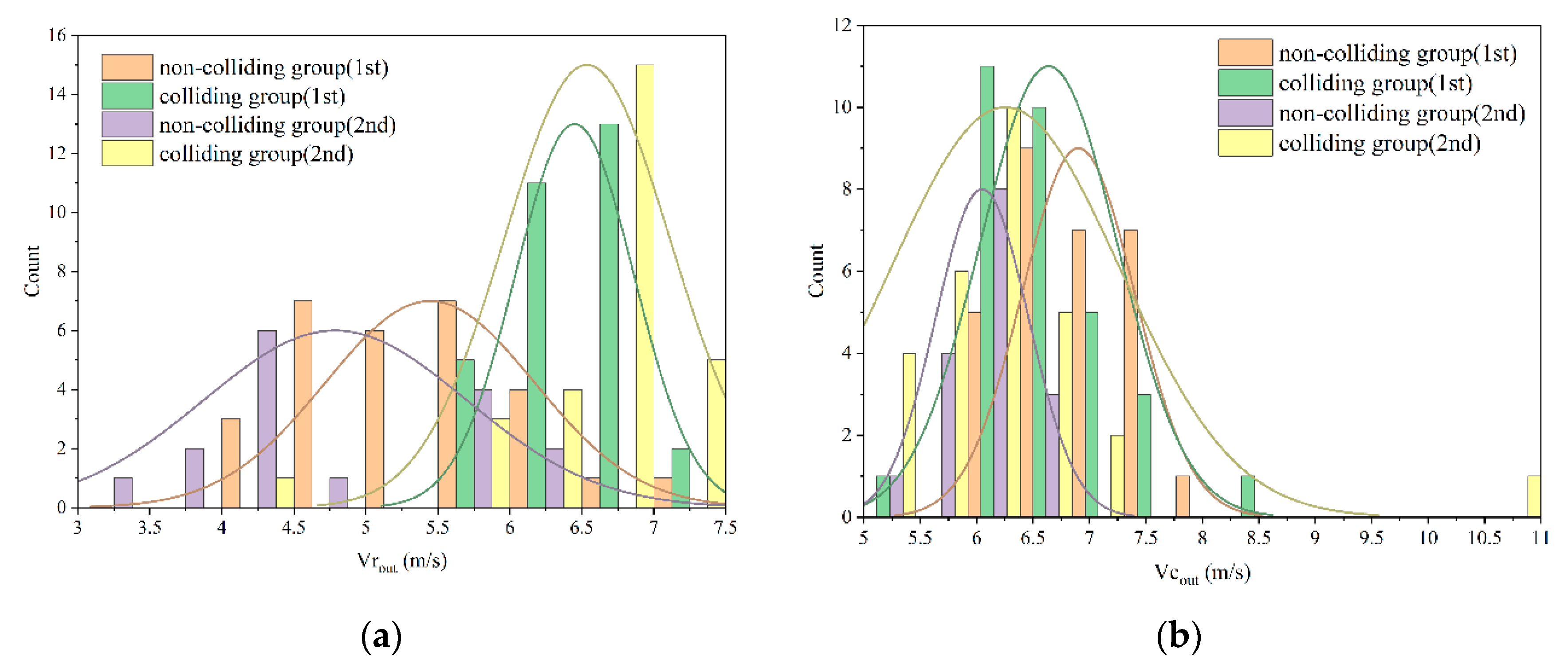
4.2.1. Characteristics of Particle Swarm
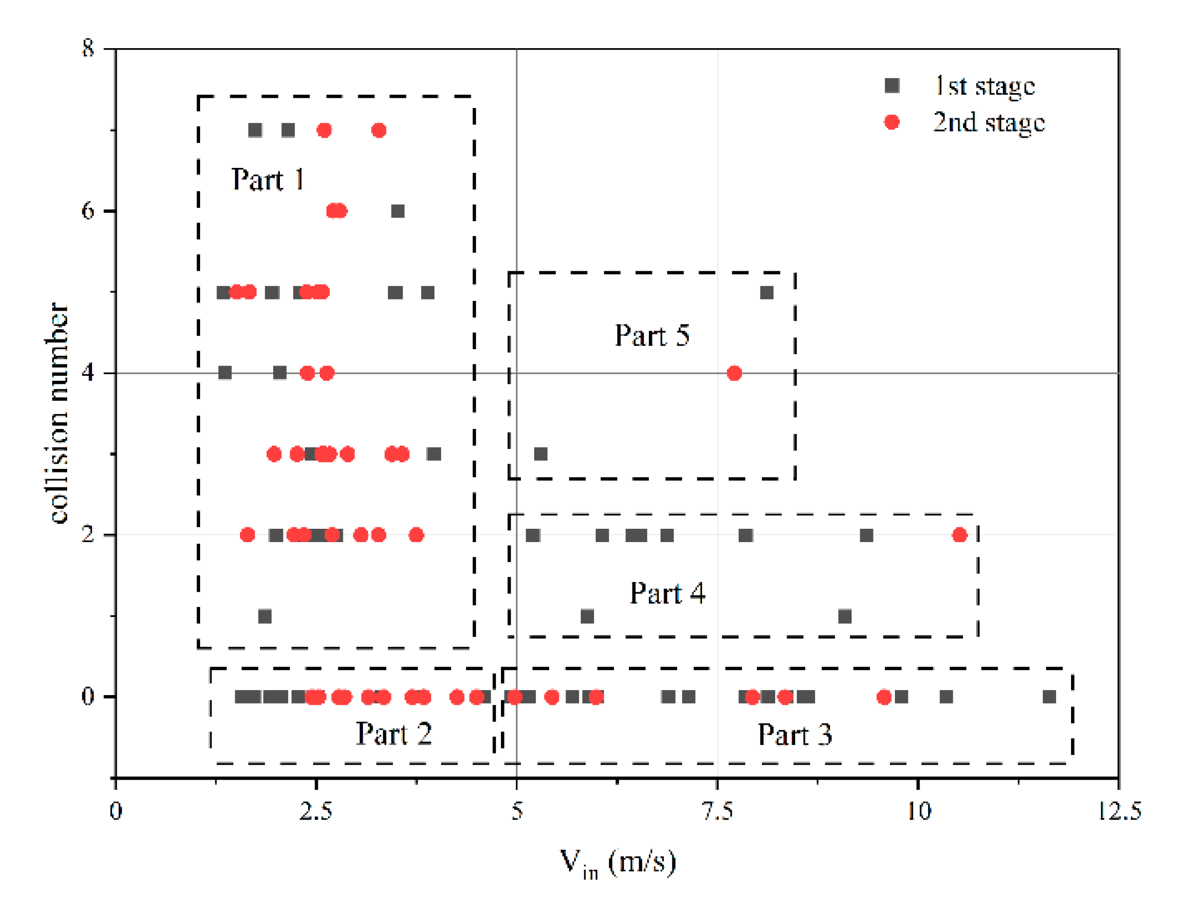
4.2.2. Particle Motion in Impeller
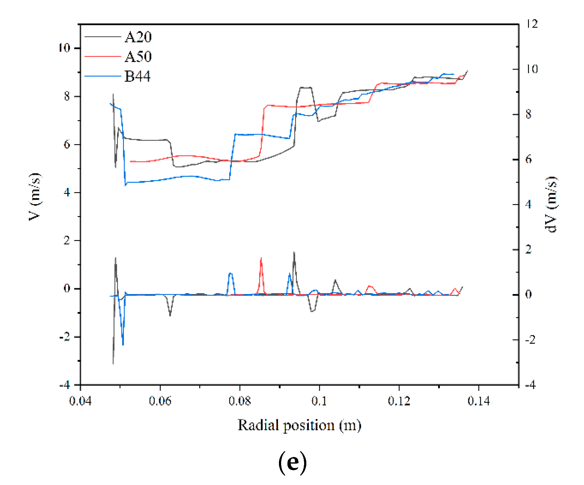
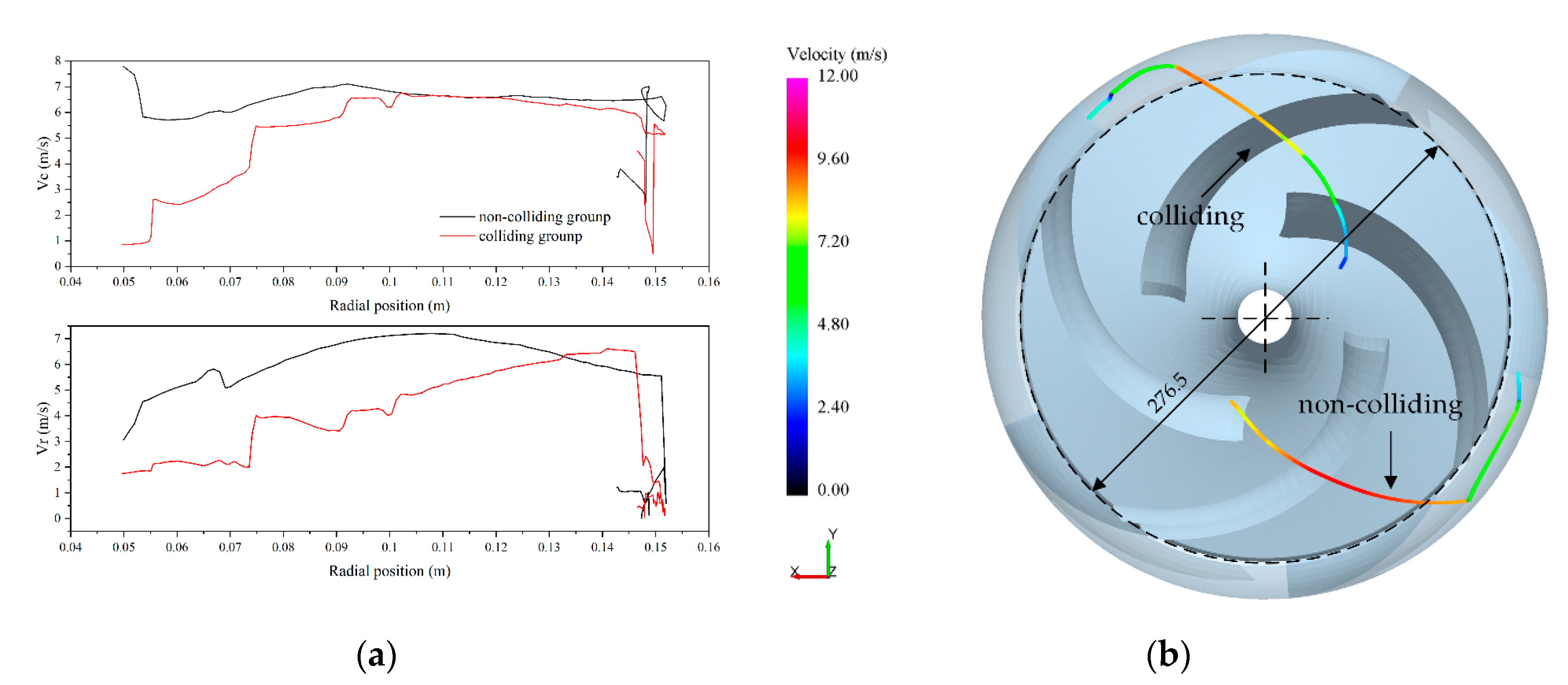
4.2.3. Particle Motion in Bowl Diffuser
5. Conclusions
Author Contributions
Funding
Conflicts of Interest
References
- Hein, J.R.; Mizell, K.; Koschinsky, A.; Conrad, T.A. Deep-ocean mineral deposits as a source of critical metals for high- and green-technology applications: Comparison with land-based resources. Ore Geol. Rev. 2013, 51, 1–14. [Google Scholar] [CrossRef]
- Glasby, G.P.; Li, J.; Sun, Z. Deep-Sea Nodules and Co-rich Mn Crusts. Mar. GeoResour. Geotechnol. 2014, 33, 72–78. [Google Scholar] [CrossRef]
- Sharma, R. Environmental Issues of Deep-Sea Mining. Procedia Earth Planet. Sci. 2015, 11, 204–211. [Google Scholar] [CrossRef]
- Frimanslund, E.K.T. Feasibility of Deep-Sea Mining Operation within Norwegian Jurisdiction. Master’s Thesis, Norwegian University of Science and Technology, Trondheim, Norwegian, 2016. [Google Scholar]
- Deepak, C.R.; Shajahan, M.A.; Atmanand, M.A.; Annamalai, K.; Jeyamani, R.; Ravindran, M.; Schulte, E.; Handschuh, R.; Panthel, J.; Grebe, H.; et al. Developmental Tests On the Underwater Mining System Using Flexible Riser Concept. In Proceedings of the Fourth ISOPE Ocean Mining Symposium, Szczecin, Poland, 23–27 September 2001. [Google Scholar]
- Pougatch, K.; Salcudean, M. Numerical modelling of deep sea air-lift. Ocean Eng. 2008, 35, 1173–1182. [Google Scholar] [CrossRef]
- Liu, S.; Yang, N.; Han, Q. Research and development of deep sea mining technology in China. Proc. Int. Conf. Offshore Mech. Arct. Eng. OMAE 2010, 3, 163–169. [Google Scholar] [CrossRef]
- Kurushima, M.; Kuriyagawa, M.; Koyama, N.K. Japanese Program for Ikp Seabed Mineral Resources DeveIopmen. In Proceedings of the Offshore Technology Conference, Houston, TX, USA, 1–4 May 1995. [Google Scholar] [CrossRef]
- Zou, W. COMRA’s research on lifting motor pump. In Proceedings of the Seventh ISOPE Ocean Mining Symposium, Lisbon, Portugal, 1–6 July 2007; pp. 177–180. [Google Scholar]
- Chung, J.S. An articulated pipe-miner system with thrust control for deep-ocean crust mining. Mar. GeoResour. Geotechnol. 1998, 16, 253–271. [Google Scholar] [CrossRef]
- Liu, S.-J.; Wen, H.; Zou, W.-S.; Hu, X.-Z.; Dong, Z. Deep-Sea Mining Pump Wear Prediction Using Numerical Two-Phase Flow Simulation. In Proceedings of the 2019 International Conference on Intelligent Transportation, Big Data & Smart City (ICITBS), Changsha, China, 12–13 January 2019; pp. 630–636. [Google Scholar]
- Cader, T.; Masbernat, O.; Roco, M.C. LDV Measurements in a Centrifugal Slurry Pump: Water and Dilute Slurry Flows. J. Fluids Eng. 1992, 114, 606–615. [Google Scholar] [CrossRef]
- Cader, T.; Masbernat, O.; Roco, M.C. Two-Phase Velocity Distributions and Overall Performance of a Centrifugal Slurry Pump. J. Fluids Eng. 1994, 116, 316–323. [Google Scholar] [CrossRef]
- Shi, B.; Wei, J.J.; Zhang, Y. Phase discrimination and a high accuracy algorithm for PIV image processing of particle–fluid two-phase flow inside high-speed rotating centrifugal slurry pump. Flow Meas. Instrum. 2015, 45, 93–104. [Google Scholar] [CrossRef]
- Shi, B.; Wei, J.; Zhang, Y. A novel experimental facility for measuring internal flow of Solid-liquid two-phase flow in a centrifugal pump by PIV. Int. J. Multiph. Flow 2017, 89, 266–276. [Google Scholar] [CrossRef]
- Kadambi, J.R.; Charoenngam, P.; Subramanian, A.; Wernet, M.P.; Sankovic, J.M.; Addie, G.; Courtwright, R. Investigations of Particle Velocities in a Slurry Pump Using PIV: Part 1, The Tongue and Adjacent Channel Flow. J. Energy Resour. Technol. 2004, 126, 271–278. [Google Scholar] [CrossRef]
- Jialiang, X.; Zhang, H.; Lin, Z.; He, Z.; Xiang, J.; Su, X. Relationship between wear formation and large-particle motion in a pipe bend. R. Soc. Open Sci. 2019, 6, 181254. [Google Scholar] [CrossRef]
- Tarodiya, R.; Gandhi, B.K. Numerical simulation of a centrifugal slurry pump handling solid-liquid mixture: Effect of solids on flow field and performance. Adv. Powder Technol. 2019, 30, 2225–2239. [Google Scholar] [CrossRef]
- Zhu, H.; Zhu, J.; Rutter, R.; Zhang, H.-Q. A Numerical Study on Erosion Model Selection and Effect of Pump Type and Sand Characters in Electrical Submersible Pumps by Sandy Flow. J. Energy Resour. Technol. 2019, 141, 1–58. [Google Scholar] [CrossRef]
- Huang, S.; Su, X.; Qiu, G. Transient numerical simulation for solid-liquid flow in a centrifugal pump by DEM-CFD coupling. Eng. Appl. Comput. Fluid Mech. 2015, 9, 411–418. [Google Scholar] [CrossRef]
- Ndimande, C.; Cleary, P.; Mainza, A.; Sinnott, M. Using two-way coupled DEM-SPH to model an industrial scale Stirred Media Detritor. Miner. Eng. 2019, 137, 259–276. [Google Scholar] [CrossRef]
- Chu, K.; Yu, A. Numerical Simulation of the Gas−Solid Flow in Three-Dimensional Pneumatic Conveying Bends. Ind. Eng. Chem. Res. 2008, 47, 7058–7071. [Google Scholar] [CrossRef]
- Xiao, H.; Sun, J. Algorithms in a Robust Hybrid CFD-DEM Solver for Particle-Laden Flows. Commun. Comput. Phys. 2011, 9, 297–323. [Google Scholar] [CrossRef]
- Gosman, A.D.; Loannides, E. Aspects of Computer Simulation of Liquid-Fueled Combustors. J. Energy 1983, 7, 482–490. [Google Scholar] [CrossRef]
- Morsi, S.A.; Alexander, A.J. An investigation of particle trajectories in two-phase flow systems. J. Fluid Mech. 1972, 55, 193–208. [Google Scholar] [CrossRef]
- Zhou, M.; Wang, S.; Kuang, S.; Luo, K.; Xing, J.; Yu, A. CFD-DEM modelling of hydraulic conveying of solid particles in a vertical pipe. Powder Technol. 2019, 354, 893–905. [Google Scholar] [CrossRef]
- Liu, D.; Fu, X.; Wang, G. Volume fraction allocation using characteristic points for coupled CFD-DEM calculation. J. Tsinghua Univ. Technol. 2017, 57, 720. [Google Scholar] [CrossRef]
- Kang, Y.; Liu, S.; Zou, W.; Zhao, H.; Hu, X.-Z. Design and analysis of an innovative deep-sea lifting motor pump. Appl. Ocean Res. 2019, 82, 22–31. [Google Scholar] [CrossRef]
- Kuntz, G. Advantages of Submersible Motor Pumps in Deep-Sea Mining. J. Pet. Technol. 1980, 32, 2241–2246. [Google Scholar] [CrossRef]


| Impeller | Value | Bowl Diffuser | Value |
|---|---|---|---|
| Inlet diameter (mm) | 135 | Inlet diameter (mm) | 276 |
| Outlet diameter (mm) | 272 | Inlet width (mm) | 26 |
| Blade number | 4 | Blade number | 5 |
| Wrap angle (°) | 111~115 | Wrap angle (°) | 118 |
| Outlet angle (°) | 24 | Outlet angle (°) | 25 |
| Inlet angle (°) | 26 | Inlet angle (°) | 90 |
| Parameters | unit | Test Pump | Prototype Pump |
|---|---|---|---|
| Design flow rate (Q) | 120 | 420 | |
| Design head (H) | m | 40 | 270 |
| Rotating speed (n) | rpm | 1450 | 1450 |
| Specific speed 1 () | 102.17 | 102.17 |
| Interaction of Object | Recovery Factor | Coefficient of Static Friction | Coefficient of Rolling Friction |
|---|---|---|---|
| Particle–particle | 0.44 | 0.27 | 0.01 |
| Pump–particle | 0.5 | 0.15 | 0.01 |
| Grid Number | Cell | Head (m) | Efficiency (%) | ||
|---|---|---|---|---|---|
| 1 | 484,378 | 37.656 | 4.60 | 71.418 | 4.95 |
| 2 | 621,314 | 37.757 | 4.88 | 72.130 | 4.00 |
| 3 | 722,614 | 37.659 | 4.61 | 72.678 | 3.27 |
| 4 | 819,244 | 37.506 | 4.18 | 71.738 | 4.53 |
| Experiment | 36 | 75.138 |
Publisher’s Note: MDPI stays neutral with regard to jurisdictional claims in published maps and institutional affiliations. |
© 2020 by the authors. Licensee MDPI, Basel, Switzerland. This article is an open access article distributed under the terms and conditions of the Creative Commons Attribution (CC BY) license (http://creativecommons.org/licenses/by/4.0/).
Share and Cite
Su, X.; Tang, Z.; Li, Y.; Zhu, Z.; Mianowicz, K.; Balaz, P. Research of Particle Motion in a Two-Stage Slurry Transport Pump for Deep-Ocean Mining by the CFD-DEM Method. Energies 2020, 13, 6711. https://doi.org/10.3390/en13246711
Su X, Tang Z, Li Y, Zhu Z, Mianowicz K, Balaz P. Research of Particle Motion in a Two-Stage Slurry Transport Pump for Deep-Ocean Mining by the CFD-DEM Method. Energies. 2020; 13(24):6711. https://doi.org/10.3390/en13246711
Chicago/Turabian StyleSu, Xianghui, Zhenji Tang, Yi Li, Zuchao Zhu, Kamila Mianowicz, and Peter Balaz. 2020. "Research of Particle Motion in a Two-Stage Slurry Transport Pump for Deep-Ocean Mining by the CFD-DEM Method" Energies 13, no. 24: 6711. https://doi.org/10.3390/en13246711
APA StyleSu, X., Tang, Z., Li, Y., Zhu, Z., Mianowicz, K., & Balaz, P. (2020). Research of Particle Motion in a Two-Stage Slurry Transport Pump for Deep-Ocean Mining by the CFD-DEM Method. Energies, 13(24), 6711. https://doi.org/10.3390/en13246711