Short-Term Forecasting of Large-Scale Clouds Impact on Downwelling Surface Solar Irradiation

Abstract

This study focuses on the use of cloud motion vectors (CMV) and fast radiative transfer models (FRTM) in the prospect of forecasting downwelling surface solar irradiation (DSSI). Using near-real-time cloud optical thickness (COT) data derived from multispectral images from the spinning enhanced visible and infrared imager (SEVIRI) onboard the Meteosat second generation (MSG) satellite, we introduce a novel short-term forecasting system (3 h ahead) that is capable of calculating solar energy in large-scale (1.5 million-pixel area covering Europe and North Africa) and in high spatial (5 km over nadir) and temporal resolution (15 min intervals). For the operational implementation of such a big data computing architecture (20 million simulations in less than a minute), we exploit a synergy of high-performance computing and deterministic image processing technologies (dense optical flow estimation). The impact of clouds forecasting uncertainty on DSSI was quantified in terms of cloud modification factor (CMF), for all-sky and clear sky conditions, for more generalized results. The forecast accuracy was evaluated against the real COT and CMF images under different cloud movement patterns, and the correlation was found to range from 0.9 to 0.5 for 15 min and 3 h ahead, respectively. The CMV forecast variability revealed an overall DSSI uncertainty in the range 18–34% under consecutive alternations of cloud presence, highlighting the ability of the proposed system to follow the cloud movement in opposition to the baseline persistent forecasting, which considers the effects of topocentric sun path on DSSI but keeps the clouds in “fixed” positions, and which presented an overall uncertainty of 30–43%. The proposed system aims to support the distributed solar plant energy production management, as well as electricity handling entities and smart grid operations.

1. Introduction

Over the last decades, the main goal for worldwide sustainable development and mitigation policies for climate change is the turn to renewables against coal energy production. According to the recent five-year forecasts report of the International Energy Agency (IEA) [1], until 2024, renewable energy production is designated to increase by 50%, with solar PV capacity leading this increment by more than half of this increase globally (~60%). Accurate knowledge of solar resources with their temporal and spatial variability is a prerequisite for every solar energy technology and for the integration of solar energy exploitation systems in every country’s share of annual electricity generation [2]. Forecasting of solar plant output is a powerful operational tool during solar energy systems deployment [3]. Based on the solar radiation attenuation potential, the key atmospheric parameter governing the amount of solar irradiance reaching the earth’s surface is cloud coverage, and the challenge for solar resources forecasting is the prediction of the future position and optical properties of clouds, which shows great spatial and temporal variability.

Forecasting solar irradiance techniques vary with the forecasting horizon depending on the observation methods (in situ sensors, spaceborne sensors, numerical weather prediction (NWP), etc.) that are considered in order to be suitable to the specific needs of their different applications (energy system optimization, energy trading, dispatch). A review of these methods provided by several studies [4,5].

The aim of this study is the short–term solar forecasting (a few minutes up to 3 h ahead). A well-established operational technique to predict future cloud location is based on the use of cloud motion vectors (CMVs). This method is valid under the assumptions of simple horizontal advection of cloud formations, under constant speed and their rather stable shape and brightness [6]. This assumption of persistency of these attributes could be considered near-real only for small time periods (up to a few hours). The CMVs are calculated by matching cloud in consecutive cloud images, provided either from satellites or ground-based sky cameras, and assuming constant cloud speed, the prediction of future clouds is performed applying CMVs to the latest cloud image. Although CMVs were introduced together with the launch of the first meteorological satellites [7], they are used as an operational tool to weather nowcasting and wind field retrieval inside the atmosphere [8], but also in short-term solar forecasting from the late 90 s [9]. The early stages of the CMV method for solar irradiance forecasting are described by these groups [4,6,10], with the major development of satellite-based methods taking place in the first decade of the new century [11,12,13]. On the other hand, over the last decade, the use of sky cameras has become more common for estimating CMV [14,15], providing forecasts at a local scale.

Several approaches for cloud prediction using CMVs to obtain forecasts of solar irradiance have been proposed through all of these years. Chow et al. [16] applied a cross-correlation method to two consecutive sky images partitioned into subsets of pixels in order to derive CMVs. Using the global vector determined from the two previous images advected the cloud map in order to forecast cloud cover up to 5 min ahead. Wang et al. [17] derived CMVs using the block-matching method on MSG cloud physical properties and advected those cloud properties 4 h ahead. Using the cloud physical properties of the surface insolation under clear and cloudy skies derived from SEVIRI imagery (CPP-SICCS algorithm), DSSI forecasted values were retrieved using the advected cloud properties. Yang et al. [18] derived the CMV field applying particle image velocimetry (PIV) to FY-4A (a complete list of abbreviations can be found in Abbreviations section) satellite cloud images in order to forecast DSSI up to 3 h.

In addition, new approaches to cloud prediction provided by computer vision methods and particularly cloud motion estimation using optical flow techniques. The concept of optical flow estimation is to compute an approximation to the motion field of every pixel (dense optical flow) through the variations of image intensity with time, under the assumption that these variations are solely due to cloud movements. Fleet and Weiss [19] provide several techniques that have been proposed for gradient-based optical flow estimation. In the last decade, some effort had been putting into predicting cloud motion using optical flow techniques in the context of solar forecasting. Wood-Bradley et al. [20] tracked and predicted cloud movement in sky images using the optical flow method of Lucas–Kanade [21]. Cros et al. [22] proposed the combination of correlation phase and optical flow methods to extract CMVs from MSG-10 data in order to predict cloud index maps. In addition, they used the already operational block-matching technique and compared the forecasts both among them as well as the persistence approach. They concluded that the optical flow technique outperformed all the other methods with a better computational time. Nonnenmacher et al. [23] selected optical flow among other feature tracks methods and specifically an open-source code of optical flow algorithm provided by Sun et al. [24,25] to calculate CMVs from GEOS satellite-derived cloud index images. The advected clouds translated into irradiance forecast using an improved (ground measurements) semi-empirical satellite-to-irradiance model. Chow et al. [26] using sky images forecasted cloud locations up to 15 min ahead using two methods, variational optical flow (VOF) technique and cross-correlation method (CCM), and by comparing them with image, persistence method found that VOF forecast outperformed the other two methods. Peng et al. [27] summarized and evaluated seven different state-of-the-art sky images cloud motion estimations using optical flow and block-matching approaches and particle image velocimetry and also proposed a hybrid model incorporating the block-matching and optical flow techniques which outperformed the aforementioned individual approaches. Du et al. [28] used the optical flow algorithm proposed by Sun et al. [25] to compute CMVs from sky images. They forecasted solar irradiance using the predicted sky images and irradiance fields calculated by a radiative transfer model under clear sky and overcast conditions. The comparison with in situ irradiance measurements showed that their results outperform the persistence model.

Urbich et al. [29] used an optical flow algorithm (TV-L¹) to forecast satellite-derived effective cloud albedo up to 4 h, and using SPECMAGIC NOW, surface irradiances were calculated. In addition, in the context of short-term forecasting of cloud albedo, a comparison of two optical flow methods TV-L¹ and Farnebäck, was performed, with the first method performing better than the former one. Teerakawanich et al. [30] used the optical flow algorithm proposed by Farnebäck to track cloud movement on sky images and the calculated vectors used as input in a convolution neural network (CNN) in order to predict cloud cover events 1 to 2 min in advance. The method showed better results during wintertime when the clear sky and thick clouds are the prevailing sky conditions. During those days, the prediction error was as good as 5%, with this error increasing in the presence of thin clouds. Li et al. [31] performed cloud tracking and forecasting to satellite images using Shi–Tomasi’s method to select features to track, image filtering and finally Horn and Schunck (HS) and Lucas–Kanade (LK) optical flow method to track those features. Although the optical flow methods used originally are dense, the segmentation performed by Shi–Tomasi’s method resulted in a sparse vector field, which requires less computational time. They found that LK with a Gaussian filter as a preprocessor was the most accurate and efficient method. However, their main finding was that satellite cloud images could be useful for irradiance predictions, providing predictable features in wide areas with long-time movement. In this study, for the calculation of the dense optical flow, the Farnebäck [32] and TV-L¹ [33] algorithms have been implemented using OpenCV open-source library.

For intra-hour solar forecasting, with very high spatial and temporal resolution and for specific locations, ground-based sky-imaging systems provide the cloud conditions for CMV calculations [34]. When the forecasting horizon is increasing, a larger spatial scale of cloud coverage is needed with high temporal resolution; therefore, the extrapolation of future cloud locations is conventionally conducted using CMVs derived from geostationary satellite images [6].

As the aim of the study is the use of CMV techniques for DSSI forecasting up to 3 h, we use satellite data as reference input in order to assess cloud dynamics. The broad spatial coverage and constant area monitoring of geostationary satellite data are useful for the provision of cloud forecasts in high spatial and temporal resolution. In this direction, satellite-derived cloud optical thickness (COT) images and cloud modification factor (CMF) simulated images are used as inputs to the two optical flow algorithms resulting in a number of different experiments. COT maps provided by EUMETSAT SAFNWC [35] and CMF maps were built up using the provided COT and radiative transfer algorithms. The first phase of the validation procedure was conducted using the real values of those parameters, comparing the forecasted with the real COT and CMF values.

The predicted cloud features, along with other variables, are used as inputs to the fast radiative transfer model (FRTM) that was developed and described by Kosmopoulos et al. [36] in order to produce the corresponding DSSI forecasts. As it has been already mentioned, the main target (challenge) of this study is the rapid computational procedures in order to make this tool operationally implementable. To this end, fast calculations of surface solar irradiances must be obtained, with a duration smaller than the time interval of satellite cloud product is renewed (15 min).

For evaluation purposes, we have benchmarked optical flow cloud and irradiance forecasts against the persistence (PRS) approach. PRS is a forecasting choice of keeping the last real value of COT and CMF constant for all the subsequent time steps. The PRS for DSSI was enhanced to incorporate variations due to the topocentric sun path, and the air mass position changes. The main goal of this study is to explore existing approaches in CMV optimized derivations using dense optical flow algorithms in order to predict cloud motion and through rapid calculation procedures of DSSI to produce fast and accurate irradiance forecasts up to 3 h ahead with 15 min increment onto 5 × 5 km grids across Europe and North Africa. Thus, in Section 2, satellite data, the two optical flow algorithms, their implementation to predict COT and CMF maps and DSSI calculations are described. In addition, in the same section, the evaluation techniques and formulas are given. In Section 3, results from four different cloud forecasting experiments are presented and analyzed for three days, characterized by various cloud patterns, speeds and direction change. Additionally, the respective DSSI impact results in terms of CMF are given and discussed. Finally, in Section 4, the conclusions are presented.

2. Materials and Methods

The method we use to produce the DSSI forecast is presented in the following sections. We focus on the cloud-related input to the FRTM method described in Section 2.3.

Input data are obtained from geostationary satellites and used with two different optical flow approaches, the Farnebäck and the TV-L¹ (FRB and TVL hereafter) applied either on COT and on CMF. We select to treat both variables in order to investigate differences in the final product. COT is a satellite-based product that can be directly retrieved in real time without any post-processing. It describes the attenuation of DSSI reaching the surface through a cloud. On the other hand, CMF describes more directly the cloud effect on DSSI (it describes the attenuation as a fraction compared with cloudless sky DSSI) and especially the important variations caused by low COT values. Cloud inputs are then fed to the FRTM to produce the operational forecast.

In order to evaluate the results, 3 days in April 2020 were selected, when different parts of Europe were cloud covered. It consists of 52.2 million individual cases where forecasted results of two CMV (using either COT or CMF) methods are evaluated. The evaluation is focusing on the forecasted CMF or COT (also retrieved as irradiation using the FRTM) compared with the ones that are retrieved based on the “real” satellite images that follow. Hence, it directly focuses on the CMV methodology itself and not on the uncertainties of the satellite-based COT retrievals.

2.1. Clouds Observation

The main earth observation data source used to quantify the clouds’ effect on DSSI is the cloud optical thickness (COT) product of the EUMETSAT’s SAFNWC, retrieved from the Meteosat second generation SEVIRI instrument (MSG/SEVIRI) in near-real time (nowcasting). The retrieval algorithm uses radiances from the 0.6 and 1.6-micron channels, as described in [35]. The COT product uncertainty is related to the MSG/SEVIRI retrieving methodology uncertainty and hence, propagates into the irradiance retrieval, becoming the highest source of errors in the short-term forecasting simulations [37]. The spatial and temporal resolution of the MSG COT is 5 km over nadir and 15 min, respectively, also indicating the moving step for the CMV techniques.

For the calculation of the clouds’ effect on DSSI, we used the cloud modification factor (CMF) for more generalized results and for a better understanding of the overall impact regardless of the climatological conditions. The CMF is described by the following Equation (1):

CMF = DSSI/DSSI_cls,

(1)

where DSSI is the irradiance under actual sky conditions and DSSI_cls is the irradiance under clear sky conditions as simulated by the FRTM [36].

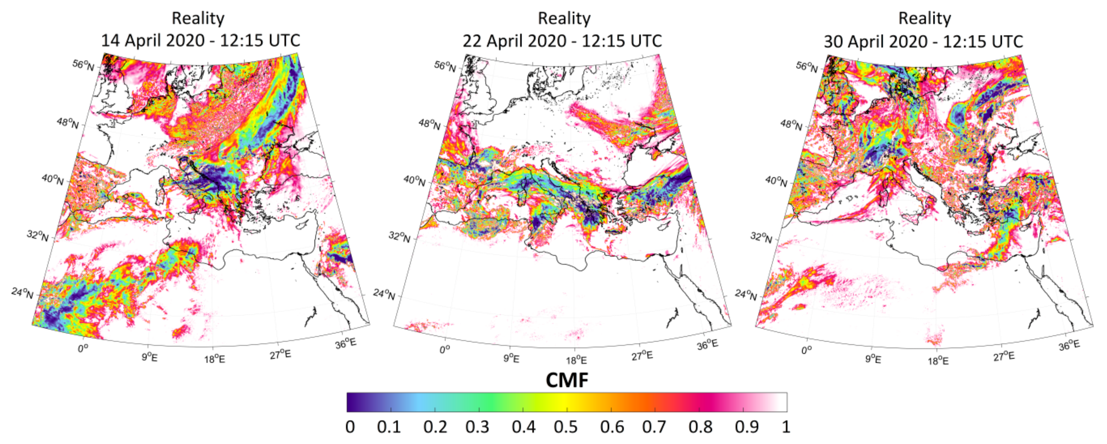
As a result, the CMF takes values between 0 and 1, indicating the clear sky DSSI with 1 (i.e., no cloud effect) and all the lower values characterizing the DSSI under the clouds effect. At the earth’s surface, CMF could appear higher than 1, caused either by the over-irradiance effect [38] or by the misestimation of clear sky DSSI; all these cases are treated as 1 in the algorithm presented here. In this direction, we took 3 different days in terms of cloud patterns and motion speeds to compare the CMV approaches, using COT and CMF, respectively, and see as well their performance against the PRS approach, which is not realistic in a moving atmosphere. Figure 1 shows 14, 22 and 30 April 2020, in terms of CMF at 12:15 UTC. These days present totally different cloud motion patterns in terms of cloud direction change and speed.

Table 1. The cloud motion vector characteristics and statistics of the selected days in terms of average cloud speed (ACS) and cloud direction change (CDC) under all-sky conditions, clear to cloudy and cloudy to clear sky condition transition (TRNs) and cloudy persistence during the studied 3 h time horizon, i.e., from 9:15 to 12:15 UTC.

Cloud Motion Vector Analysis	14/04/2020	22/04/2020	30/04/2020
Total number of data comparison	1.45 million/image × 12 forecasts × 3 days = 52.2 million
Cloud coverage (million pixels)	9.0 (52%)	5.6 (32%)	9.9 (57%)
ACS (km/h)	37	11	23
CDC (degrees)	3	13	7
Total number of clear to cloudy TRN	2.8 (16%)	1.7 (9.7%)	2.5 (14.5%)
ACS (km/h)	49	17	36
CDC (degrees)	6	21	13
Total number of cloudy to clear TRN	1.3 (7.6%)	1.1 (6.2%)	1.0 (5.5%)
ACS (km/h)	42	14	27
CDC (degrees)	2	15	7
Total number of cloudy to cloudy	5.3 (30.3%)	3.0 (17.2%)	6.8 (39%)
ACS (km/h)	20	2	6
CDC (degrees)	1	3	1

presents the cloud motion vector analysis of the selected days focusing on the cloud coverage, the average cloud speed (ACS) and the cloud direction change (CDC) under various sky condition transition (TRN hereafter) patterns, i.e., from clear to cloudy, from cloudy to clear and from cloudy to cloudy. From the total number of the 52.2 million comparison data, which represent the 1.45 million pixels of each image, multiplied by 12, which are the time steps ahead (3 h) for each of the three days, the cloud covered pixels are almost 9 million for 14 April 2020, 5.6 million for 22 April 2020 and 9.9 million for 30 April 2020 during the 3 h time horizon from 9:15 to 12:15 UTC. The ACS and CDC are in the range of 11–37 and 3–13, respectively, indicating the wide range of different comparison conditions. The corresponding ACS for the clear to cloudy, cloudy to clear and cloudy to cloudy TRNs are in the range of 17–49, 14–42 and 2–20, respectively, while the CDC ranges for the same TRN categories are 6–21, 2–15 and 1–3, respectively. The aforementioned cloud pattern characteristics indicate a large number of comparison data (17.4 million pixels/day), covering a wide range of cloud coverage, ACS and CDC, and hence, highlight the comparison logic and principles that this study followed. Additional days would be helpful in terms of the result statistics, but the number of points analyzed here for various ranges of ACS and CDC (Table 1) is already very high, as a result of the high pixel resolution, the extend of the domain and the fact that in such a large domain 3 h of cloud movement cannot be considered homogeneous.

2.2. Cloud Motion Vector

In this study, we obtain CMVs in order to predict the motion of the clouds by applying computer vision techniques and particularly calculating the optical flow displacement vectors between two images of satellite-derived cloud-related parameters, COT and CMF, by assuming that cloud’s displacements are two dimensional (image plane). During our analysis, two different computer vision algorithms to forecast cloudiness using optical flow were implemented, the FRB method and the TVL method.

The innovation of the study relies on the implementation of two state-of-the-art methods of computer vision to obtain optical flow using COT and CMF images in order to calculate CMVs and forecasting cloudiness. These cloud-related parameters were used for the first time as inputs for calculating optical flow in order to investigate the impact on the accuracy of the results, given the differences in the nature of these cloud-related inputs as described in the previous section. In addition, the algorithm parameters that provide the best results for both algorithms were determined through different experimental setups. We benchmarked these two methods against the PRS approach, which assumes that the motion of the clouds is inexistent and only the other parameters change.

2.2.1. Optical Flow

Optical flow is the apparent motion of objects between consecutive frames, caused by the relative movement between the object and camera. Onto the two-dimensional image plane, the optical flow displacement vectors can be considered as the projection of real three-dimensional motion vectors of an object [19]. The problem of optical flow estimation is outlined as the approximation of the motion field from image intensity variations with time, solely attributed to objects displacement. A number of different approaches to motion estimation have been proposed through the years, and in the context of the current study, the gradient-based approaches of optical flow estimation [19] are utilized. The starting point for optical flow estimation is that the image intensity I(x,y,t) satisfies the following equation:

$$\mathrm{I}\left(\mathrm{x},\mathrm{y},\mathrm{t}\right)=\mathrm{I}\left(\mathrm{x}+\mathrm{dx}, \mathrm{y}+\mathrm{dy}, \mathrm{t}+\mathrm{dt}\right)$$

(2)

where for an infinitesimal time interval, dt, dx and dy are the horizontal and vertical displacements of an image region (pixel). This equation formulates the basic hypothesis of optical flow estimation methods, the assumption of brightness constancy, namely the intensity of the pixels of an object can be considered constant for consecutive images. By taking Taylor’s series expansion of the right part of Equation (2) and truncating second and higher-order terms, the optical flow constraint equation is obtained:

$$\frac{\partial \mathrm{I}}{\partial \mathrm{x}}\frac{\mathrm{dx}}{\mathrm{dt}}+\frac{\partial \mathrm{I}}{\partial \mathrm{y}}\frac{\mathrm{dy}}{\mathrm{dt}}+\frac{\partial \mathrm{I}}{\partial \mathrm{t}}=0\iff \overrightarrow{\nabla }\mathrm{I}·\overrightarrow{\mathrm{u}}+\frac{\partial \mathrm{I}}{\partial \mathrm{t}}=0$$

(3)

where $\overrightarrow{\mathrm{u}}\equiv {\left(\frac{\mathrm{dx}}{\mathrm{dt}},\frac{\mathrm{dy}}{\mathrm{dt}}\right)}^{\mathrm{T}}={\left({\mathrm{u}}_1,{\mathrm{u}}_2\right)}^{\mathrm{T}}$ is the velocity field or just the optical flow. As long as the horizontal and vertical image gradients and time gradient of image intensity are known, this equation has two unknown variables u₁ and u₂, so it cannot be solved, and in order to obtain the solution of Equation (3), an additional constrain can provide the other equation needed.

For this study, in order to calculate the optical flow of cloud fields, we focused on two well-established differential methods of estimating optical flow, and they differ only in the mathematical techniques obtaining the solutions. The first algorithm provided by Farnebäck [32] (FRB) is a two-frame motion estimation technique based on polynomial expansion in the neighborhood of each pixel. TVL [33] is the second algorithm utilized in this study for optical flow estimation, which is an efficient numerical scheme and implements the optical flow estimation method introduced by Zach et al. [39], based on the minimization of a function containing a data term using the L¹ norm and a regularization term using the total variation of the flow. In the bibliography of the aforementioned methods, both algorithms were evaluated on a widely used test sequence with known velocity filed, the Yosemite sequence of images, and FRB and TVL methods had small average angular error compared to other techniques [32,33].

Both optical flow estimation methods, FRB and TVL, were used in order to calculate CMVs using as input COT and CMF images. Since the optical flow algorithms accept only 8-bit grayscale images (i.e., 0–255 value range), the real COT and CMF values were assigned to the grayscale values. For the CMF values, this assignment was performed with a one-by-one formula, while for the modification of COT, a different formula was applied. Since the effective COT values that directly interact with the DSSI and cause a significant variation of the CMF are in the range 0–3 of COT, the digitization and extrapolation of this small part of the COT range to a wider grayscale values range was necessary, in order the optical flow algorithms to work properly. To this direction, instead of making the one-by-one assignment of COT values to 0–255 grayscale, Equation (4) was applied to COT values in order to take denser bins of grayscale values in the 0–3 COT range.

$$\mathrm{f}\left(\mathrm{x}\right)=\sqrt[8]{{128}^8\mathrm{x}}, \mathrm{for} \mathrm{x}\ge 0$$

(4)

Once the CMVs are calculated, the next step is to forecast cloudiness in terms of COT and CMF, based on this motion field. Initially, two consecutive images of COT and CMF were used as input to both optical flow algorithms (FRB and TVL) in order to derive the CMV field. Then, the calculated CMVs are applied to the last COT or CMF image resulting in the forecasting of the next image. This procedure was repeated for the next 12 time steps in order to reach the 3 h-ahead forecasting horizon. Finally, the forecasted images of COT and CMF, using the inverse functions of those applied in the beginning, were transformed to maps of COT and CMF in their original range of values.

2.2.2. FRB

The FRB method [32] first approximates the variation of the intensity in the neighborhood of every pixel of both frames by quadratic polynomials (the local signal model), by polynomial expansion signal transformation, which is a local coordinate system (x = (x,y)^T) are expressed as:

$$\mathrm{f}\left(x\right)~x^{\mathrm{T}}\mathrm{A}x+{\mathrm{b}}^{\mathrm{T}}x+\mathrm{c}$$

(5)

where the polynomial coefficients (symmetric matrix A, vector b and scalar value c) are estimated by weighted least-squares, fit to the signal values in neighborhood pixels, then, the displacement fields can be estimated by the polynomial expansion coefficients if polynomials undergo an ideal translation and a new signal is constructed assuming a global displacement d. This global displacement is replaced with a spatially varying displacement field d(x), which is the desirable field; if local polynomial approximations are used instead of global and after a series of approximations and parameterizations, a robust algorithm is provided, described by [32] in detail. One of the basic assumptions of the FRB method is that the displacement field is slowly varying in space in order to implement the method over the wider areas than point-wise, which is too noisy. In addition, the FRB method works well with small displacements, in contrast to large displacements, which introduce errors in the model. Using iterations and a priori displacement field in the first step is one-way to obtain more accurate results, and especially the approach of multiscaled displacement estimation can obtain increasingly more accurate estimates starting from a coarse scale to get the first estimate of the displacement field and propagate this through finer scales.

The implementation of the FRB algorithm was made using the functions of OpenCV [40]. The main function of implementing the FRB algorithm takes as input two consecutive frames and returns the computed flow image. Additionally, 8 input parameters must be determined related to the form, and the assumptions of the algorithm and a detailed description of those parameters are given on the OpenCV website [40]. Indicatively, five input parameters determine the pyramidal approach of the method, two are related to the polynomial expansion in each pixel and, finally, operation flags that must do with the a priori displacement field and smoothing filter of the optical flow estimation.

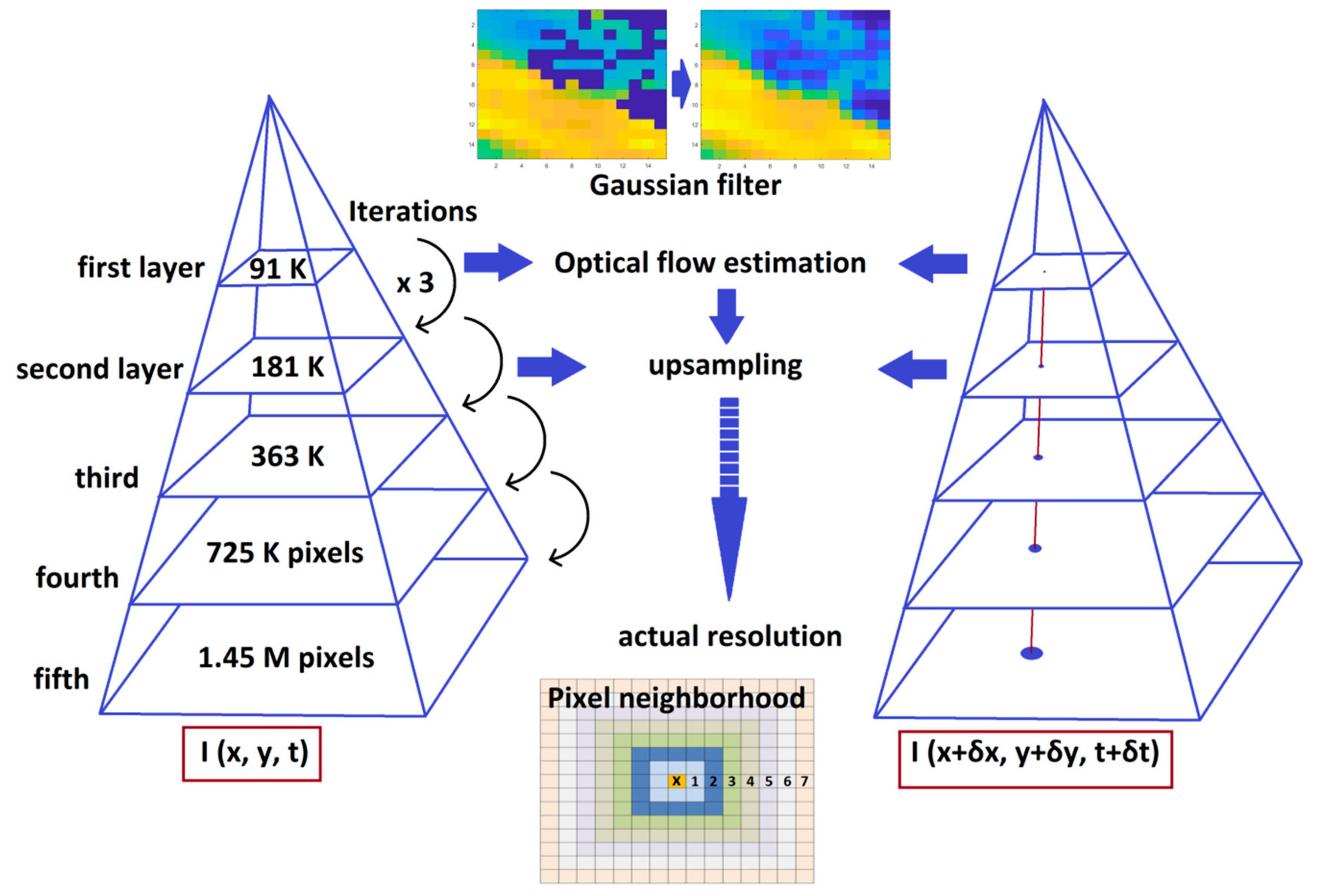
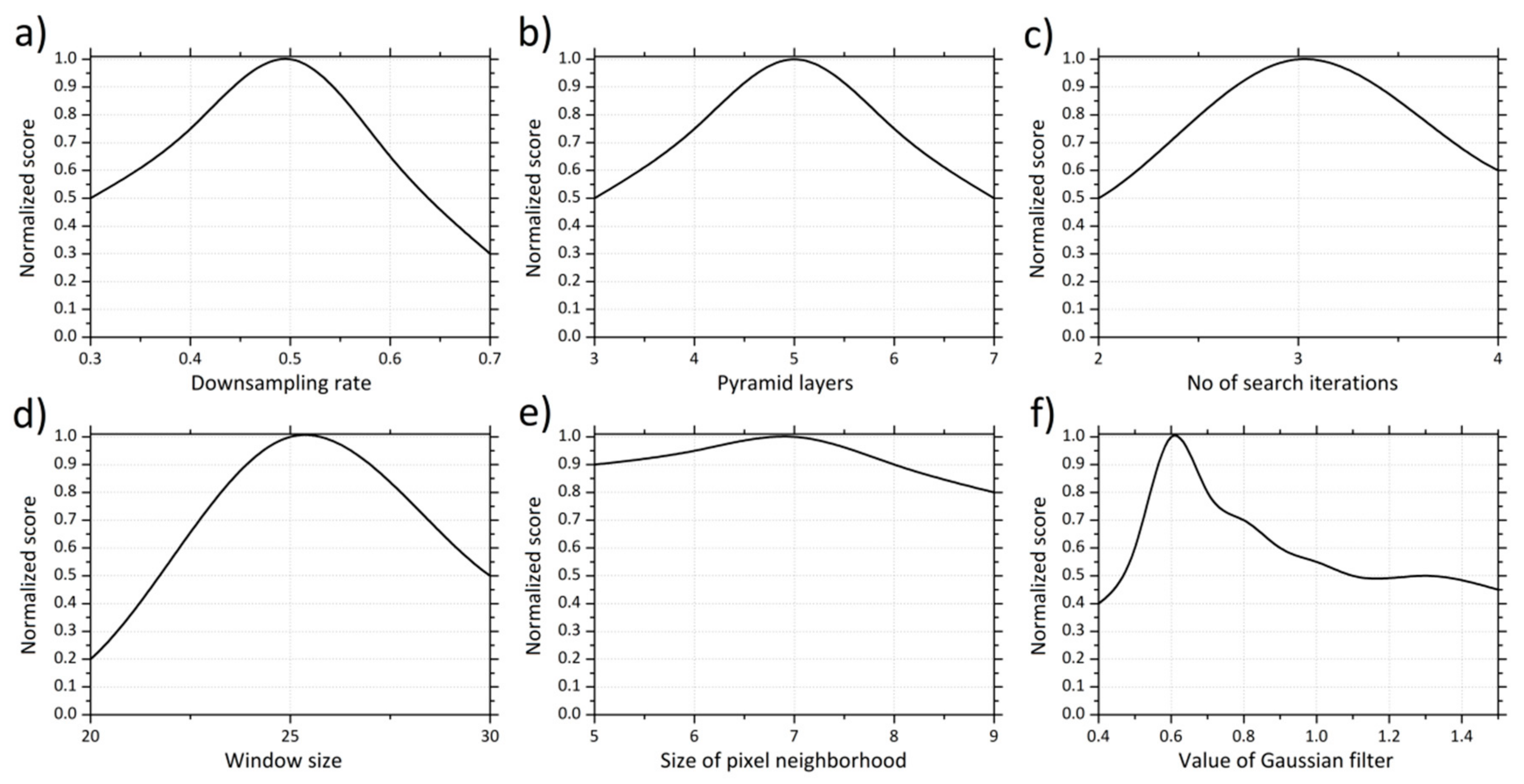
Figure 2 illustrates the FRB flowchart adapted to the specific parameters used in this study. Starting from the 1.45 million pixels images, the pyramid layers were set to 5 with a downsampling rate of 0.5 (i.e., each upper layer is twice smaller as the previous one) and a number of iterations equal to 3 in order to achieve the convergence of the pyramid layers transition to the final actual resolution image. Simultaneously, the window size was set to 25 since the optimum value should be large enough in order to have sufficient intensity variation and at the same time as small as to contain only pixels with about the same disparity. Finally, the size of the pixel neighborhood was set to 7 for smoother image surfaces and the standard deviation of the Gaussian filter to 0.6. The determination of the optimum parameterization for this study is shown in Figure 3, which highlights the contribution of the parameters to the optimum combination in terms of the normalized score, which is described as (X_max − X)/(X_max − X_min), where X represents each parameter value before the normalization, and the X_max and X_min are the maximum and minimum values of the range of the parameter, respectively.

2.2.3. TVL

The TVL algorithm [33] is an implementation of Zach et al. [39] optical flow estimation method. As stated before, in order to solve Equation (3), an additional constrain is need. This method is a modification of the method proposed by Horn and Schunck [41] (HS), and the proposed algorithm is based on the minimization of the following energy functional:

(6)

where $\mathsf{\rho }\left(\overrightarrow{\mathrm{u}}\right)$ term is the error that is introduced by a general image sequence, due to the assumption that governs Equation (3) (i.e., that image data are continuous in time) and λ is the parameter that weights between these two terms. The motivation of TVL penalizations is to handle discontinuities and/or occlusions where large errors are obtained with the original L2 regularization of the HS method. The proposed algorithm is a relaxed version of Equation (6), which is solved numerically by alternating minimization, using Chambolle’s algorithm [42] and point-wise thresholding. Similar to FRB, it is a two-frame method and also, in order to handle large displacements, the algorithm implements a pyramidal scheme to calculate the optical flow, starting from the coarsest level of the input images using the results as an input in the finer levels.

The implementation of the TVL algorithm was made using the OpenCV [40] functions. Perez et al. [33] give a detailed description of the 7 parameters needed as input, and on the OpenCV website, 5 additional technical inputs are given with their description. For the purposes of this study, the default values for all parameters were used. These input parameters are related to the precision and the running time of the numerical scheme, the pyramidal approach of the method, the a priori displacement field, the smooth filtering and an extra illumination.

2.3. Fast Radiative Transfer Model

For the FRTM, we used a novel model that is able to use operational and in real-time atmospheric inputs from earth observation (EO) data sources, like the COT from the MSG/SEVIRI applied in this study, and to produce massive DSSI outputs in high spatial, temporal and spectral resolutions of the order of 5 km, 15 min and 1 nm, respectively, as described in [36]. It uses a synergy of precalculated lookup tables (LUT) simulated by the libRadtran library of RTM [43], CMV algorithm as described in the previous Section 2.2 and high-performance computing (HPC) for parallel runs. Using a 32 core CPU supercomputer with 256 Gb RAM, the whole procedure (20 million simulations) runs for 1 min and 40 s, creating 12 high-resolution (1.5 million pixels) maps for the following 3 h. Figure 4 illustrates the data flow between the input used in this study to the FRTM and the DSSI output for 30 April 2020 at 12:00 UTC. A web service demonstration of the FRTM for the European and North African domains can be found online [44].

2.4. Statistical Tools

The results are evaluated in terms of mean bias and root mean square error (MBE and RMSE, respectively), defined in absolute terms as follows:

$$\mathrm{MBE}=\overline{\mathsf{\epsilon }}=\frac{1}{\mathrm{N}}{\displaystyle \sum }_{\mathrm{i}=1}^{\mathrm{N}}{\mathsf{\epsilon }}_{\mathrm{i}}$$

(7)

$$\mathrm{RMSE}=\sqrt{\frac{1}{\mathrm{N}}{{\displaystyle \sum }}_{\mathrm{i}=1}^{\mathrm{N}}{\mathsf{\epsilon }}_{\mathrm{i}}^2}$$

(8)

where ε_i = x_f − x₀ are the residuals calculated as the difference between the forecasted values (x_f) and the real observed values (x₀), and N is the total number of values. RMSE describes the overall spread of the error distribution, while MBE quantifies the bias and additionally detects overestimations (MBE > 0) or underestimations (MBE < 0). Finally, the mean absolute error (MAE), the correlation coefficient (r), as well as the standard deviation (σ) were used to represent the proportion of the variability between the forecasted and real observed values.

3. Results

3.1. Short-Term Forecasting Overview

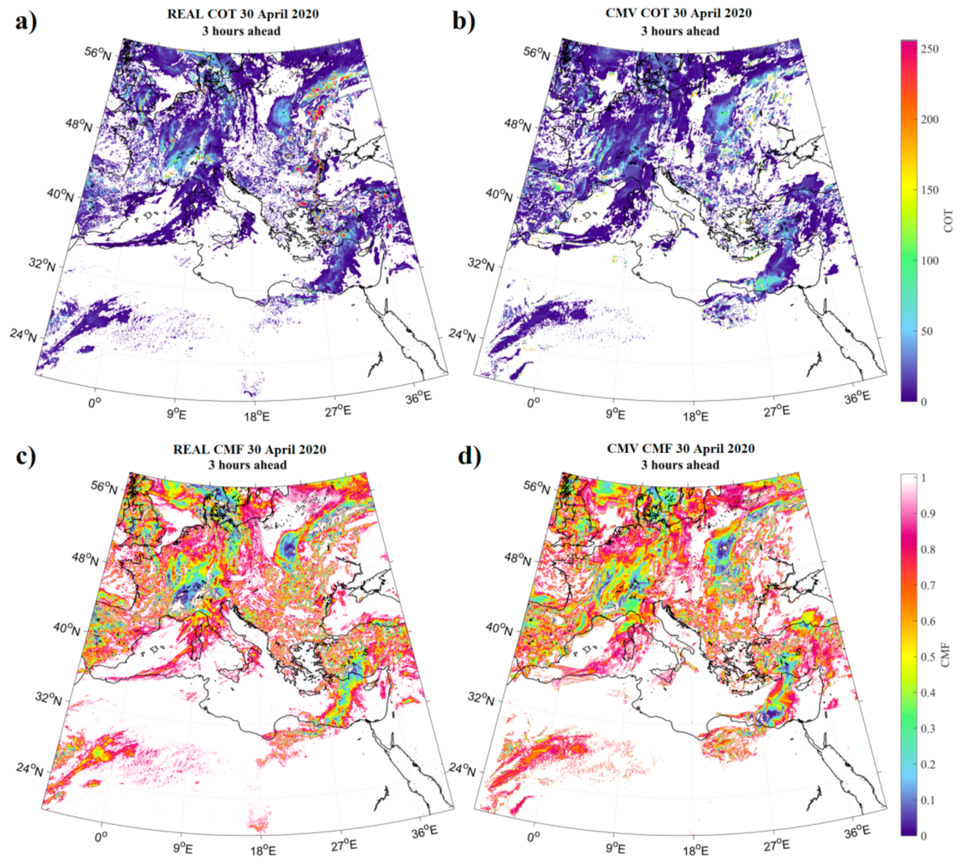
First of all, we developed two versions of the FRB motion flow technique. In the first one, we applied the motion flow to the COT parameter and in the second to the CMF. The idea behind this implementation was that the COT could potentially provide better results in terms of cloud formations monitoring. CMF corresponds to COT values from 0 to 3 since larger values, in reality, make the DSSI become almost zero. Hence, we made the hypothesis that if we use COT for the motion flow, maybe the additional information of COT values larger than 3 will follow better the cloud motion vectors. We also made some comparisons between FRB and the TVL motion flow approaches so as to identify the optimum conditions where both are able to provide much better results from the PRS method, where we keep clouds stationary, and all the other parameters (like SZA and aerosols) change dynamically. Before the application of the CMV method, the retrieval of CMF includes an extra step calculating it from COT by using the FRTM [36].

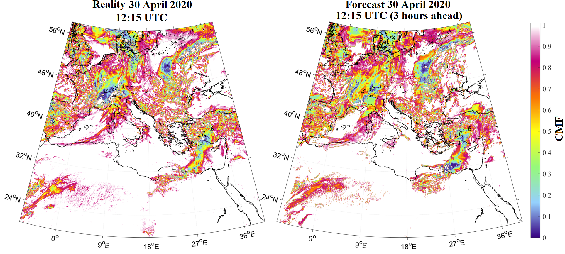
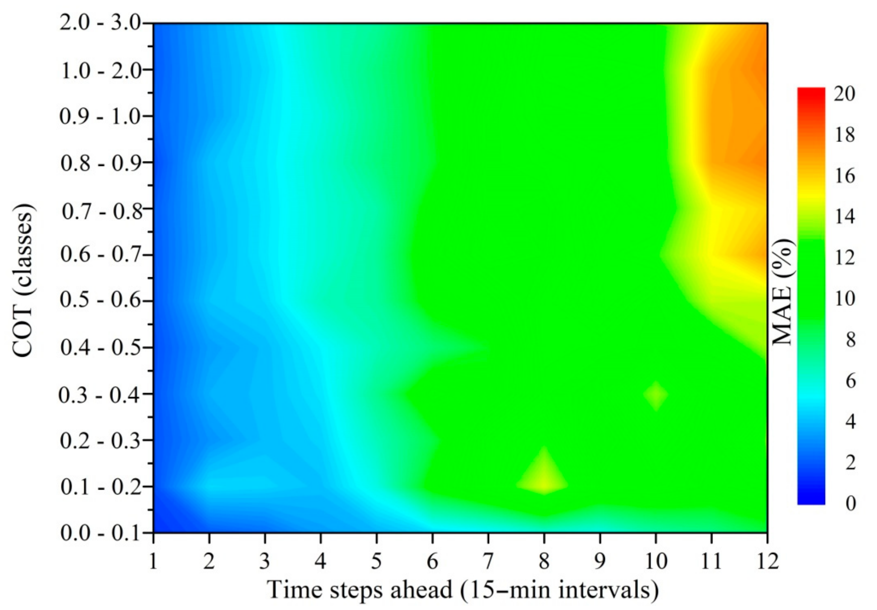
Figure 5 shows an example of the outputs. At the left maps (a) and (c) shows the real COT and CMF for 30 April 2020 at 12:15 UTC, and at the right maps (b) and (d) is the 3 h-ahead forecast based on the FRB method, starting from the training real time steps of 9:00 and 9:15 UTC. Figure 6 presents a contour plot of the MAE percentage of the FRB forecasted COT as a function of COT classes from 0 to 3 for the forecast horizon varying from 15 min to 3 h at an interval of 15 min. COT was classified using the real COT from the satellite for 30 April 2020 for the same coverage of Europe and North Africa.

It can be seen that the error increases significantly with the forecast horizon and is found to be higher for larger COT values. For most of the COT classes and forecast horizons, the error is found to be within 1%, while it is highest for the forecast horizon from 2 h 45 min to 3 h for the COT range of 0.6 to 3. The MAE percentage of COT is observed to be well within 5% up to 45 min forecast horizon for any COT classes. However, for forecast horizon from 45 min to 1 h 30 min, the MAE percentage of COT is within 5% for COT varying from 0 to 0.2, while it goes up to 12% for higher COT values. Beyond 1 h 30 min time horizon, the MAE percentage of COT varies from 6 to 12% for all COT classes, while it is found to go beyond 12% and to reach up to 20% for the forecast horizon from 2 h 45 min to 3 h for the COT range of 0.6 to 3.

3.2. FRB vs. TVL

Aiming to compare the two optical flow algorithms, we have made runs for both of them for the test days, using COT input. Figure 7 shows the RMSE and the MBE of CMF for the 3 days, starting from clear sky condition to cloudy condition. Both CMV techniques present better results from the PRS with much lower bias and forecast errors.

All statistics were calculated in terms of CMF to see the objective results, independently from solar elevation or other parameters like aerosols, etc., focusing only on the forecast cloud uncertainties and forecast horizon errors. A similar trend in error is seen from both FRB and TVL approaches for the 3-day analysis. However, FRB seems to produce slightly less error than the TVL method for all the days and all forecast horizons. The greatest difference is observed for 22 April 2020, during which FRB performs much better than the TVL approach for all forecast horizons, indicating the optimal performance of FRB under small-displacement conditions. This result is relatively different from the findings of [29,45] and must do with the optimization performed in this study to both CMV approaches. The TVL method has built-in smoothness terms that better handles cloud formation/dissipation, while FRB follows better multiple cloud layers with different directions and speeds. A similar evaluation approach was presented in [46], highlighting the usefulness of such comparisons (i.e., RMSE vs. MBE) for analyzing the forecast horizon statistics and the overall score. As a result, the overall accuracy of both CMV methods is strongly related to the specific characteristics of the cloud patterns, making a long-term (e.g., one full year of forecasts) validation necessary for more robust conclusions. For the rest of the study, we will focus on the FRB method, which appears to have equal or better results for the selected test days and also the easiest procedure for improving the model parameters [32]. It should be highlighted that this selection could not be generalized since further analysis is needed in terms of comparison against ground-based measurements.

3.3. COT vs. CMF

In order to investigate if COT or CMF is the most suitable parameter to apply optical flow techniques in order to calculate CMVs, both parameters were used, and the FRB method was applied for the three selected days.

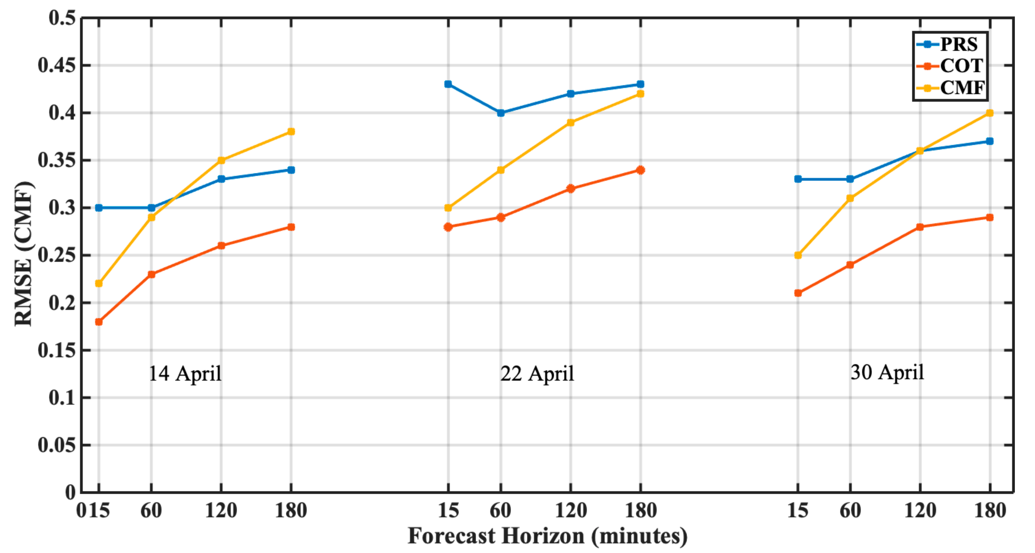
In Figure 8, we quantify the RMSE of CMF for pixels that changed from cloudy condition to clear sky and vice versa. The RMSE was calculated in terms of CMF for both cases of applying the FRB model to COT and CMF maps. The COT approach presents the lower error values for the 3 days, with the CMF approach to follow, and in some cases to be outperformed by the PRS at large forecast horizons, for example, at 2 and 3 h ahead of 14 April 2020 and at 3 h ahead of 30 April 2020. It is observed that the rate of increase in RMSE of CMF for PRS and COT is almost identical, while in the case of CMF, the rate is comparatively high. Surprisingly, both minimum and maximum RMSE values are observed in 15 min forecast as 0.18 for COT and 0.43 for PRS, respectively. The average RMSE of CMF is found to increase with forecast horizon as 0.28, 0.30, 0.34 and 0.36 for 15 min, 1 h, 2 h and 3 h forecasts, respectively.

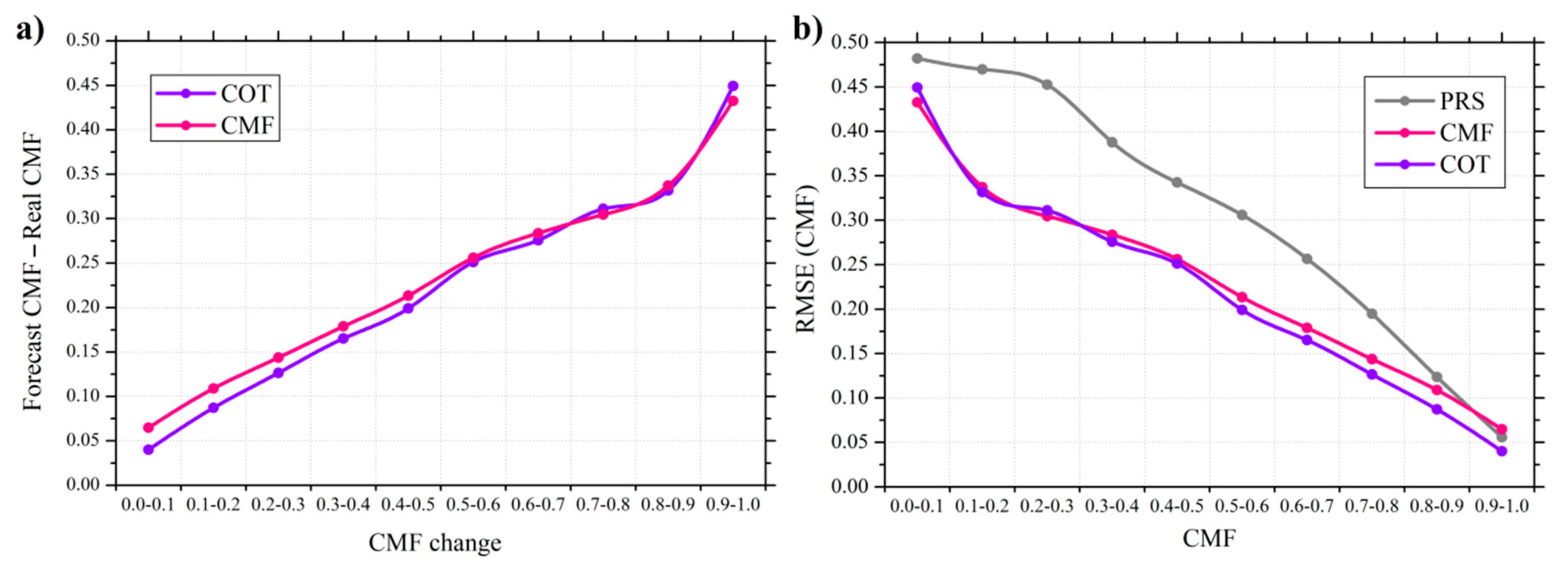
In Figure 9a, a quantification of the overall forecast variability for all CMF changes was performed. The horizontal axis shows the CMF change over two consecutive images, and the vertical axis represents the mean absolute difference between the forecast and the real CMF for both CMV approaches. Both COT and CMF techniques present similar behavior indicating the expected differences across the CMF potential changes.

The error between the forecasted and the real values of COT and CMF increases almost linearly with the increase in the change in CMF till 0.8, and the error is slightly more in the case of CMF than COT. However, a steep increase is seen beyond 0.8 CMF change. In Figure 9b, we show the RMSE for the CMF classes (classified by the actual CMF from satellite data), only for the cloud TRNs throughout the days and forecast horizons for both CMV approaches and the PRS method. The cloud TRNs mean the TRNs from cloudy conditions to clear sky and from clear sky to cloudy conditions of any CMF. This plot highlights the limited ability of the PRS to follow the CMF changes, especially at higher cloudy conditions with high COT values and low CMF values. The RMSE is seen to decrease in general with the increase in CMF. The declining RMSE curve for COT and CMF is observed to be almost identical and linear beyond 0.3 CMF, with the CMF RMSE being on a slightly higher side. However, the PRS declining curve is showing many deviations from the CMF and COT curves, with the deviation being maximum from 0.1 to 0.4 CMF range and decreases beyond 0.4 to zero at 0.9–1.0 CMF range. In general, forecasting COT provided better results; thus, this is the approach used for the rest of this study. In cases of changing cloudy conditions, CMV approaches outperformed the PRS and had comparable results.

3.4. CMV vs. PRS

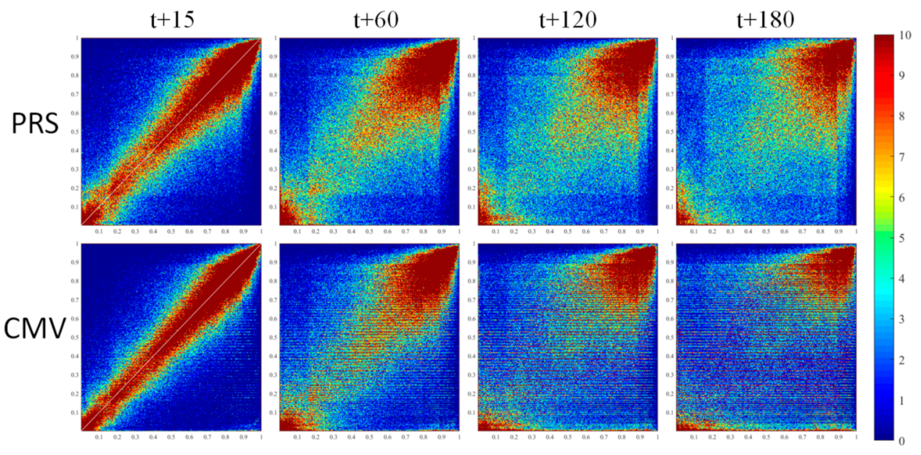
Figure 10 shows, for 30 April 2020, the density scatter plots for the PRS and FRB forecasted COT approaches, for 15 min, 1 h, 2 h and 3 h ahead, against real SEVIRI COT retrievals. A first quick result from this slide is that the PRS method, the PRS method where we follow the solar elevation and the only thing that stays persistent is the position of the clouds, has a larger scatter in comparison to the FRB approach. This is a result of the changing cloud conditions, which by definition, PRS cannot forecast.

As the forecast horizon increases from 15 min to 3 h, the coefficient of determination is seen to decrease, and the RMSE of COT is observed to increase. For 15 min forecast horizon, both the methods are performing quite well, with the correlation coefficient and RMSE of COT being 0.82 and 0.18 for the SPR method and 0.89 and 0.14 for the FRB method, respectively. However, as the forecast horizon increases from 15 min to 3 h, the coefficient of determination is seen to decrease from 0.82 to 0.5 for PRS and from 0.89 to 0.54 in the case of the FRB method. Moreover, the RMSE of COT increases from 0.18 to 0.31 for PRS and from 0.14 to 0.29 in the case of the FRB method. This indicates that the assumption of PRS that the cloud position remains unchanged is failing and leading to higher errors than the CMV method (FRB in this case) with an increased forecast horizon.

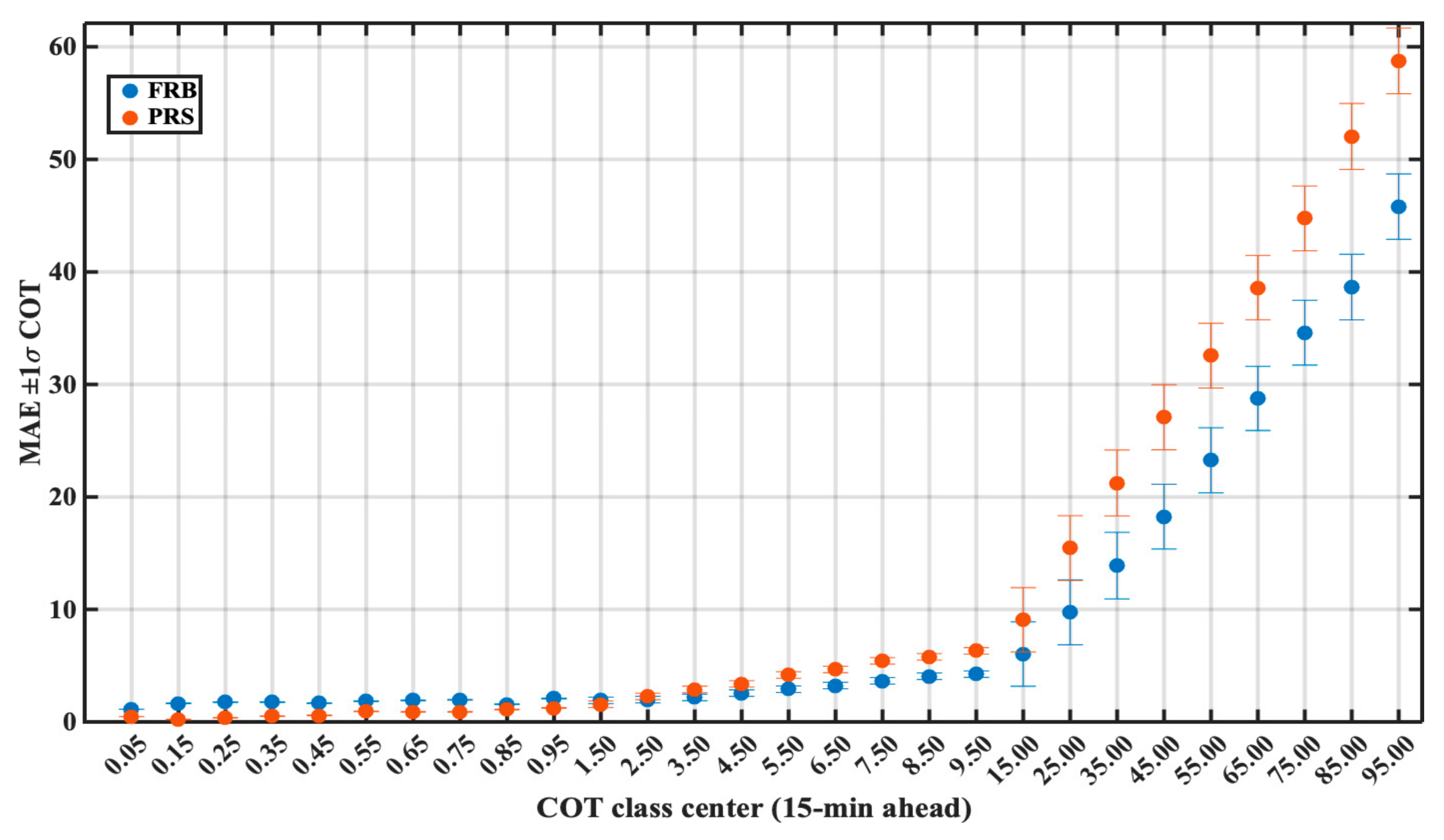
Figure 11 presents the MAE of FRB and PRS forecasted COT in the 15 min forecast time horizon for different real COT classes for the corresponding time step. The MAE of COT is found to be close to zero for real COT values ranging from 0 to 1 for both models. However, MAE of COT starts increasing beyond real COT value 1, but stays well within 8 below real COT value of 15 and increases sharply beyond that. The rate of increase of the MAE of COT is found to be higher in the case of PRS than that of FRB forecasts. CMV method is seen to perform better than the PRS for higher COT values.

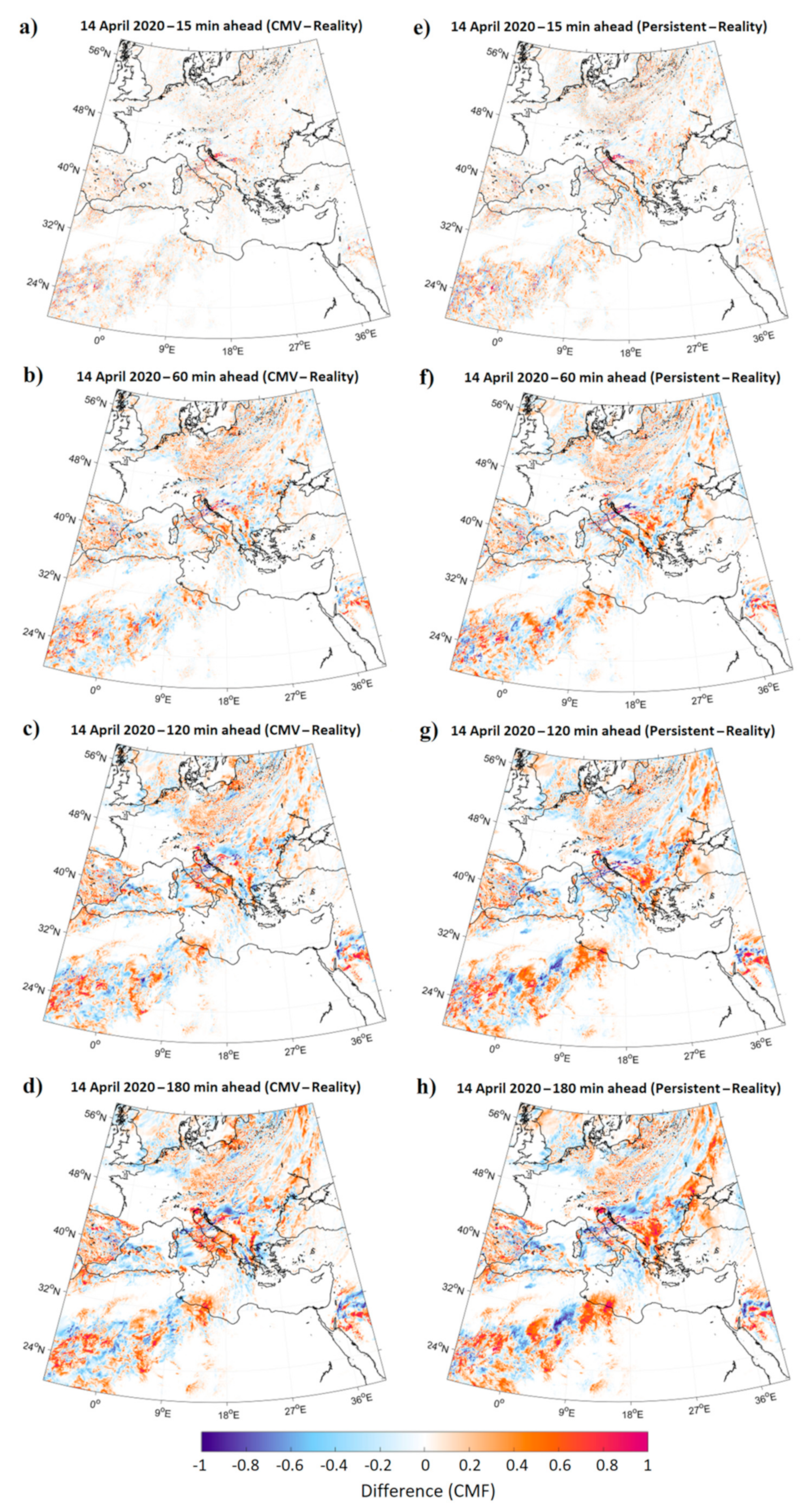
Figure 12 shows for 14 April 2020 the differences between FRB forecasted and real CMF for 15 min, 1, 2 and 3 h ahead at the left column and at the right column the same for the PRS. For both methods, the deviation from real CMF values is close to zero for 15 min forecasted time step and is increasing with the time horizon, as indicated with the increasing and more intense red and blue areas on the maps. A combination of underestimation and overestimation is seen for the forecast horizon varying from 1 to 3 h for both PRS and CMV methods.

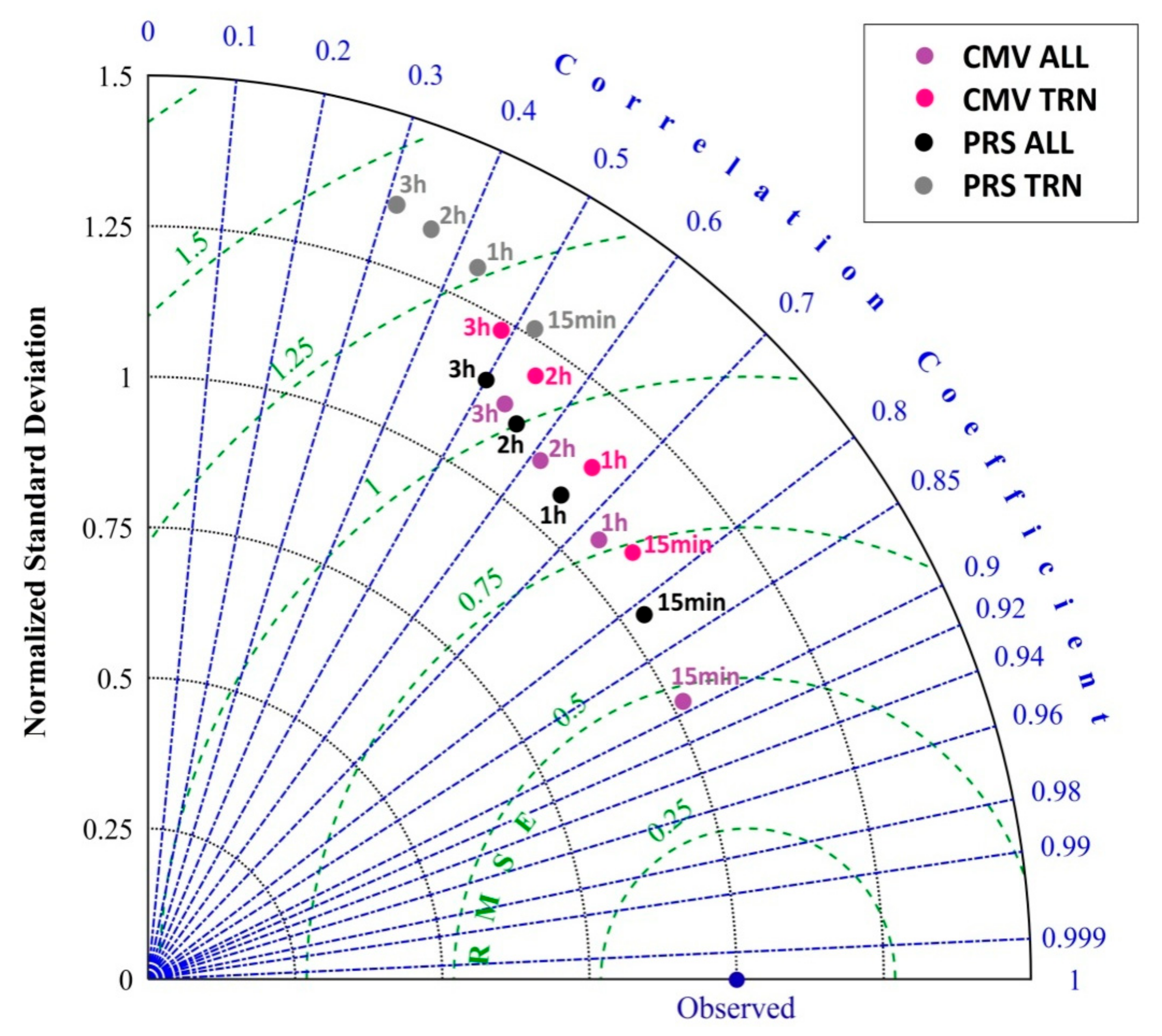
Figure 13 presents a Taylor diagram [47] with the overall CMF error for the PRS and the FRB COT forecasts as a function of the correlation coefficient, normalized RMSE and normalized standard deviation under all conditions and during TRN conditions. The use of this diagram was highlighted by numerous forecasting evaluation studies dealing with point-based comparisons as well as with image-based validation [48,49]. A note for this kind of analysis is that the PRS in some cases, like going from cloudy to clear sky conditions, presents better results than starting from clear sky to cloudy sky because returning to clear sky or CMF equals to one means that we go back to the optimum operating conditions for PRS, which are the clear sky conditions. Hence, taking into account that for the studied region, which has almost 1.5 million pixels, the majority is clear sky, around 700 to 800 thousand pixels, it is obvious that PRS is the prevailing situation that will have comparable performance to the CMV. Moreover, this is the main reason that we decided to focus as well on the sky conditions changes and the TRN between clear and cloudy sky.

Under all conditions, the CMV shows the best results/statistics with a correlation coefficient (r) close to 0.9 and the normalized standard deviation almost 1 for the 15 min-ahead time horizon. The r decreases to 0.54 for the 3 h-ahead time horizon, while the PRS under the same evaluation conditions presents similar statistics as the forecast horizon grows (i.e., r = 0.5 for 3 h ahead). The limited ability of the PRS method was revealed during the TRNs. Indicatively, the lowest r (~0.5) of the CMV TRN which is at the 3 h-ahead time horizon is almost the starting point of the PRS TRN at the 15 min ahead, highlighting the overall value of the CMV against the PRS.

Overall, the error from CMV and PRS increases significantly with the forecast horizon. It is also found to be greater for larger COT values. This is consistent with the density scatter plots, which show that PRS has a larger dispersion in comparison to the CMV approach, while the r decreases and the RMSE increases with the forecast horizon from 15 min to 3 h ahead. As the forecast horizon increases, the COT forecast accuracy decreases. The PRS method is based on the assumptions that clouds are stationary and all the other parameters, including the solar zenith angle and aerosol, change dynamically, which works fine for small forecast horizons but are producing higher errors at larger forecast horizon and especially during TRS conditions as is seen from the results. This is found to be consistent with the observation revealed from the comparison of the forecasts with reality. The quantification of RMSE for the clouds’ presence TRNs for the 3 days presents the COT approach as a lower error model followed by the CMF approach, and in some cases, to lose by the PRS approach at large forecast horizons. This claim is also supported by the observations seen from the quantification of the overall forecast variability, which showed that the COT and CMF techniques present similar behavior of a linear increase between the forecasted and the real values of COT and CMF with slightly more deviation in case of CMF than COT and the limited ability of the PRS to follow the CMF changes, especially, at higher cloudy conditions with high COT and low CMF values.

4. Conclusions

Solar forecasting up to 3 h requires cloud coverage at a bigger spatial scale with high temporal resolution. Hence, the extrapolation of future cloud locations is conventionally conducted using CMVs. This study aims at solar forecasting up to 3 h using satellite data with cloud forecasts at high spatial and temporal resolutions. This study presented two different CMV-based methods (FRB and TVL), each one using two different approaches; estimating optical flow by applying the brightness constancy assumption on COT and CMF. The tested methods were compared with a PRS method, trying to quantify the differential point of view of these techniques and the errors behaviors, as well as the conditions that the PRS approach cannot follow. The optical flow algorithms were implemented using satellite-derived COT maps provided by EUMETSAT SAF and CMF maps built up using the provided COT and FRTM with a high spatiotemporal resolution, wide spatial coverage covering Europe and North Africa, and capability for massive real-time simulations. The validation was conducted using the actual values of those parameters. In the first version of the FRB motion flow technique, motion flow was applied to the COT parameter and in the second to the CMF. A comparison between FRB and the TVL motion flow approaches was carried out to identify the optimum conditions where both are able to provide much better results from the PRS method, where we keep clouds stationary, and all the other parameters (like SZA and aerosols) change dynamically. A similar trend in error was observed from both FRB, and TVL approaches. However, FRB seemed to be a better approach than the TVL method in case of error statistics, especially under small-displacement conditions. In addition, the FRB is better under TRS conditions, while the PRS method can follow the CMVs only under continuously cloudless conditions.

The analysis has revealed that the error from the CMV and PRS model increases with COT and that the CMV methods are seen to outperform the PRS model for higher COT values. The correlation between the forecasted and the actual data were seen to deteriorate with the increasing forecast horizon (from 15 min to 3 h). A location and temporal-based comparison of FRB with PRS can determine in the future a hybrid approach on using the two methods with spatiotemporal based weights, exploiting the advantages of both methods. The comparison of the forecasts with the observed MSG/SEVIRI reference images also showed that the COT approach presents a lower error, followed by the CMF approach and the PRS, which cannot follow the forecast especially during sky condition TRNs. Unfortunately, none of these methods can properly deal with all of the many challenges that exist simultaneously in highly dynamic natural phenomena where the objects have no definitive features (e.g., cloud, water) or many similar features (e.g., orographic cloud streets). Brightness constancy is routinely violated in such cases, and if local features do exist they can move rapidly compared to their size. Moreover, this because statistically speaking, it is not so easy to trap the PRS scores.

As a next step, a massive forecast run for a whole year of COT data will be performed based on the CMV COT approach in order to compare with ground-based measurements across Europe and to make a model intercomparison with similar modeling approaches [29]. Particularly, after this study in which the CMV uncertainty was evaluated against the real MSG COT images and almost 60 million pixels in terms of CMF, an additional study followed by different comparison principles (i.e., earth observations vs. ground truth) is necessary in order to quantify the discrepancy between the simulated short-term forecasts and the ground measured irradiation, indicating the logic of the followed two-step evaluation approach [36]. Finally, the forthcoming Meteosat third-generation (MTG) satellites will increase the spatial resolution to almost 300 m, making the large-scale CMV approaches more accurate and, at the same time, even more complex and computationally expensive.