Full-Order Sliding Mode Observer Based on Synchronous Frequency Tracking Filter for High-Speed Interior PMSM Sensorless Drives

Abstract

In the research of the high-speed sensorless control strategy of an interior permanent-magnet synchronous motor (IPMSM), considering the harmonic influence of inverter nonlinearity on traditional sliding mode observer method, a full-order sliding mode observer (SMO) method based on synchronous frequency tracking filtering is proposed. This method avoids the phase delay defects caused by the use of filters in traditional second-order SMO. Then, the observed extended electromotive force (EMF) signal is filtered using a synchronous frequency tracking (SFT) function. It tracks the changing stator current and filters out harmonics that are not part of the tracking signal to achieve static tracking of the stator current. Then, the rotor speed can be estimated by a Luenberger-based observer. Experimental results verify the effectiveness and feasibility of the proposed method.

1. Introduction

Electric vehicle technology is a multi-disciplinary integrated technology of mechanics, power electronics, electrochemistry and control [1]. With the advantages of the stable installation structure of the permanent magnet, IPMSM has higher reliability [2]. Vector control has been widely adopted as the control strategy for IPMSM in electric vehicle applications. For the high-performance motor-driving applications, accurate detection of the rotor angle is the key to the frequency conversion control systems, especially when motors are used at high-speed applications [3]. Existing motor position detection methods can be classified into mechanical position sensor-based method and sensorless control method. The mechanical sensor method is to place a position transducer on the shaft of the rotor, like a mechanical encoder or a Hall sensor [4]. With the rapid development of electric vehicles, safety and reliability issues have increasingly become the focus of attention, and safety and reliability design in the process of vehicle design plays a pivotal role [5]. However, coupling structures are costly, unstable and complex due to the installation of mechanical sensors. Moreover, the mechanical sensor is affected by the circumstances such as high temperature or low temperature, thus affecting the performance of position-detecting in special environment [6,7]. Therefore, research on position sensorless control methods has received much attention in the past decades [8].

The sliding mode observer (SMO)-based control is one of the most conventional methods for the medium and high speed sensorless control [9,10]. SMO has the advantage of strong robustness to interference and insensitivity to the system parameter variations [11]. However, SMO uses discontinuous switch function, resulting in the chattering problem in the system. In addition, a low pass filter (LPF) is generally utilized to alleviate the chatting issue, which causes phase delay [12]. In [13], an adaptive structure for conventional, super-torsional and high-order sliding mode schemes is studied. The goal is to change the modulation gains associated with these schemes so that they are as small as possible to mitigate buffeting effects, but large enough to ensure that they remain sliding in the face of bounded and derivative bounded uncertainties [14]. In [15], aiming at the control problem of electropneumatic actuators, a new super-torsional adaptive sliding mode control law is proposed. The main point of [15] is to consider the uncertainty, and the boundary of the disturbance is unknown [16]. These methods improved the chattering problem of the traditional synovial membrane. In [17], with the purpose of avoiding the phase retardance of the LPF in sliding mode control, a new technique based on fractional phase-locked loop (PLL) is proposed, in which the fractional PLL provides additional degrees of freedom by the selection of proper fractional order. However, this method does not apply to the wide speed range of PMSM. Reference [18] proposes a quadrature PLL comprising two synchronous frequency extraction filters, which estimates the rotor position angle by calculating the fundamental harmonic component of the estimated back-EMF. Because it retains the traditional SMO link, the harmonic signals are not completely eliminated. The rotor position angle is calculated from the inverse tangent of the estimated back-EMF, which causes the estimation error of the back-EMF and an inaccurate estimation of the rotor position and speed.

Moreover, due to electromagnetic and mechanical errors, temperature changes, and nonlinearities of the driving inverter, there are many harmonics in estimating back-electromotive force (back-EMF) [9,10,11,12]. These harmonics affect the accuracy of the rotor position and speed estimation. Based on the model-based sensorless control method, S. Jung et al. [19] proposed an accurate mathematical model considering spatial harmonics of inductance. However, this method requires off-line debugging, which increases the complexity of the system. In [20], a new sensorless speed control method is proposed, which combines SMO and a model reference adaptive system (MRAS). The combined method can simultaneously ensure the estimation convergence of both velocity and position. With the aim of eliminating the torque fluctuation and mitigating the impact of the back EMF’s harmonics estimated by the SMO, a variable frequency stator current-tracking method according to the output regulation is introduced, which accurately estimates the back EMF. The enhanced control method has higher precision in rotor position and speed estimation, and can maintain high-accuracy estimation of the rotor even at the scenario of low-speed cases.

In addition, other methods have gradually attracted attention in recent years, including the extended Kalman filter (EKF) [21,22], recursive least squares (RLS) [23], artificial neural network (ANN) [24], full-order observer [25] and reduced-order observer [26]. In [21], satisfying rotor flux estimation results are obtained through the EKF technique. However, this suffers from the demerits of complex algorithm structures, parameter adaptation difficulties and initialization problems, and inattentiveness to disturbance. The RLS method for electrical parameter estimation proposed in [23] provides a fast converging rate. However, because of the large number of differential equations incorporated, the performance of the controller is reduced, and the system response is slow. In [25], a full-order observer is used to estimate the stator current. Although its robustness is good, the accurateness of the full-order observer relies on other motion factors. In addition, the sign of gain matrix for the observer is pretty complex. In [26], a reduced-order observer with respect to the rotor flux is proposed, while the mechanical parameters are eliminated. However, the current value obtained from the sensor is impacted by the noise and interference. Thus, the reduced-order rotor flux observer brings distortion of the estimated parameters. Although the location estimation methods proposed by the predecessors have unique characteristics and reasonable performance, these methods still have certain limitations or deficiencies in theory.

This paper proposes using a full-order SMO method based on synchronous frequency tracking filtering to track the fundamental wave of s the estimated back-EMF. Therefore, a proposed speed-estimation method merging the full-order SMO, SFT Heterodyne and LBO establish this tracking strategy to support IPMSM motors in wide speed applications. Therefore, the proposed method is of great significance to industry applications, like the electric vehicle (EV) system, the air-conditioning system, the elevator and assembly line.

2. The Method of Position Estimation Based on the Traditional Second-Order SMO

2.1. Extened EMF Model of IPMSM

Unlike the surface PMSM, the d and q axis inductance of IPMSM is not equal. Therefore, under the d-q axis, the voltage equation for IPMSM is

$$\left[\begin{array}{l}{u}_d\\ u_q\end{array}\right]=\left[\begin{array}{cc}{R}_s+p{L}_d& -{\omega }_e{L}_q\\ {\omega }_e{L}_d& R_s+p{L}_q\end{array}\right]\left[\begin{array}{c}{i}_d\\ i_q\end{array}\right]+\left[\begin{array}{c}0\\ {\omega }_e{\psi }_f\end{array}\right]$$

(1)

where p is the derivative operator, u_d and u_q are the d–q axis stator voltage components, i_d and i_q are the d–q axis stator current components, L_d and L_q are the d–q axis inductance, R_s is the stator-winding resistance, ω_e is the rotor mechanical speed and ψ_f is the flux linkage of the rotor magnets.

By changing the Equation (1) as follows, the position information of the IPMSM rotor can be obtained to make it symmetrical

$$\left[\begin{array}{l}{u}_d\\ u_q\end{array}\right]=\left[\begin{array}{cc}{R}_s+p{L}_d& -{\omega }_e{L}_q\\ {\omega }_e{L}_q& R_s+p{L}_d\end{array}\right]\left[\begin{array}{c}{i}_d\\ i_q\end{array}\right]+\left[\begin{array}{c}0\\ E_{ex}\end{array}\right]$$

(2)

where E_ex = (L_d − L_q)(ω_ei_d − pω_ei_q) + ω_eψ_f, and E_ex is named as extended EMF. It consists of a traditional back electromotive force ω_e, ψ_f and the (L_d − L_q)(ω_ei_d − pω_ei_q) produced by the salient pole characteristics of IPMSM. Figure 1 shows the physical model of the IPMSM.

2.2. Traditional Second-Order SMO of IPMSM

The traditional second-order SMO constructs the PMSM position observer using the mathematical models of the α-βaxis motor [27,28,29,30,31,32]. This is due to the fact that the mathematic model of the rotating coordinate system obtained from the Park transformation needs the position information θ_e of the rotor. The control system adopts the qd0 model [29]. Figure 2 shows the schematic diagram of a traditional second-order SMO [31].

Therefore, in the α-β axis, Equation (2) becomes

$$\left[\begin{array}{l}{u}_{\alpha }\\ u_{\beta }\end{array}\right]=\left[\begin{array}{cc}{R}_s+p{L}_d& {\omega }_e(L_d-L_q)\\ -{\omega }_e(L_d-L_q)& R_s+p{L}_d\end{array}\right]\left[\begin{array}{c}{i}_{\alpha }\\ i_{\beta }\end{array}\right]+\left[\begin{array}{c}{e}_{\alpha }\\ e_{\beta }\end{array}\right]$$

(3)

where

$$e_{\alpha }=-E_{ex}\sin {\theta }_e,e_{\beta }=E_{ex}\cos {\theta }_e$$

(4)

and they are the extended EMF components on the α-β axis. As found in Equation (3), the rotor position information only appears in the extended EMF. Thus, the Equation (3) is written as follows

$$\frac{d}{dt}\left[\begin{array}{l}{i}_{\alpha }\\ i_{\beta }\end{array}\right]=\frac{1}{L_d}\left[\begin{array}{cc}-R_s& -{\omega }_e(L_d-L_q)\\ {\omega }_e(L_d-L_q)& -R_s\end{array}\right]\left[\begin{array}{c}{i}_{\alpha }\\ i_{\beta }\end{array}\right]+\frac{1}{L_d}\left[\begin{array}{c}{u}_{\alpha }-e_{\alpha }\\ u_{\beta }-e_{\beta }\end{array}\right]$$

(5)

Selecting the sliding surface s(x) = 0 on the stator current, thus

$$s(x)=\left[\begin{array}{c}{\tilde{i}}_{\alpha }\\ {\tilde{i}}_{\beta }\end{array}\right]=\left[\begin{array}{c}{\widehat{i}}_{\alpha }-i_{\alpha }\\ {\widehat{i}}_{\beta }-i_{\beta }\end{array}\right]=0$$

(6)

where, ${\widehat{i}}_{\alpha }$ and ${\widehat{i}}_{\beta }$ are the current values observed under the α-β axis, ${\tilde{i}}_{\alpha }$ and ${\tilde{i}}_{\beta }$ are the difference in value between the estimated and the actual values, respectively.

Using i_α and i_β as state variables, and the SMO equation is derived as follows from Equation (5)

$$\frac{d}{dt}\left[\begin{array}{l}{\widehat{i}}_{\alpha }\\ {\widehat{i}}_{\beta }\end{array}\right]=\frac{1}{L_d}\left[\begin{array}{cc}-R_s& -{\widehat{\omega }}_e(L_d-L_q)\\ {\widehat{\omega }}_e(L_d-L_q)& -R_s\end{array}\right]\left[\begin{array}{c}{\widehat{i}}_{\alpha }\\ {\widehat{i}}_{\beta }\end{array}\right]+\frac{1}{L_d}\left[\begin{array}{c}{u}_{\alpha }-z_{\alpha }\\ u_{\beta }-z_{\beta }\end{array}\right]$$

(7)

where, ${\widehat{\omega }}_e$ is the estimated rotor speed, $z_{\alpha }$ and $z_{\beta }$ are the control components for the α–β axis, and where k is the sliding mode gain, and it is a normal number which is large enough to ensure that the observer is stable, and sign represents the sign function.

$$\left[\begin{array}{l}{z}_{\alpha }\\ z_{\beta }\end{array}\right]=k\left[\begin{array}{c}sign({\widehat{i}}_{\alpha }-i_{\alpha })\\ sign({\widehat{i}}_{\beta }-i_{\beta })\end{array}\right]$$

(8)

The dynamic error equation can be obtained from Equations (5) and (7),

$$\begin{array}{l}\frac{d{\tilde{i}}_{\alpha }}{dt}=\frac{-R_s}{L_d}{\tilde{i}}_{\alpha }-\frac{(L_d-L_q)}{L_d}({\widehat{\omega }}_e{\widehat{i}}_{\beta }-{\omega }_e{i}_{\beta })-\frac{k}{L_d}sign({\tilde{i}}_{\alpha })+\frac{e_{\alpha }}{L_d}\\ \frac{d{\tilde{i}}_{\beta }}{dt}=\frac{-R_s}{L_d}{\tilde{i}}_{\beta }+\frac{(L_d-L_q)}{L_d}({\widehat{\omega }}_e{\widehat{i}}_{\alpha }-{\omega }_e{i}_{\alpha })-\frac{k}{L_d}sign({\tilde{i}}_{\beta })+\frac{e_{\beta }}{L_d}\end{array}$$

(9)

When the system enters the sliding surface, the observer speed ${\widehat{\omega }}_e$ will converge to the real value, ${\omega }_e$, and ${\widehat{\omega }}_e={\omega }_e$. At this time, Equation (9) can be simplified into Equation (10)

$$\begin{array}{l}\frac{d{\tilde{i}}_{\alpha }}{dt}=\frac{-R_s}{L_d}{\tilde{i}}_{\alpha }-\frac{(L_d-L_q)}{L_d}{\widehat{\omega }}_e{\tilde{i}}_{\beta }-\frac{k}{L_d}sign({\tilde{i}}_{\alpha })+\frac{e_{\alpha }}{L_d}\\ \frac{d{\tilde{i}}_{\beta }}{dt}=\frac{-R_s}{L_d}{\tilde{i}}_{\beta }+\frac{(L_d-L_q)}{L_d}{\widehat{\omega }}_e{\tilde{i}}_{\alpha }-\frac{k}{L_d}sign({\tilde{i}}_{\beta })+\frac{e_{\beta }}{L_d}\end{array}$$

(10)

When the system converges, s(x) = ds(x)/dt = 0, the current error ${\tilde{i}}_{\alpha }$ and ${\tilde{i}}_{\beta }$ approaches 0. The system operates steadily on the sliding surface, and the calculated extended back-EMF is expressed in the following

$$\left[\begin{array}{c}{\widehat{e}}_{\alpha }\\ {\widehat{e}}_{\beta }\end{array}\right]=k\left[\begin{array}{c}sign({\tilde{i}}_{\alpha })\\ sign({\tilde{i}}_{\beta })\end{array}\right]=\left[\begin{array}{c}-E_{ex}\sin {\theta }_e\\ E_{ex}\cos {\theta }_e\end{array}\right]$$

(11)

where ${\widehat{e}}_{\alpha }$ and ${\widehat{e}}_{\beta }$ are both the back-EMF obtained by a LPF from the sign function, and the rotor position angle passes can be obtained as

$${\widehat{\theta }}_e=-{\tan }^{-1}\left({\widehat{e}}_{\alpha }/{\widehat{e}}_{\beta }\right)$$

(12)

Normally, the rotor position signal of the IPMSM can be obtained by the inverse tangent function of ${\widehat{e}}_{\alpha }$ and ${\widehat{e}}_{\beta }$. However, the inverse tangent function will lead to large rotor position error especially when the back-EMF crosses zero. Furthermore, an estimate of the rotor speed is calculated by differentiation of the rotor angle, which amplifies the noise. Using LPF also causes phase delay errors. Traditional second-order SMO reduces the accuracy of the estimated speed, especially in the case of motor runs at low speeds.

Figure 3 shows a sensorless control method for an IPMSM employing the traditional second-order SMO. The accuracy of the method is verified by simulation. the IPMSM parameters for the test were listed in

Table 1. Parameters of the tested IPMSM.

Symbol	Quantity	Value
Vdc	Rated Voltage	220 V
I	Rated Current	14.7 A
n	Rated Speed	2500 r/min
S	Rated Power	2500 W
Rs	Resistance	0.7 Ω
Ld	d-axis Inductance	3.2 mH
Lq	q-axis Inductance	4.0 mH
p	Magnetic Pole Pairs	4

. The sensorless algorithm developed was simulated by MATLAB/Simulink. Simulation continuous operation t = 2 s, load torque Te = 0.5 Nm. The steady-state performance of the system at 1000 rpm was simulated.

The actual speed n and the estimated speed $\widehat{n}$ are compared in Figure 3a. It can be seen that the pulsation of the estimated speed is large, which is mainly due to many uncertainties such as inverter nonlinearity, electromagnetic and mechanical tolerances. This causes the estimated back-EMF to have more harmonic content. The speed error is about ±40 r/min. Figure 3b,c gives the actual position of the rotor θ_e and the estimated position ${\widehat{\theta }}_e$. As demonstrated by the enlarged waveform, the estimated rotor position is unstable and there is an obvious chattering phenomenon. Figure 3d illustrates the rotor position error waveform. The position error is large when the motor starts running, and then the error oscillates around 2.5°. Figure 3e shows the extended back-EMF component of the rotor position information observed by the conventional second-order SMO. As presented in this figure, the observed back-EMF component does contain a large number of harmonics. Figure 3f shows the harmonic spectrum obtained by Fast Fourier Transform (FFT), where the fundamental frequency is 66.67 Hz. Through the FFT analysis, the observed back-EMF mainly contains 3rd, 5th and 7th harmonics, which coincide preciously with the theoretical prediction. These harmonics and noise greatly reduce the accuracy of rotor position estimation. Therefore, with the traditional SMO method, the estimated speed error is large, and the accuracy of position observation is not high.

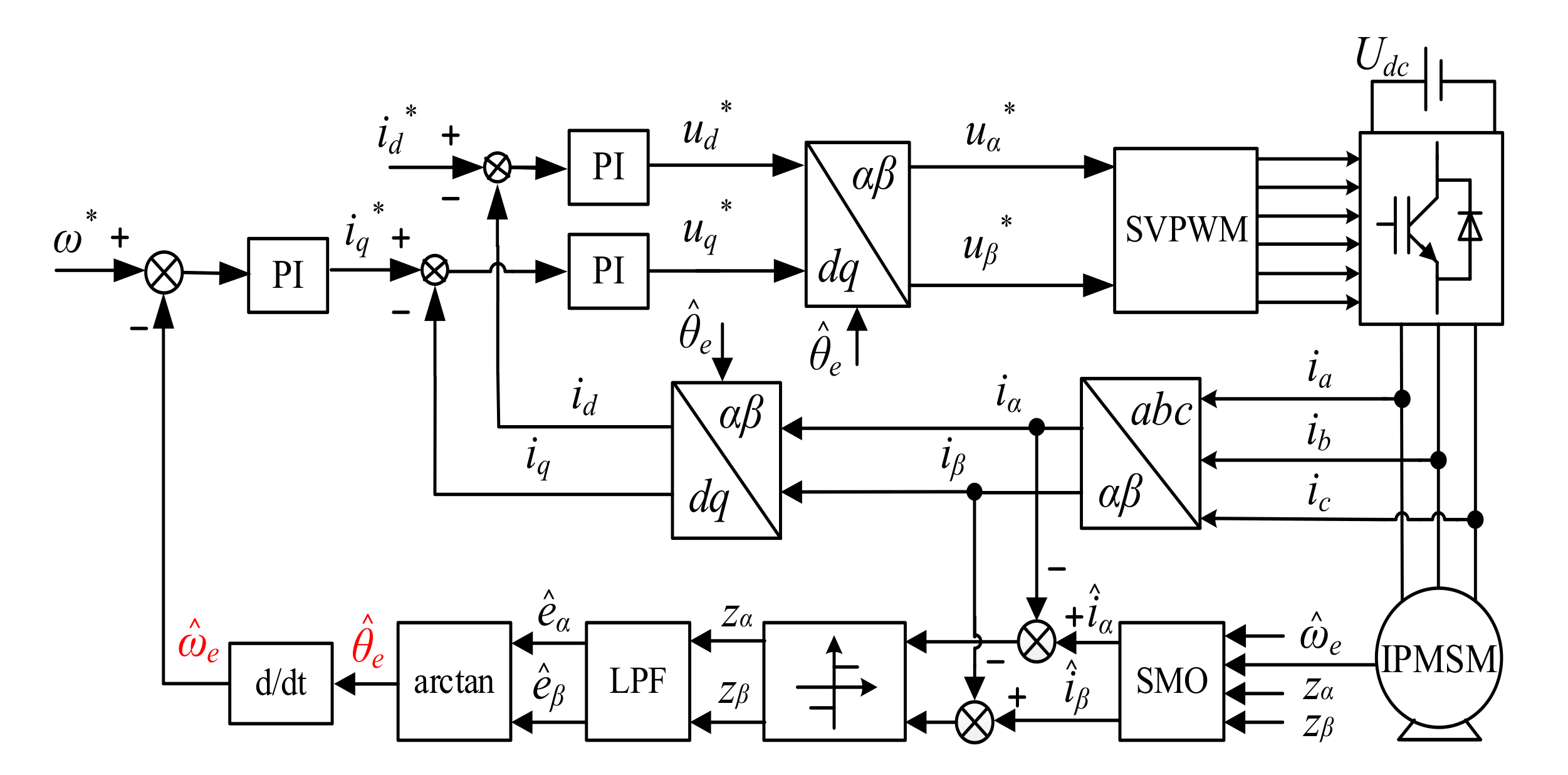
3. Proposed Rotor-Speed Sensorless-Control Method of Full-Order SMO Based on SFT Filter and Luenberger Observer

3.1. Full-Order SMO Method

For IPMSM, rewrite the current equation under the α-β axis

$$\frac{d}{dt}{\mathit{i}}_s={\mathit{A}\mathit{i}}_s+\mathit{B}\mathit{u}+\mathit{C}\mathit{e}$$

(13)

where

$$\begin{gathered} {\mathit{i}}_s={\left[\begin{array}{cc}{i}_{\alpha }& i_{\beta }\end{array}\right]}^T,\mathit{e}={\left[\begin{array}{cc}{e}_{\alpha }& e_{\beta }\end{array}\right]}^T,\mathit{u}={\left[\begin{array}{cc}{u}_{\alpha }& u_{\beta }\end{array}\right]}^T;\mathit{A}=-R_s/L_d\cdot \mathit{I}+{\omega }_e(L_d-L_q)/L_d\cdot \mathit{J}; \\ \mathit{B}=1/L_d\cdot \mathit{I},\mathit{C}=-1/L_d\cdot \mathit{I};\mathit{I}=\left[\begin{array}{cc}1& 0\\ 0& 1\end{array}\right],\mathit{J}=\left[\begin{array}{cc}0& -1\\ 1& 0\end{array}\right]. \end{gathered}$$

In the control system, since the speed variation rate is considerably smaller than the stator current variation rate, e_α and e_β, and their rate of change is written as

$$\frac{d}{dt}\left[\begin{array}{c}{e}_{\alpha }\\ e_{\beta }\end{array}\right]={\omega }_e\left[\begin{array}{c}-e_{\beta }\\ e_{\alpha }\end{array}\right]$$

(14)

A full-order SMO can be created by using Equation (14). Its state equation is

$$\frac{d}{dt}{\hat{\mathit{i}}}_s={\hat{\mathit{A}}\hat{\mathit{i}}}_s+\mathit{B}\mathit{u}+\mathit{C}\left(\hat{\mathit{e}}+\mathit{z}\right)$$

(15)

$$\frac{d}{dt}\hat{\mathit{e}}={\widehat{\omega }}_e\left[\begin{array}{c}-{\widehat{e}}_{\beta }\\ {\widehat{e}}_{\alpha }\end{array}\right]+\frac{1}{L_d}\mathit{D}\mathit{z}$$

(16)

where

$$\begin{gathered} {\hat{\mathit{i}}}_s={\left[\begin{array}{cc}{\widehat{i}}_{\alpha }& {\widehat{i}}_{\beta }\end{array}\right]}^T,\hat{\mathit{e}}={\left[\begin{array}{cc}{\widehat{e}}_{\alpha }& {\widehat{e}}_{\beta }\end{array}\right]}^T,\mathit{z}=\left[\begin{array}{l}{z}_{\alpha }\\ z_{\beta }\end{array}\right]=K\left[\begin{array}{c}sign({\widehat{i}}_{\alpha }-i_{\alpha })\\ sign({\widehat{i}}_{\beta }-i_{\beta })\end{array}\right], \\ \hat{\mathit{A}}=-R_s/L_d\cdot \mathit{I}+{\widehat{\omega }}_e(L_d-L_q)/L_d\cdot \mathit{J},\mathit{D}=\left[\begin{array}{cc}l& 0\\ 0& l\end{array}\right] \end{gathered}$$

where K and l are the stable SMO gain derived by Lyapunov function theorem. The state variables at this time is the E_ex component and the stator current.

According to Equations (14) and (16), the dynamic error equation of E_ex component is:

$$\frac{d}{dt}\left[\begin{array}{c}{\tilde{e}}_{\alpha }\\ {\tilde{e}}_{\beta }\end{array}\right]={\widehat{\omega }}_e\left[\begin{array}{c}-{\tilde{e}}_b\\ {\tilde{e}}_{\alpha }\end{array}\right]+\frac{1}{L_d}l\left[\begin{array}{c}sign({\tilde{i}}_{\alpha })\\ sign({\tilde{i}}_{\beta })\end{array}\right]$$

(17)

where ${\tilde{e}}_{\alpha }$ and ${\tilde{e}}_{\beta }$ represent the dynamic error of the estimated extended back-EMF component and the actual extended back-EMF component.

When the system enters the sliding surface, the estimated back-EMF can still be obtained by referring to the analysis process of the second-order SMO.

$$\left[\begin{array}{c}{\tilde{e}}_{\alpha }\\ {\tilde{e}}_{\beta }\end{array}\right]=K\left[\begin{array}{c}sign({\tilde{i}}_{\alpha })\\ sign({\tilde{i}}_{\beta })\end{array}\right]=\left[\begin{array}{c}-E_{ex}\sin {\theta }_e\\ E_{ex}\cos {\theta }_e\end{array}\right]$$

(18)

Substituting (18) into (17)

$$\frac{d}{dt}\left[\begin{array}{c}{\tilde{e}}_{\alpha }\\ {\tilde{e}}_{\beta }\end{array}\right]={\widehat{\omega }}_e\left[\begin{array}{c}-{\tilde{e}}_{\beta }\\ {\tilde{e}}_{\alpha }\end{array}\right]+\frac{1}{L_d}\frac{l}{K}\left[\begin{array}{c}{\tilde{e}}_{\alpha }\\ {\tilde{e}}_{\beta }\end{array}\right]$$

(19)

The above equation shows that the dynamic equation of the full-order SMO includes two links of filtering and correction, so that the LPF is not needed here. Thus, the phase delay defect generated by the LPF in the conventional second-order SMO method is avoided. The accuracy of position estimation is improved. Then, the obtained back-EMF is passed through the position observer to obtain the rotor position signal.

However, due to the influence of electromagnetic error, mechanical error and flux harmonic, the rotor position estimation error is still very large. These errors will affect the stability of the system and increase the loss of the system. In order to eliminate the influence, researchers have adopted corresponding methods in motor design, such as choosing permanent magnets with the same performance and permanent magnet materials with good temperature stability. However, the harmonic components in the estimated extended back-EMF are difficult to eliminate. There are a large number of 5th and 7th harmonic components in the estimated extended back-EMF due to the nonlinearity of the inverter [27,28], and this problem has always existed in power electronics applications. Therefore, eliminating harmonic components in the estimated back EMF due to inverter nonlinearity is the key to the SMO method.

3.2. Construction of Synchronous Frequency Tracking Filter

The harmonic estimation and error of the back-EMF will lead to the inaccuracy of rotor speed estimation. This will affect the accuracy and stability of velocity identification. To filter out the harmonics of the estimated back-EMF signal, a synchronous frequency tracking (SFT) filter is proposed. PR controller is used in SFT because PR controller can accurately track ac signals at a specified frequency [29]. The fundamental wave of the estimated back-EMF can be extracted from the original signal through the SFT filter. Meanwhile, the harmonic components in the back-EMF are reduced by the SFT filter. Therefore, this filter can be used to obtain the signal of the desired frequency and eliminate the harmonic signals of other frequencies, thereby achieving the purpose of tracking and filtering.

The influence of harmonic components on SMO can be overcome by using the proposed SFT. Figure 4 shows the block diagram of the SFT filter. The transfer function of SFT can be expressed as

$$\frac{Y(s)}{U(s)}=\frac{2K_r{\omega }_{c}s}{s^2+2{\omega }_{c}s+{(2\pi \widehat{f})}^2}$$

(20)

where $\widehat{f}$ is the stator current frequency obtained from the observed rotor speed ${\widehat{\omega }}_e$, $\widehat{f}={\widehat{\omega }}_e/2\pi$, K_r is the resonance gain, and ω_c is the cut-off frequency. U(s) is the input signal of the SFT filter, and it is the extended back-EMF component observed by the full-order SMO under the α-β axis. Y(s) is the output signal of the SFT filter. It contains rotor position information and then enters into the position observer, as shown in Figure 4. The obtained observation speed will be sent back to the $\widehat{f}$, which is the stator current frequency of the SFT filter to obtain the target of tracking filtering. During the actual operation of the motor, the frequency of the stator current changes with the variation in the speed. The SFT filter can track the varying frequency well.

In the IPMSM drive system, the stator current and the electromagnetic field of the α-β axis have the same frequency and the value is proportional to the estimated rotor speed [29,30]. Therefore, the resonant frequency of the SFT function is not a constant quantity, but a real-time variable speed feedback. Furthermore, static tracking of the stator current can be achieved with SFT.

The stability performance of the SFT is analyzed below. Figure 5a shows the pole-zero plot and root locus of the SFT function as ${\widehat{\omega }}_e$ increases. It can be seen that the SFT does not have poles and zeros with a positive real part. SFT is stable over the entire speed range. The real part of the pole is small (=−0.5).

Figure 5b shows the Bode plot of the SFT function when ω_c increases, at this time ${\widehat{\omega }}_e$ = 50 rad/s. In this figure, the three lines correspond to ω_c = 0.1 rad/s, ω_c = 1 rad/s and ω_c = 10 rad/s from the inside to the outside. All three lines are centered around ${\widehat{\omega }}_e$, meaning that the SFT function can accurately track the phase and amplitude at the same time. As the cut-off frequency of the SFT function ω_c is reduced, the signal extraction capability of the SFT function is enhanced.

However, its phase delay will become larger at the same time. Therefore, the value of ω_c should be adjusted according to the actual situation.

The Bode plots of the SFT functions at different ${\widehat{\omega }}_e$ are shown in Figure 6, with ${\widehat{\omega }}_e$ = 10 rad/s, ${\widehat{\omega }}_e$ = 25 rad/s, ${\widehat{\omega }}_e$ = 50 rad/s from left to right. It can be seen that, when ${\widehat{\omega }}_e$ is different, the phase and amplitude of the signal at the center frequency stay the same, while the signals on both sides decrease quickly. When the speed of IPMSM changes, the observed ${\widehat{\omega }}_e$ will also change. The SFT can accurately track the changing stator current frequency through the change in ${\widehat{\omega }}_e$ and filtering out the harmonics that are not part of the tracking signal.

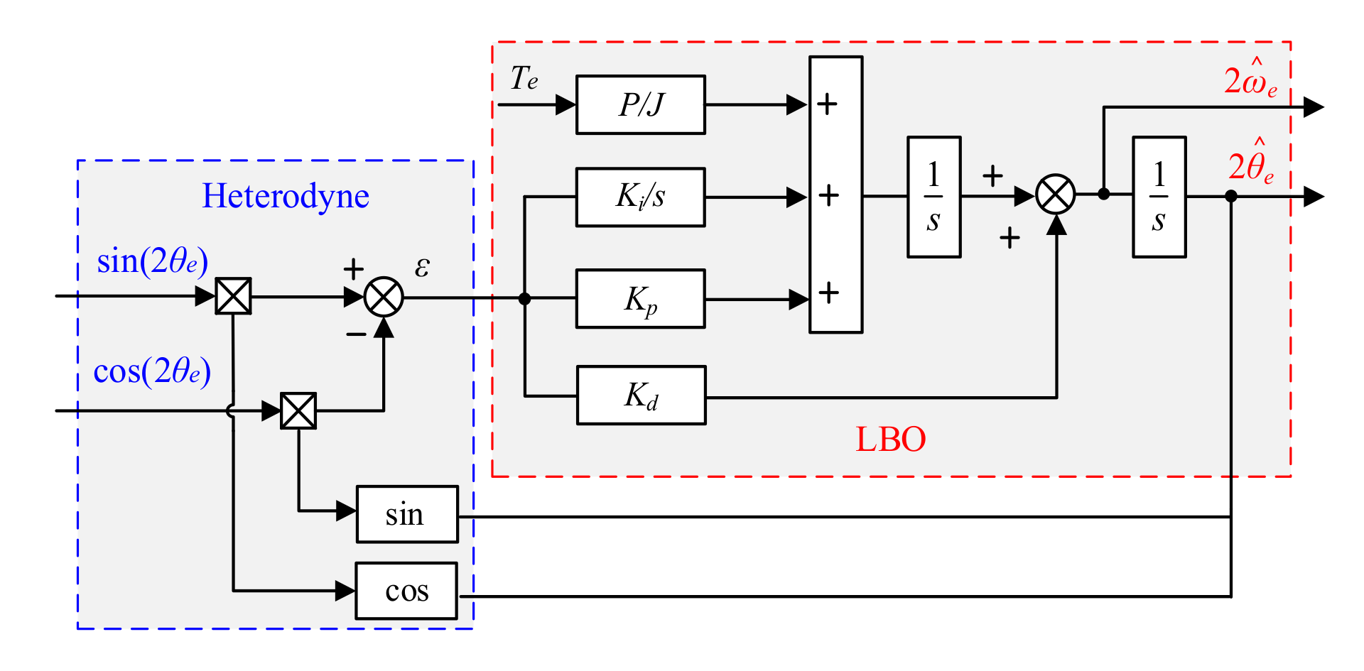
3.3. Luenberger-Based Observer Processing

The rotor position θ_e can be obtained from Equation (12). To solve the problem, as stated in Section 2.2, a Luenberger-based observer (LBO) [32] is proposed and designed from the motor’s mechanical characteristic.

The block diagram of the LBO observer is shown in Figure 7. Through the heterodyne method, the position tracking error signal ε is calculated by the sine and cosine signals which contain the position information. Then, the signal ε is passed through the LBO. It is designed to be a linear observer that filters out signal noise through the PID, where K_p, K_i, and K_d are the coefficients of the PID, respectively, to adjust the observer performance.

The transfer function of the observer can be expressed as

$$G\left(s\right)=\frac{J{K}_d{s}^2+P{K}_{p}s+P{K}_i}{J{s}^3+J{K}_d{s}^2+P{K}_{p}s+P{K}_i}$$

(21)

where J is the inertia moment of the IPMSM, P is the logarithm of the motor pole. The characteristic equation of the observer is

$$s^3+K_d{s}^2+\frac{P{K}_p}{J}s+\frac{P{K}_i}{J}=0$$

(22)

In order to adjust the parameters of the PID regulator, the three poles of the configuration Equation (22) are set to the same value, that is, the triple pole. At this time, the PID parameter can be represented by the pole

$$K_p=3J{\alpha }^2/P, K_i=-J{\alpha }^3/P, K_d=-3\alpha$$

(23)

where α is the triple pole.

Figure 8 shows the Bode diagram of the transfer function when the triple poles α take −5, −10, and −15 from top to bottom. As can be seen from the Bode diagram, the response speed is different when the poles select different values. When the response speed is high, the noise suppression capability is low. Therefore, different poles should be chosen according to the actual situation. Its stability is only related to the parameter configuration. If α is on the left side of the complex plane, that is, the value of α is negative, the observer is in a steady state. Therefore, this LBO has sufficient dynamic anti-interference ability.

Figure 9 shows the overall structure of the full-order SMO, which is based on SFT filter and LBO for the application of IPMSM sensorless speed control. The sign function is replaced by the saturation function to eliminate the chattering problem of the second-order SMO. The full-order SMO is employed to eliminate the use of the LPF. This improves the accuracy of the rotor position. To eliminate harmonics due to uncertainties, SFT filters is used.

According to the analysis in Section 3.3, the harmonic components in the estimated back EMF directly affect the accuracy of rotor position estimation. For this reason, two SFT functions are used to filter out higher harmonics. It can also be seen from Figure 9 that the reference signal of the SFT is generated by the estimated rotor position which obtained using the output of the LBO. These two feedback paths then return the reference signal from the LBO output to the SFT. Thus, this method eliminates the influence of torque ripple on harmonic components and can estimate the back-EMF accurately.

3.4. Phase Compensation Design

As can be seen from Figure 5b, different ω_c results in different filtering effect of the SFT function. In order to achieve better results, ω_c should be selected to be small. However, this will increase the phase delay caused by the filter. Therefore, it is necessary to design phase compensation. The phase compensation design is shown in Figure 9. Firstly, the component of E_ex containing the position information is obtained. Then, the higher harmonics are filtered by two SFT functions, and the obtained signal serves as the input to the position observer of LBO. The phase error caused by the filter can be compensated by the PI link. In addition, the position observer uses the LBO. It can also filter out high-frequency noise.

In view of the above analysis, the control method can accurately estimate the rotational speed and rotor position of the motor.

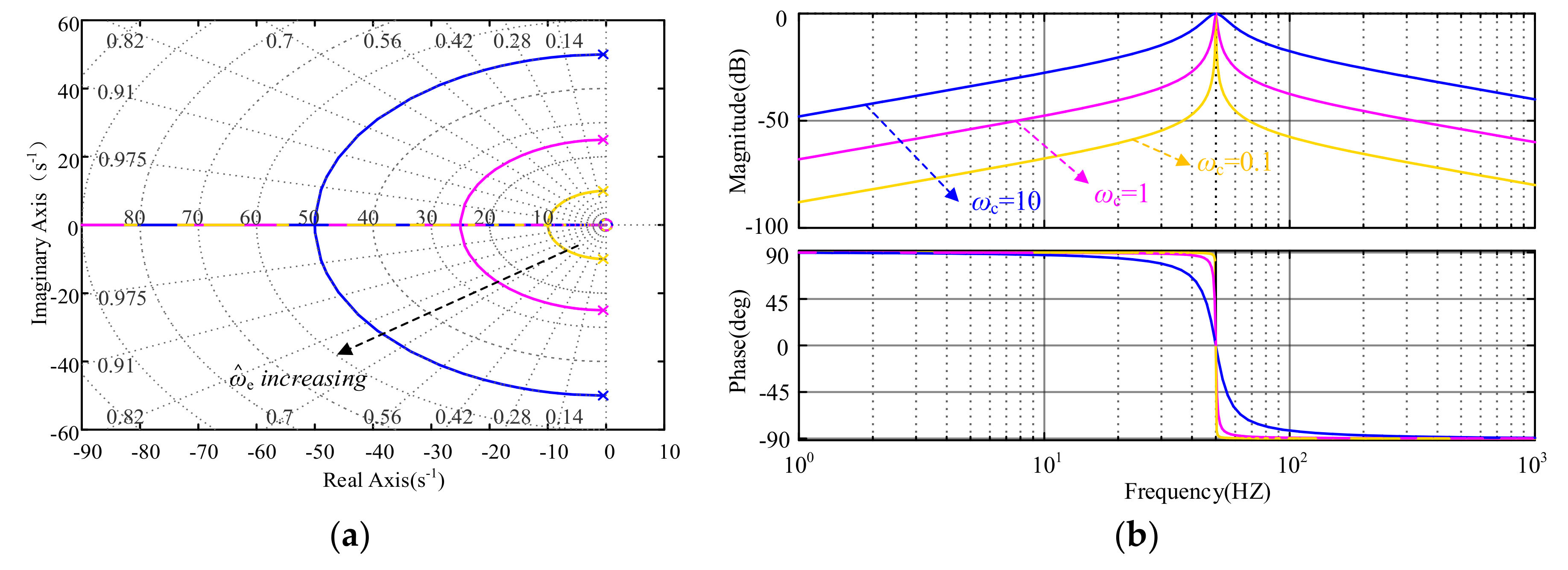
3.5. Stability Analysis of the Speed Observer System

The speed estimation observer system contains a full-order SMO, SFT Heterodyne and LBO, which are strongly coupled and are represented by Equations (24)–(27). Therefore, the system using full-order SMO, SFT heterodyne and LBO is a multi-input, multi-output system.

$$\frac{d}{dt}{\hat{\mathit{i}}}_s={\hat{\mathit{A}}\hat{\mathit{i}}}_s+\mathit{B}\mathit{u}+\mathit{C}\left(\hat{\mathit{e}}+\mathit{z}\right)$$

(24)

$$F_{\alpha /\beta }(s)=\frac{{\tilde{\widehat{e}}}_{\alpha /\beta }}{{\widehat{e}}_{\alpha /\beta }}=K_{p1}+\frac{K_{r}s}{s^2+2{\omega }_{c}s+{(2\pi \widehat{f})}^2}$$

(25)

$$\epsilon =(-{\tilde{\widehat{e}}}_{\beta }\cdot \cos 2{\widehat{\theta }}_e+{\tilde{\widehat{e}}}_{\alpha }\cdot \sin 2{\widehat{\theta }}_e)$$

(26)

$$\frac{2{\widehat{\theta }}_{\mathrm{e}}}{\epsilon }=\frac{J{K}_d{s}^2+P{K}_{p}s+P{K}_i}{J{s}^3+J{K}_d{s}^2+P{K}_{p}s+P{K}_i}$$

(27)

where, ${\widehat{\omega }}_e=\frac{{\widehat{\omega }}_m\cdot 2\pi \cdot n_p}{60}$, ${\widehat{\theta }}_e={\displaystyle \int {\widehat{\omega }}_e}dt$, $\widehat{f}=k_f\cdot {\widehat{\omega }}_m/2\pi$,${\psi }_f$ is the flux of IPMSM. ${\dot{\overline{i}}}_{\alpha }$ is the derivative of ${\overline{i}}_{\alpha }$, ${\dot{\overline{i}}}_{\beta }$ is the derivative of ${\overline{i}}_{\beta }$. The (28) represents the subtraction stage.

$$\left\{\begin{array}{l}{\dot{\overline{i}}}_{\alpha }=-\frac{R_s}{L_s}{\overline{i}}_{\alpha }-\frac{1}{L_s}({\widehat{e}}_{\alpha }-e_{\alpha })\\ {\dot{\overline{i}}}_{\beta }=-\frac{R_s}{L_s}{\overline{i}}_{\beta }-\frac{1}{L_s}({\widehat{e}}_{\beta }-e_{\beta })\end{array}\right.$$

(28)

The α-β axis model for the IPMSM in the stationary reference frame is characterized by (29).

$$\frac{d}{dt}{\hat{\mathit{i}}}_s={\hat{\mathit{A}}\hat{\mathit{i}}}_s+\mathrm{Bu}+\mathit{C}\left(\hat{\mathit{e}}+\mathit{z}\right)$$

(29)

where

$$\begin{gathered} {\hat{\mathit{i}}}_s={\left[\begin{array}{cc}{\widehat{i}}_{\alpha }& {\widehat{i}}_{\beta }\end{array}\right]}^T,\hat{\mathit{e}}={\left[\begin{array}{cc}{\widehat{e}}_{\alpha }& {\widehat{e}}_{\beta }\end{array}\right]}^T,\mathit{z}=\left[\begin{array}{l}{z}_{\alpha }\\ z_{\beta }\end{array}\right]=K\left[\begin{array}{c}sign({\widehat{i}}_{\alpha }-i_{\alpha })\\ sign({\widehat{i}}_{\beta }-i_{\beta })\end{array}\right], \\ \hat{\mathit{A}}=-R_s/L_d\cdot \mathit{I}+{\widehat{\omega }}_e(L_d-L_q)/L_d\cdot \mathit{J},\mathit{D}=\left[\begin{array}{cc}l& 0\\ 0& l\end{array}\right]. \end{gathered}$$

To prove the proper stability of this adaptive speed observer system, the SFT should be made as the structure (30).

$$\frac{d}{dt}{\hat{\mathit{i}}}_s={\hat{\mathit{A}}\hat{\mathit{i}}}_s+\mathit{B}\mathit{u}+\mathit{C}\left(\hat{\mathit{e}}+\mathit{z}\right)-K$$

(30)

where $K=\left[\begin{array}{cc}{k}_e& 0\\ 0& k_e\end{array}\right]F$, ${\widehat{e}}_{\alpha \beta }={\widehat{\omega }}_m\left[\begin{array}{c}-\sin {\widehat{\theta }}_e\\ \cos {\widehat{\theta }}_e\end{array}\right]$.

The SFT is defined upon the proportion and resonance of the estimated back-EMF.

$$F={(\begin{array}{cc}{f}_1& f_2\end{array})}^T=k_{p1}\cdot {\widehat{e}}_{\alpha \beta }+\frac{k_r\cdot 2{\omega }_c}{{\widehat{e}}_{\alpha \beta }\cdot t+2{\omega }_c+{\displaystyle {\int }_0^t{\widehat{e}}_{\alpha \beta }dt}}$$

(31)

Then, one can obtain

$$\dot{F}=-k_{p1}\cdot \frac{R_s}{L_s}\cdot I\cdot {\widehat{e}}_{\alpha \beta }+\frac{1}{L_s}I\cdot {\widehat{e}}_{\alpha \beta }-K+k_r\cdot 2{\omega }_c\cdot \frac{d}{dt}(\frac{1}{{\widehat{e}}_{\alpha \beta }\cdot t+2{\omega }_c+{\displaystyle {\int }_0^t{\widehat{e}}_{\alpha \beta }dt}})$$

(32)

The Lyapunov function V is selected as

$$V=\frac{1}{2}{F}^{T}F$$

Based on mathematic theory, if the following equation is convergent, the Lyapunov function V is convergent as well [13,14].

$$V^{\prime }=\frac{1}{2}{F}^{T}F+\frac{{({\widehat{\omega }}_m-{\omega }_m)}^2}{2}$$

Assuming that the rotor angular speed is constant, the following equation can be derived

$$\dot{V^{\prime }}=\frac{1}{2}{F}^T\dot{F}+({\widehat{\omega }}_m-{\omega }_m){\dot{\widehat{\omega }}}_m$$

(33)

Substituting (21) and (22) into (23), the following equation can be obtained

$$\begin{array}{l}\dot{V^{\prime }}=({\widehat{\omega }}_m-{\omega }_m){\dot{\widehat{\omega }}}_m+\frac{1}{2}{F}^T[-k_{p1}\cdot \frac{R_s}{L_s}\cdot I\cdot {\overline{i}}_{\alpha \beta }+\frac{1}{L_s}I\cdot {\overline{e}}_{\alpha \beta }-K+k_r\cdot 2{\omega }_c\cdot \frac{d}{dt}(\frac{1}{{\overline{i}}_{\alpha \beta }\cdot t+2{\omega }_c+{\displaystyle {\int }_0^t{\overline{i}}_{\alpha \beta }dt}})]\\ =({\widehat{\omega }}_m-{\omega }_m){\dot{\widehat{\omega }}}_m+\left[k_{p1}\cdot {\overline{i}}_{\alpha \beta }{}^T+\frac{k_r\cdot 2{\omega }_c}{{\overline{i}}_{\alpha \beta }{}^T\cdot t+2{\omega }_c+{\displaystyle {\int }_0^t{\overline{i}}_{\alpha \beta }{}^{T}dt}}\right]\cdot [-k_{p1}\cdot \frac{R_s}{L_s}\cdot I\cdot {\overline{i}}_{\alpha \beta }+\frac{1}{L_s}I\cdot {\overline{e}}_{\alpha \beta }-K+k_r\cdot 2{\omega }_c\cdot \frac{d}{dt}(\frac{1}{{\overline{i}}_{\alpha \beta }\cdot t+2{\omega }_c+{\displaystyle {\int }_0^t{\overline{i}}_{\alpha \beta }dt}})]\end{array}$$

(34)

According to Lyapunov stability theory, in order for the system to converge [15,16], it can be derived that

$$\frac{F^T}{L_s}I\cdot {\widehat{e}}_{\alpha \beta }+({\widehat{\omega }}_m-{\omega }_m){\dot{\widehat{\omega }}}_m=0$$

(35)

$$F^T\left[-k_{p1}\cdot \frac{R_s}{L_s}\cdot I\cdot {\widehat{e}}_{\alpha \beta }-K+\right.\left.k_r\cdot 2{\omega }_c\cdot \frac{d}{dt}(\frac{1}{{\widehat{e}}_{\alpha \beta }\cdot t+2{\omega }_c+{\displaystyle {\int }_0^t{\widehat{e}}_{\alpha \beta }dt}})\right]<0$$

(36)

From the inequality (26), the AFTO parameter and back-EMF gains k_p1, k_r and k_e can be obtained

$$F^T\left[-k_{p1}\cdot \frac{R_s}{L_s}\cdot I\cdot {\widehat{e}}_{\alpha \beta }-k_{e}F\right.\left.k_r\cdot 2{\omega }_c\cdot \frac{d}{dt}(\frac{1}{{\widehat{e}}_{\alpha \beta }\cdot t+2{\omega }_c+{\displaystyle {\int }_0^t{\widehat{e}}_{\alpha \beta }dt}})\right]<0$$

(37)

The sufficient conditions to satisfy the inequality (37) are

$$F^T\left[2k_r{\omega }_c\cdot \frac{d}{dt}(\frac{1}{{\widehat{e}}_{\alpha \beta }\cdot t+2{\omega }_c+{\displaystyle {\int }_0^t{\widehat{e}}_{\alpha \beta }dt}})-k_{p1}\frac{R_s}{L_s}\cdot I\cdot {\widehat{e}}_{\alpha \beta }\right]<0$$

(38)

$$-k_e{F}^{T}F<0$$

(39)

Therefore, from the two inequalities (38) and (39), the k_p1, k_r, k_e, and ϕ can be obtained

$$k_{p1}>0, k_r<\frac{k_{p1}\cdot R_s}{2{\omega }_c\cdot L_s}, k_e> 0$$

Through stability analysis, as long as the parameters meet k_p2 = 8.06, k_i = 16.25 and k_p1 > 0, and k_e > 0. when k_p1 = 10, k_r < 540, the whole adaptive velocity observer system is stable.

4. Simulation and Experimental Results of the Proposed Method

4.1. Simulation Results

Simulation results verify the correctness of the proposed method. Table 1 lists the IPMSM parameters for the test. MATLAB/Simulink was used to simulate the sensorless algorithm. In the simulation, the given motor speed is 1000 rpm.

Figure 10 shows the simulation results of the proposed full-order SMO sensorless control method based on the SFT filter and LBO for an IPMSM. Figure 10a shows the actual and estimated speed. The estimated speed follows the actual speed well. The harmonic content is significantly reduced compared with Figure 3a. The estimated rotational speed error is small, within ±0.1 rpm. The actual position of the rotor and the estimated one is compared in Figure 11.

Compared with Figure 3b, the estimated rotor position has no chattering phenomenon and the accuracy of the position estimation is clearly improved. The harmonics in the rotor position are eliminated as well. The rotor position estimation error is shown in Figure 10c. The error is finally stabilized at around 0.32°, and the error is significantly reduced. Figure 10d illustrates the observed extended back-EMF component. The observed back-EMF is smooth and free of harmonics, which ensures a high-precision estimation of the rotor position. Figure 10e provides the FFT analysis results of estimated back-EMF. Compared with the Figure 3e, the 3rd harmonic has been eliminated, and the 5th and 7th harmonics are also allocated to a negligible extent. The effectiveness of the proposed full-order SMO sensorless control method is verified by simulation results.

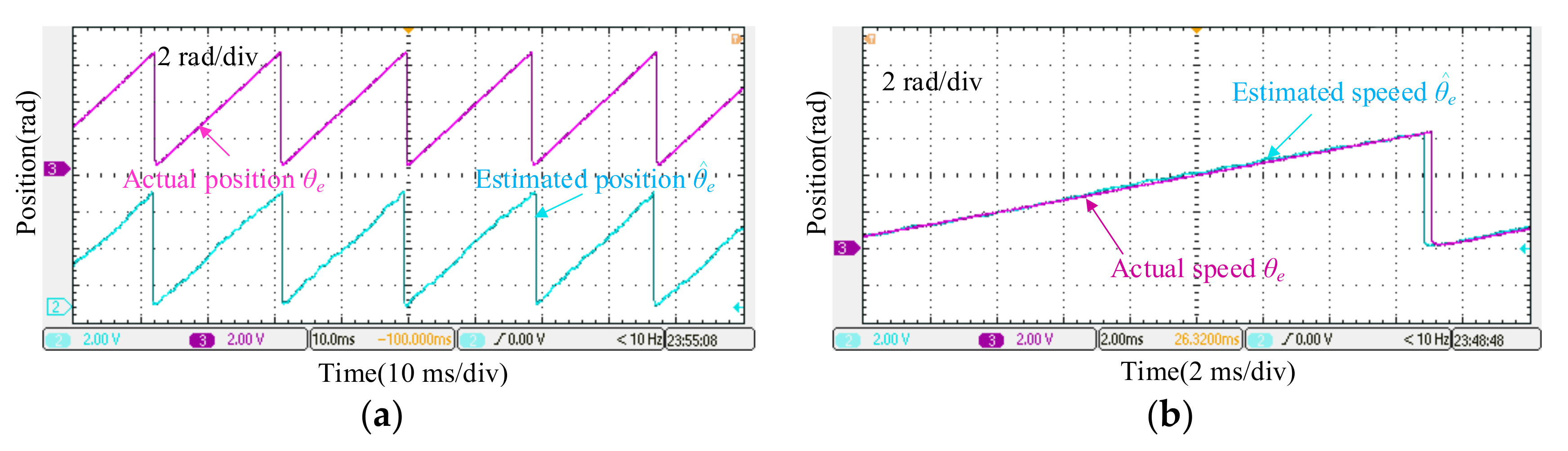
4.2. Experimental Results

The photo of experimental platform is shown in Figure 11. For the power drive circuit, six complementary PWM signals generated by dSPACE are used to drive the IPMSM. In addition, the power drive circuit also contains DC bus voltage acquisition circuit, stator current sampling circuit and overvoltage protection circuit. The stator current is detected by the CS040GT Hall current sensor. In SFT, the cutoff frequency ω_c set as 2. The control petameters of the phase compensation are k_p = 0.1 and k_i = 1.

Figure 12 and Figure 13 illustrate the experimental results of the actual speed and estimated position and speed employing the traditional second-order SMO method when the rotor speed runs from 0 rpm to 800 rpm and decrease to 0 rpm.

Figure 12 shows the experimental results of the actual speed and estimated speed employing the traditional second-order SMO method. Figure 12a gives the separated waveform. Figure 12b presents the overlapped waveforms. It can be seen from Figure 12a,b the estimated speed contains a large number of high-frequency harmonic components. The pulsation of the estimated speed is ±40 rpm.

The experimental results of the actual and estimated rotor angular position by the traditional second-order SMO method is shown in Figure 13a,b. Figure 13b presents the existence of a clear delay between the actual and estimated rotor positions. The phase delay caused by LPF of the traditional SMO method, which is also the main reason for its low positional accuracy.

Figure 14 and Figure 15 give the experimental results of the speed and rotor position using the proposed full-order SMO method based on SFT filter when the rotor speed was changed from 0 to 800 rpm and 0 rpm. The experimental results of the actual speed and estimated speed is present in Figure 14. Figure 14a gives the separated waveform and Figure 14b presents the overlapped waveforms. Compared with the traditional second-order SMO method, the high harmonics of the motor are good, and the rotor speed has no obvious pulsation, which is basically coincident with the actual rotor speed, and the errors between the actual speed and estimated speed are within ±5 rpm.

Figure 15a,b illustrate the experimental results of the rotor position using the proposed full-order SMO method based on the SFT filter. Since there is no LPF used in the full-order SMO, the phase delay is reduced. The rotor position error is within 5°. In addition, the SFT filter can filter out the harmonics caused by the nonlinearity of the inverter. The phase error caused by LPF is eliminated by the compensation link. In addition, high harmonics can be filtered out by the LBO. Therefore, the harmonic in the estimated rotor position can be eliminated.

Figure 16 shows the estimated back-EMFs by the full-order SMO method based on the SFT filter. It can be seen that the harmonics in the estimated back-EMF are significantly reduced. The waveforms of the estimated back-EMFs are smooth, which ensures a high-precision estimation of the rotor position.

Figure 17 shows the experimental results for the estimated and actual rotor angular positions and speed employing the proposed method when the rotor speed was 3000 rad/min. The estimation errors were ±6 rad/min when the speed was 3000 rad/min, respectively.

5. Conclusions

This paper proposes a sensorless, SFT-based, full-order SMO method for employ in IPMSM drive applications of the medium- and high-speed sensorless control strategy. Considering the harmonic influence of the inverter nonlinearity on the traditional method, this method uses a full-order SMO to replace the traditional second-order SMO to avoid the phase delay defects caused by the use of filters. On this basis, the SFT function is used to filter the observed extended back-EMF signal. By tracking the current changing stator current and filtering out the harmonics that are not part of the tracking signal, the static tracking of the stator current is achieved. The experimental results have proved that the estimated rotor position and the harmonic content in the rotor speed are significantly reduced, and the rotor position error is significantly reduced.

References

1. Gokasan, M.; Bogosyan, S.; Goering, D. Sliding mode based powertrain control for efficiency improvement in series hybrid-electric vehicles. IEEE Trans. Power Electron. 2006, 21, 779–790. [Google Scholar] [CrossRef] [Green Version]
2. Melfi, M.J.; Evon, S.; McElveen, R. Induction versus permanent magnet motors. IEEE Ind. Appl. Mag. 2009, 15, 28–35. [Google Scholar] [CrossRef]
3. Singh, S.; Tiwari, A.N. Various techniques of sensorless speed control of PMSM: A review. In Proceedings of the 2017 Second International Conference on Electrical, Computer and Communication Technologies (ICECCT), Coimbatore, India, 22–24 February 2017; pp. 1–6. [Google Scholar]
4. Liu, K.; Zhu, Z.Q. Quantum Genetic Algorithm-Based Parameter Estimation of PMSM under Variable Speed Control Accounting for System Identifiability and VSI Nonlinearity. IEEE Trans. Ind. Electron. 2014, 62, 2363–2371. [Google Scholar] [CrossRef]
5. Gao, Y.; Ehsani, M. Parametric design of the traction motor and energy storage for series hybrid off-road and military vehicles. IEEE Trans. Power Electron. 2006, 21, 749–755. [Google Scholar]
6. Lefebvre, G.; Gauthier, J.-Y.; Hijazi, A.; Lin-Shi, X.; Le Digarcher, V. Observability-Index-Based Control Strategy for Induction Machine Sensorless Drive at Low Speed. IEEE Trans. Ind. Electron. 2017, 64, 1929–1938. [Google Scholar] [CrossRef]
7. Pereira, W.C.A.; Oliveira, C.M.R.; Santana, M.P.; Almeida, T.E.P.; Castro, A.G.; Paula, G.T.; Aguiar, M.L. Improved Sensorless Vector Control of Induction motor Using Sliding Mode Observer. IEEE Lat. Am. Trans. 2016, 14, 3110–3116. [Google Scholar] [CrossRef]
8. Yang, S.; Li, X.; Ding, D.; Zhang, X.; Xie, Z. Speed sensorless control of induction motor based on sliding-mode observer and MRAS. In Proceedings of the 2016 IEEE 8th International Power Electronics and Motion Control Conference (IPEMC-ECCE Asia), Hefei, China, 22–26 May 2016; pp. 1889–1893. [Google Scholar]
9. Utkin, V.I.; Guldner, J.; Shi, J. Sliding Mode Control in Electro-Mechanical Systems; Taylor & Francis Group: New York, NY, USA, 2009. [Google Scholar]
10. Lee, K.; Choy, I.; Back, J.; Choi, J. Disturbance observer based sensorless speed controller for PMSM with improved robustness against load torque variation. In Proceedings of the 8th International Conference on Power Electronics—ECCE Asia, Jeju, Korea, 30 May–3 June 2011; pp. 2537–2543. [Google Scholar]
11. Hu, J.; Zou, J.; Xu, F.; Li, Y.; Fu, Y. An Improved PMSM Rotor Position Sensor Based on Linear Hall Sensors. IEEE Trans. Magn. 2012, 48, 3591–3594. [Google Scholar] [CrossRef]
12. Weber, A.R.; Steiner, G. An accurate identification and compensation method for nonlinear inverter characteristics for ac motor drives. In Proceedings of the 2012 IEEE International Instrumentation and Measurement Technology Conference Proceedings, Graz, Austria, 13–16 May 2012; pp. 821–826. [Google Scholar]
13. Edwards, C.; Shtessel, Y.B. Adaptive Continuous Higher Order Sliding Mode Control. Automatica 2016, 65, 183–190. [Google Scholar] [CrossRef] [Green Version]
14. Roy, S.; Baldi, S.; Fridman, L.M. On adaptive sliding mode control without a priori bounded uncertainty. Automatica 2020, 111, 108650. [Google Scholar] [CrossRef]
15. Shtessel, Y.B.; Taleb, M.; Plestan, F. A novel adaptive-gain supertwisting sliding mode controller: Methodology and application. Automatica 2012, 48, 759–769. [Google Scholar] [CrossRef]
16. Roy, S.; Roy, S.B.; Lee, J.; Baldi, S. Overcoming the Underestimation and Overestimation Problems in Adaptive Sliding Mode Control. IEEE/ASME Trans. Mechatron. 2019, 24, 2031–2039. [Google Scholar] [CrossRef] [Green Version]
17. Bedetti, N.; Calligaro, S.; Petrella, R. Accurate modeling, compensation and self-commissioning of inverter voltage distortion for high-performance motor drives. In Proceedings of the 2014 IEEE Applied Power Electronics Conference and Exposition—APEC 2014, Fort Worth, TX, USA, 16–20 March 2014; pp. 1550–1557. [Google Scholar]
18. Wang, T.; Zhang, H.; Gao, Q.; Xu, Z.; Li, J.; Gerada, C. Enhanced Self-Sensing Capability of Permanent-Magnet Synchronous Machines: A Novel Saliency Modulation Rotor End Approach. IEEE Trans. Ind. Electron. 2016, 64, 3548–3556. [Google Scholar] [CrossRef]
19. Kumar, K.V.K.S.S.; Rao, B.V.; Kumar, G.V.E.S. Fractional order PLL based sensorless control of PMSM with sliding mode observer. In Proceedings of the 2018 International Conference on Power, Instrumentation, Control and Computing (PICC), Thrissur, India, 18–20 January 2018; pp. 1–6. [Google Scholar]
20. Song, X.; Fang, J.; Han, B.; Zheng, S. Adaptive Compensation Method for High-Speed Surface PMSM Sensorless Drives of EMF-Based Position Estimation Error. IEEE Trans. Power Electron. 2016, 31, 1438–1449. [Google Scholar] [CrossRef]
21. Jung, S.-H.; Kobayashi, H.; Doki, S.; Okuma, S. An improvement of sensorless control performance by a mathematical modelling method of spatial harmonics for a SynRM. In Proceedings of the 2010 International Power Electronics Conference—ECCE&ASIA, Sapporo, Japan, 21–24 June 2010; pp. 2010–2015. [Google Scholar]
22. Bao, D.; Wang, Y.; Pan, X.; Wang, X.; Li, K. Improved sensorless control method combining SMO and MRAS for surface PMSM drives. In Proceedings of the 2017 IEEE Industry Applications Society Annual Meeting, Cincinnati, OH, USA, 1–5 October 2017; pp. 1–5. [Google Scholar]
23. Shi, Y.; Sun, K.; Huang, L.; Li, Y. Online Identification of Permanent Magnet Flux Based on Extended Kalman Filter for IPMSM Drive With Position Sensorless Control. IEEE Trans. Ind. Electron. 2012, 59, 4169–4178. [Google Scholar] [CrossRef]
24. Auger, F.; Hilairet, M.; Guerrero, J.M.; Monmasson, E.; Orlowska-Kowalska, T.; Katsura, S. Industrial Applications of the Kalman Filter: A Review. IEEE Trans. Ind. Electron. 2013, 60, 5458–5471. [Google Scholar] [CrossRef] [Green Version]
25. Underwood, S.J.; Husain, I. Online Parameter Estimation and Adaptive Control of Permanent-Magnet Synchronous Machines. IEEE Trans. Ind. Electron. 2010, 57, 2435–2443. [Google Scholar] [CrossRef]
26. Liu, K.; Zhu, Z.-Q.; Stone, D.A. Parameter estimation for condition monitoring of PMSM stator winding and rotor permanent magnets. IEEE Trans. Ind. Electron. 2013, 60, 5902–5913. [Google Scholar] [CrossRef] [Green Version]
27. Luo, X.; Shen, A.; Cao, W.; Rao, W. Full order state observer of stator flux for permanent magnet synchronous motor based on parameter adaptive identification. In Proceedings of the 2013 IEEE 8th Conference on Industrial Electronics and Applications (ICIEA), Melbourne, Australia, 19–21 June 2013; pp. 1456–1461. [Google Scholar]
28. Chan, T.F.; Wang, W.; Wong, Y.K.; Borsje, P.; Ho, S.L. Sensorless permanent-magnet synchronous motor drive using a reduced-order rotor flux observer. IET Electr. Power Appl. 2008, 2, 88–98. [Google Scholar] [CrossRef]
29. Bao, D.; Pan, X.; Wang, Y.; Wang, X.; Li, K. Adaptive Synchronous-Frequency Tracking-Mode Observer for the Sensorless Control of a Surface PMSM. IEEE Trans. Ind. Appl. 2018, 54, 6460–6471. [Google Scholar] [CrossRef]
30. Wang, G.; Zhan, H.; Zhang, G.; Gui, X.; Xu, D. Adaptive Compensation Method of Position Estimation Harmonic Error for EMF-Based Observer in Sensorless IPMSM Drives. IEEE Trans. Power Electron. 2013, 29, 3055–3064. [Google Scholar] [CrossRef]
31. Bernard, P.; Praly, L. Robustness of rotor position observer for permanent magnet synchronous motors with unknown magnet flux. IFAC-Pap. 2017, 50, 15403–15408. [Google Scholar] [CrossRef]
32. He, L.; Wang, F.; Wang, J.; Rodriguez, J.A. Zynq Implemented Luenberger Disturbance Observer Based Predictive Control Scheme for PMSM Drives. IEEE Trans. Power Electron. 2019, 35, 1770–1778. [Google Scholar] [CrossRef]
Figure 1. The physical model of interior permanent-magnet synchronous motor (IPMSM).
Energies 13 06511 g001
Figure 2. Traditional second-order sliding mode observer (SMO) schematic.
Energies 13 06511 g002
Figure 3. The simulation results of estimated extended back-EMF by the traditional second-order SMO sensorless control method for an IPMSM. (a) The actual speed n and the estimated speed; (b) the actual position of the rotor θe and the estimated position; (c) the actual position of the rotor θe and the estimated position; (d) the rotor position error waveform; (e) the extended back-EMF component of the rotor position information observed by the traditional second-order SMO; (f) the harmonic spectrum obtained by FFT.
Energies 13 06511 g003aEnergies 13 06511 g003b
Figure 4. Schematic diagram of the SFT filter.
Energies 13 06511 g004
Figure 5. Analysis of the SFT function. (a) The root of the SFT function when ωc is increased; (b) Bode diagram of the SFT function when ωc increases.
Energies 13 06511 g005
Figure 6. Bode plot of the SFT function when ω ^ e increases.
Energies 13 06511 g006
Figure 7. Overall block diagram of the position observer.
Energies 13 06511 g007
Figure 8. Bode diagram of LBO transfer function.
Energies 13 06511 g008
Figure 9. Overall structure of the SFT and LBO-based IPMSM sensorless speed control.
Energies 13 06511 g009
Figure 10. Analysis of estimated extended back-EMF by the SFT-based sensorless speed control method for an IPMSM. (a) Estimated and measured rotor speed; (b) Estimated and measured rotor position; (c) Rotor position estimation error; (d) Estimated back-EMF; (e) the FFT of estimated back-EMF.
Energies 13 06511 g010
Figure 11. The experimental platform based on dSPACE.
Energies 13 06511 g011
Figure 12. Actual speed and estimated speed employing the traditional second-order SMO method when the motor operates at 800 rpm (a) separated waveform; (b) overlapped waveforms.
Energies 13 06511 g012
Figure 13. Actual position and estimated position employing the traditional second-order SMO method when the motor operates at 800 rpm (a) separated waveform; (b) overlapped waveforms.
Energies 13 06511 g013
Figure 14. Actual speed and estimated speed employing the proposed full-order SMO method based on SFT filter when the motor operates at 800 rpm. (a) separated waveform; (b) overlapped waveforms.
Energies 13 06511 g014
Figure 15. Actual position and estimated position employing the proposed full-order SMO method based on SFT filter when the motor operates at 800 rpm (a) separated waveform; (b) overlapped waveforms.
Energies 13 06511 g015
Figure 16. Extended back-EMF component when the motor operates at 800 rpm.
Energies 13 06511 g016
Figure 17. The experimental results using the proposed method when the rotor speed was3000 rad/min. (a) the measured and estimated rotor positions, (b) the measured and estimated rotor speeds.
Energies 13 06511 g017