Experimental Platform for Evaluation of On-Board Real-Time Motion Controllers for Electric Vehicles

Abstract

Electric vehicles are considered to be a greener and safer means of transport thanks to the distinguished advantages of electric motors. Studies on this object require experimental platforms for control validation purpose. Under the pressure of research, the development of these platforms must be reliable, safe, fast, and cost effective. To practically validate the control system, the controllers should be implemented in an on-board micro-controller platform; whereas, the vehicle model should be realized in a real-time emulator that behaves like the real vehicle. In this paper, we propose a signal hardware-in-the-loop simulation system for electric vehicles that are driven by four independent electric motors installed in wheels (in-wheel motor). The system is elaborately built on the basis of longitudinal, lateral, and yaw dynamics, as well as kinematic and position models, of which the characteristics are complete and comprehensive. The performance of the signal hardware-in-the-loop system is evaluated by various open-loop testing scenarios and by validation of a representative closed-loop optimal force distribution control. The proposed system can be applied for researches on active safety system of electric vehicles, including traction, braking control, force/torque distribution strategy, and electronic stability program.

1. Introduction

In the time of energy and environment crisis, electric vehicles (EVs) have emerged as a remarkable solution for replacing gasoline transportation system, which mainly causes environmental issues. Moreover, EVs also bring to users safer and more enjoyable transport means. In the energy usage aspect, EVs have much higher efficiency than that of Internal Combustion Engine (ICE) vehicles. As in recent statistical researches, the plug-to-wheel efficiency of EVs is 73–90% as compared to 16–37% tank-to-wheel efficiency of ICE cars and, more interestingly, if all diesel vehicles are converted to electric ones, the CO${}_2$ emissions will be reduced by 80% [1,2]. For those reasons, EVs have become attractive to researchers worldwide.

Thanks to outstanding features of electric motors, EVs have opened various new research topics. Besides traditional but prospective studies on Power Electronics [3,4] and Electric Drives [5], there are many other subjects that are particularly oriented to EVs, for example, Motion Control [6], Energy Management System [7], and Autonomous Driving [8]. Motion control, also called an active safety system, has exploited the major advantages of electric motors installed on EVs very well. With very fast response (just a few milliseconds), electric cars can achieve better driving performance in comparison with ICE vehicles [9]. Furthermore, the compact and simple structure allow for the separate integration of traction motors into wheels that not only increase the flexible movement, but also increases many interesting studies on driving force distribution for four-wheel-driven vehicles [10,11,12,13].

The common point of all research resides on the fact that the control performance must be validated in some ways before prototyping. The best approach is to conduct experimental tests on a real vehicle. Such experiments can deliver the most convincing results and totally evaluate the whole system, i.e., the response of the control strategy to the internal state variations inside the vehicle as well as external influences from real operating environment. On the contrary, its drawbacks are also significant, namely high cost, time consuming, and even very dangerous to experimenters. Another approach for overcoming experimental difficulties is to simulate the entire system on a simulation software, e.g., Matlab/Simulink. Following this solution, a mathematical/numerical model of EVs must be developed [14,15,16]. Testing the control system on a software seems to be reasonable, as the model can be modified in order to adapt to various requirements and the validation can be freely performed as many times as needed without either harm or expenditure. However, yet, numerical simulation is still off-line test, i.e., the results are not validated in real-time, which restricts the evaluated control system to be applicable in real vehicles.

In order to fill the gap between validating the system by real-road experiments and that by off-line software, Hardware-In-the-Loop (HIL) Simulation System is the proper solution. HIL simulation is the technique that uses equivalent models to replace some real parts of the system, connect to the system-under-test, and then implement the experiment for control validation. Contrary to software simulation, the equivalent models are executed in real-time on a hardware platform that must be designed to be synchronously compatible with the entire studied system. For many years, HIL simulation has been used widely because of remarkable advantages. It offers a cost-effective solution for researches and shortens the time of control system development. Experiments on HIL system are safe and they can be repeated with exactly the same conditions, which is impossible or extremely difficult in real-road test.

Developing a HIL simulation system, in fact, is a challenging work. On one hand, it should precisely represent behavior and/or distinguishing features of the studied system, in which all physical principles must be obeyed. Moreover, the simulation system is necessarily designed in order to adapt to research purpose and be open for future works. On the other hand, the HIL system needs to be simple enough to feasibly implement in real-time due to limitations in computational capability of hardware platforms. Development expenditure is also an important factor that must be compromised with mentioned difficulties.

Currently, there are commercial simulation software that can simulate EVs and vehicle control systems, for example, CarSim [17] and veDYNA [18]. Research on EVs can be validated in real-time by these products, but with specific hardware that are supplied by the same company. Such solutions are plausible, because of the compatibility of the system, but, as a result, the investment for both hardware and software is also considerable.

In the literature, HIL systems are well worked out. There are several types of HIL simulation systems that depend on design purpose as well as which subsystem is replaced [19].

• Signal HIL Simulation. The purpose of this type is to validate the performance of the developed controller in actual operation. Whereas, the controlled system is simulated based on its mathematical model and implemented on a real-time platform [20]. In order to do that, the equivalent model must act with similar behaviors to what it simulates and, furthermore, the model should imitate the real system to make the controller "reckon" that it is working with a real process. On the controller side, the algorithm should be programmed and compiled in order to run on a chosen processing hardware with all interfaces designed as a real Electronic Control Unit (ECU).
• Power HIL Simulation consists of two types, including Full-scale and Reduced-scale power HIL simulation.

Full-scale power HIL system is used in order to validate a part (with control included) of the system before bringing into the real process. In the implementation of this type, the total system is broken down into subsystems. The subsystems-under-test are retained, while the ones are modeled by an equivalent power emulated system [21]. Additionally, the simulated power system is controlled in such a way that it has the same characteristics with the real part that it emulates. The Power HIL simulation is likewise suitable for testing a new subsystem and its control that will be embedded into the available system.

A reduced-scale power HIL system has the same principle with that of full-scale power HIL ones, but with the lower level of simulation power [22,23,24,25]. In other words, both the subsystem to be validated and the emulated model will be tested with reduced power in order to avoid the risk of damage. However, the controller for the system is still designed with full-power level to quickly transfer to real process with minimum programming effort. Accordignly, there are some gains that must be used on the signal into/out of the controller, which is called power adaptation as well.

Among this comprehensive classification, signal HIL system exposes some advantages that can be applied not only for vehicle simulation, but also for many other research fields, e.g process control [26], robotics [27], and power system [28]. This kind of HIL shows its dominant features in studies that operate at high power level and/or work in hazardous environments, with dangerous experimental conditions and high investment cost, because it uses numerical models for real-time simulation instead of real/power elements. For EV researches, signal HIL simulation is a proper way for representing the vehicle effectively. In [29], an electronic stability controller for vehicle was developed and tested on a signal HIL system, which achieved good results. Although the developed model of this work only focuses on lateral behavior, the benefit of the real-time simulation system was fully exploited. Some other studies aimed to build HIL system in a signal level in order to validate vehicle control units in several applications, such as for motion control purpose [30,31], for motor control and power supply evaluation [32], or for ECU development [33]. These works have taken into account many hardware platforms, including DS2210 of dSPACE, NI-PXI and CompactRIO of National Instruments. However, models in these researches are still simple, which could not highlight the complicated relationship in motion of EVs and, more importantly, they targeted the single/dual motor drivetrain configuration. Another study in [34] attempted to develop signal HIL system for multi-motor vehicle based on various hardware platforms and the data fusion approach. Nevertheless, the EV in this research is a multi-axle one and, for military purpose, not for passenger cars.

In this paper, we propose a novel experimental platform that is based on the concept of signal HIL simulation system for validation of motion control strategies of EVs in real-time. The proposed system has the following merits.

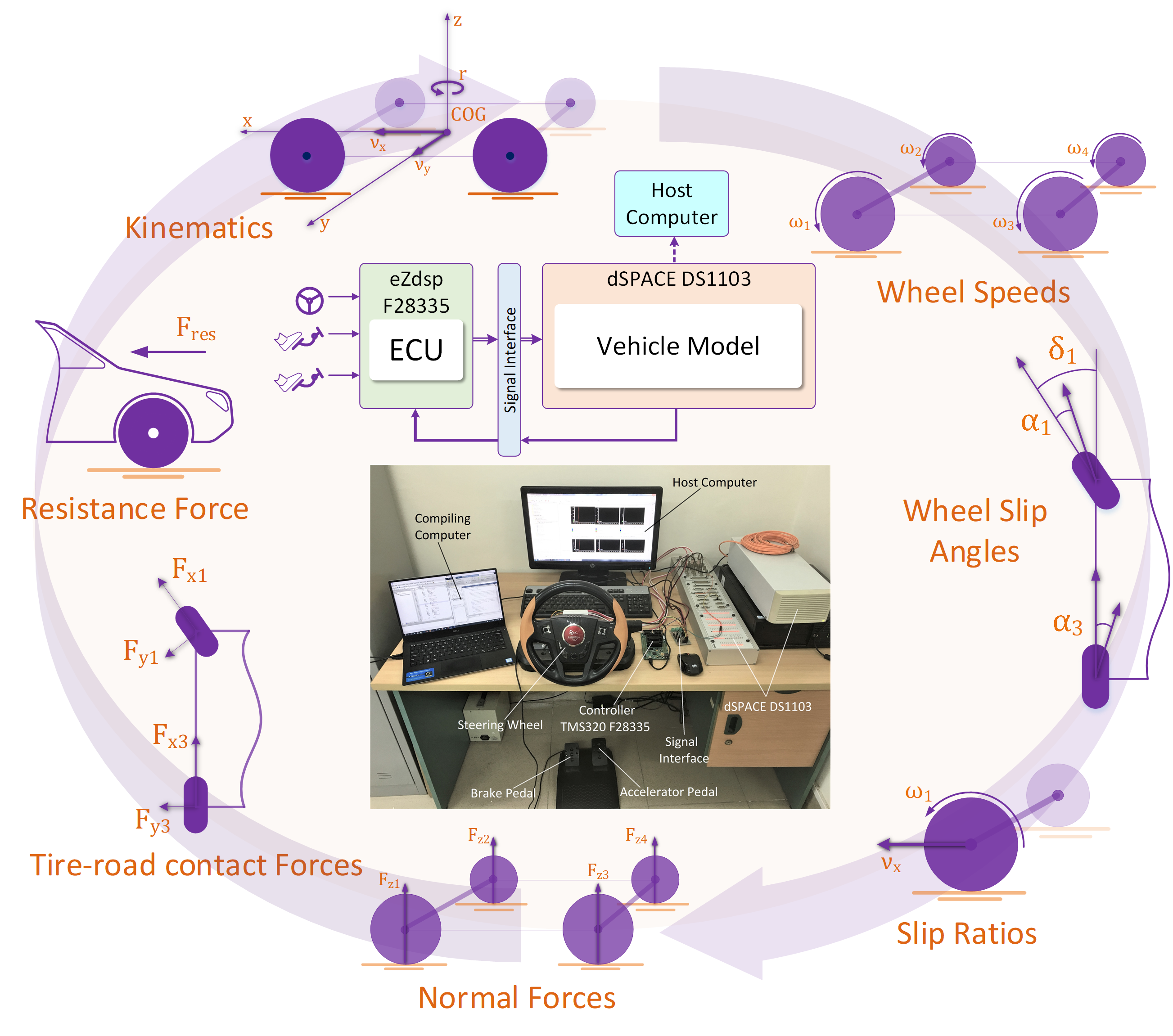
• The proposed system describes in details the dynamics and kinematics of four in-wheel-motors (4-IWM) EVs in both longitudinal and lateral motions, which are the typical moving directions used in motion control.
• The experimental platform of the paper is well fitted to the development of motion control systems, including traction/braking control, stability control, and driving force distribution strategy particularly for 4-IWM EVs.
• The signal HIL simulation system is built from available, common, and reasonable hardware platforms that encourages research on EVs as safer and greener means of transportation.

The performance of the proposed signal HIL system is evaluated by various testing scenarios. Additionally, an application example of a driving force distribution algorithm is deployed and validated on the proposed platform. All of the evaluation results demonstrate the advantages of the proposed approach.

The remain of the paper is organized, as follows. Section 2 describes the configuration and hardware deployment of the proposed platform. Section 3 develops the mathematical model of the studied EV. Section 4 presents the testing scenarios and evaluation results. Section 5 illustrates an application example on motion control of EVs that is implemented on the proposed signal HIL simulation system. Finally, Section 6 provides conclusions.

2. Experimental Platform Realization

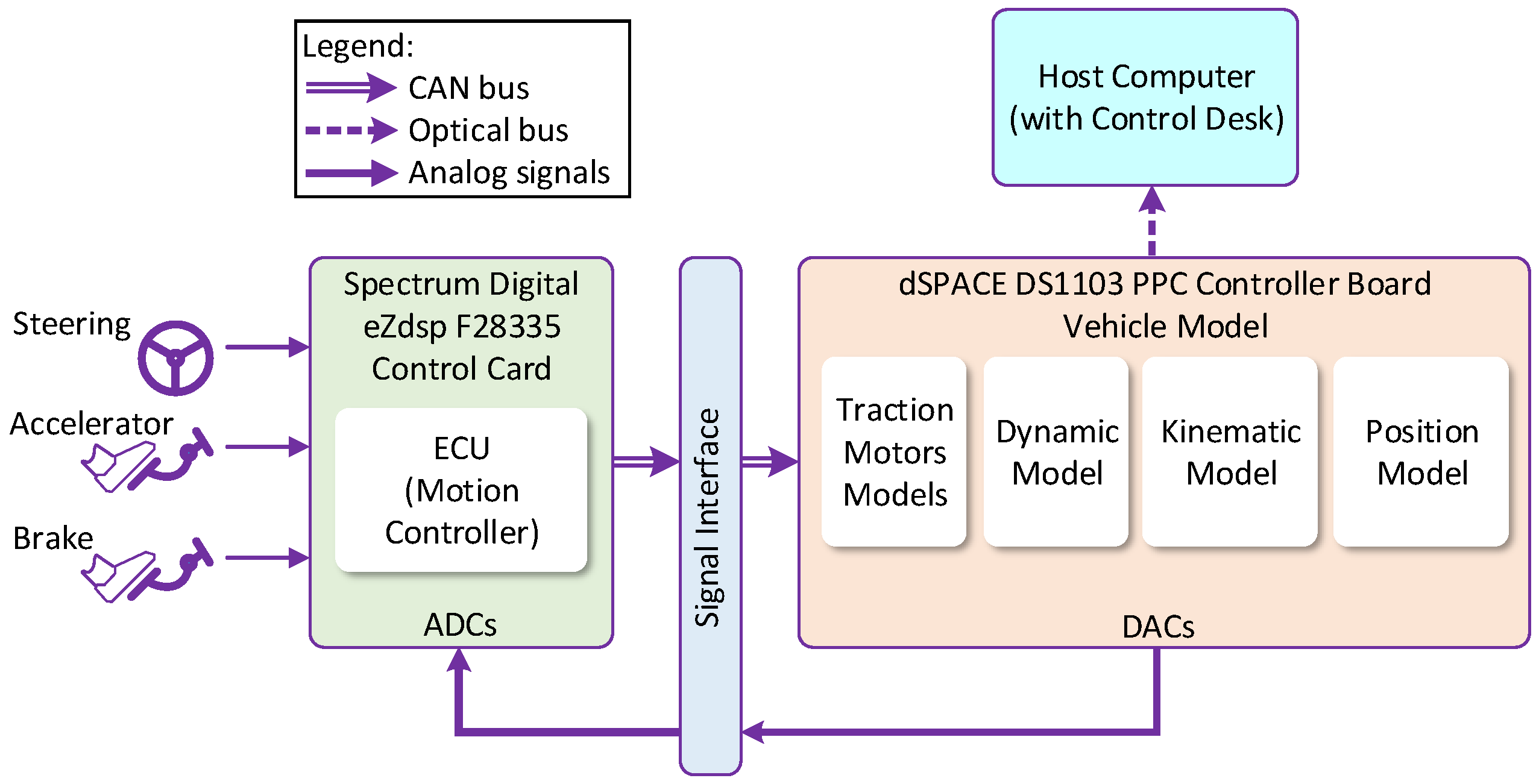
2.1. System Configuration

Generally, a non-autonomous moving vehicle consists of three main constituent entities, i.e., the driver, the control system, and the vehicle itself. The driver intervenes in the motion of the vehicle by giving his/her commands through the steering wheel, accelerator and brake pedals. The duty of the control system is to control the vehicle following the driver’s commands and simultaneously keep the vehicle and passengers in safe and comfort states. In order to carry out its job, besides receiving driver’s commands, the controller also observes states of the vehicle in order to generate appropriate control signals that are then sent to the traction system to make the movement.

Figure 1 illustrates the comprehensive system configuration, in which all of the entities will be modeled and simulated, including command signals from the driver, the control system, and the EV. Driver’s commands are represented by ${\delta }_{dr},T_{dr},T_{br}$ for the steering angle, the driving torque, and the braking torque, respectively, as shown in this figure. As the paper targets four-wheel independently driven vehicles, the control system will be in charge of two tasks, i.e., (i) adjust the commands that are received from the driver to anticipate appropriate total set-points for safety reasons of the vehicle and (ii) distribute these set-points to the traction motor control systems and the steering system based on a given allocation algorithm. Consequently, the outputs of the control system after the distribution algorithm are denoted by ${\delta }_i^{*}$ for distributed steering angle, $T_{di}^{*}$ for distributed driving torque, and $T_{bi}^{*}$ for distributed braking torque, in which the subscript $i=1..4$ with respect to wheels of the vehicle.

Eventually, the vehicle model will be divided into three parts, which are the powertrain of traction motors, the dynamic and the kinematic models. The position model that is based on longitudinal $v_x$ and lateral $v_y$ velocities are also described. It is noted that some other parts of the vehicle may not be mentioned in the figure, such as steering system, tire model because of the complexity in presentation, but the sophisticated relationship among all of the parts inside the vehicle will be described in detail later.

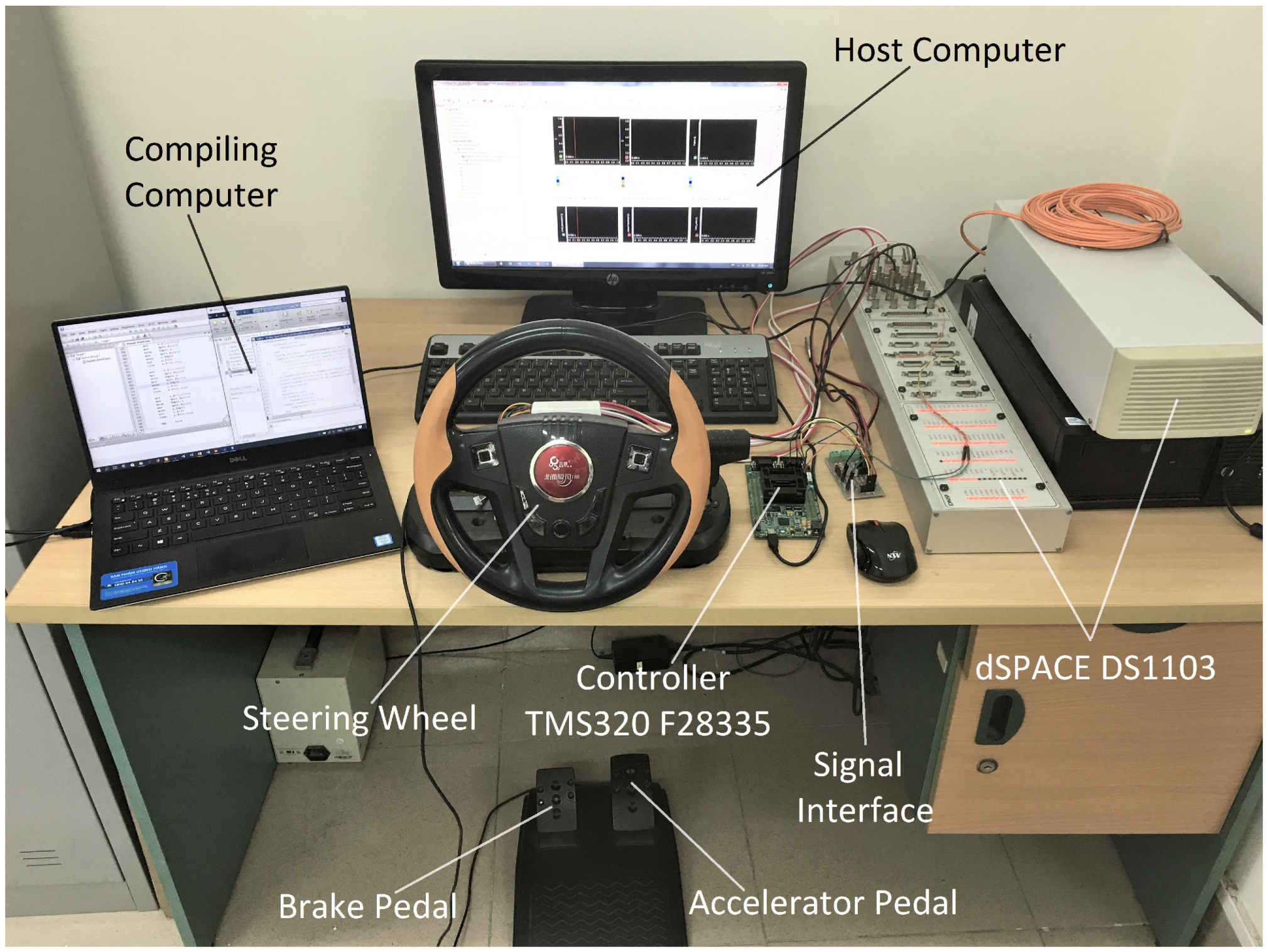
2.2. Hardware Realization

Based on the proposed configuration, Figure 2 illustrates the entire signal HIL simulation system in terms of hardware implementation. The HIL system adopts two control boards as the main hardware platforms, where each of them covers the specific tasks.

Firstly, the complete EV simulation model is adapted to run on DS1103 PPC Controller Board. This well-known multi-purpose research platform was designed by dSPACE with powerful computing capabilities and various I/O types. Some impressive specifications are 1GHz Central Processing Unit (CPU), 96 MB global SDRAM, 16 ADC channels with 16-bit resolution, 16 DAC channels also with 16-bit resolution, 32 parallel digital Inputs/Outputs (I/Os), and many supported communication protocols. Differently from the simulation on Matlab/Simulink, it should follow some steps for hardware implementation.

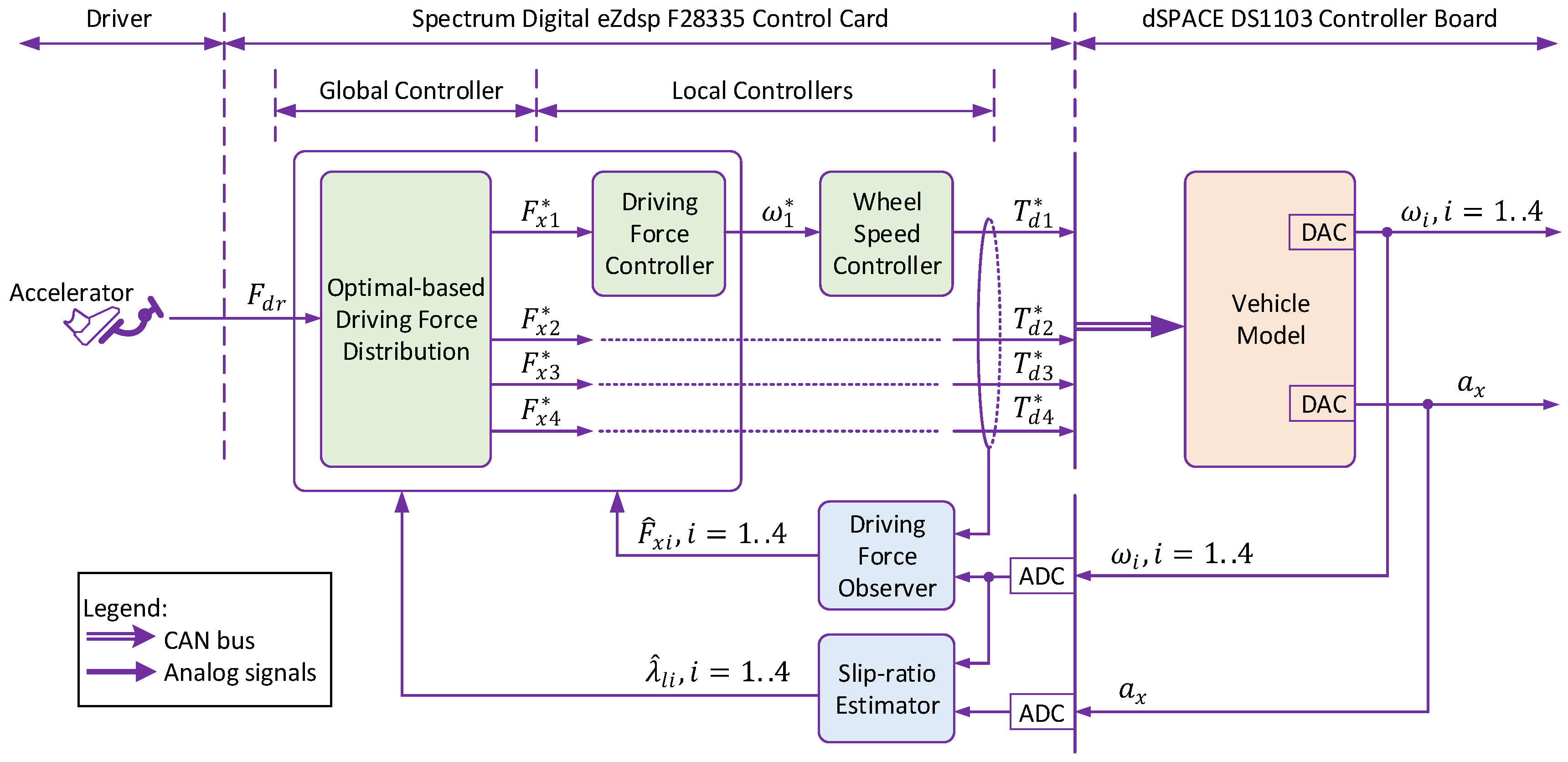
• All of the inputs and outputs of the model must be defined with proper I/Os of the DS1103. Unlike in the simulation, where all of the control signals as well as feedback information can be directly linked between the controller and the EV model, as illustrated in Figure 2 and referred to Figure 1, the control signals are transferred through CAN bus communication protocol, other states of the EV are converted into analog signals and exchanged among the platforms. Accordingly, such information must be assigned to appropriate hardware I/Os.
• Typically, the calculated values in the model are represented in floating-point data type, whereas the CAN bus protocol uses unsigned integer in its data field, therefore, data conversion should be taken into account not only for DS1103, but also for all hardware platforms.
• The sample time is the fundamental factor that needs to be carefully chosen. It is the constant iteration of time, in which all computations of the model are repeated. The smaller sample time is used, the more precise model will be but as a trade-off, the higher computational hardware may be required. In this paper, a sample time of 0.5 ms is used.
• After such preparation, the EV model can be complied and downloaded to deploy on the DS1103.

Secondly, the eZdsp F28335 Control Card from Spectrum Digital is used for the realization of the control algorithm, i.e., motion controller in this case. The core of the control card is the TMS320F28335 digital signal controller of Texas Instruments that offers the speed of 150 MHz with 32-bit floating point unit on chip. In the proposed HIL system, the eZdsp F28335 imitates the real ECU of the vehicle, which is responsible for the strategy of allocating command torque from driver to the separated motor controllers. In order to do the task, the ECU is connected to the driving system, including the steering wheel, the accelerator and brake pedals, and also collects measured physical data from the vehicle model. The distributed torque values and other control information can be transfer to the EV model on DS1103 through CAN bus. For that reasons, the implementation of control system onto this hardware platform has similar steps as that of DS1103. Based on the requirements of the control algorithm, the number of measured states may varies, so the quantity of analog-to-digital (ADC) and digital-to-analog (DAC) channels on both hardware platforms needs to be defined and assigned appropriately.

Because of different working voltage of the two hardware platforms, the signal interface is designed in order to harmonize the signals exchanged in the system and filter electromagnetic interference (EMI noise) as well. A host computer with installed Control Desk is used in order to collect and store the experimental data. This is the software that is provided together with the DS1103 for human-machine-interface (HMI) design and measurement data acquisition.

Eventually, the complete signal HIL simulation system is connected and described in Figure 3.

3. Mathematical Model of 4 In-Wheel-Motor Electric Vehicles

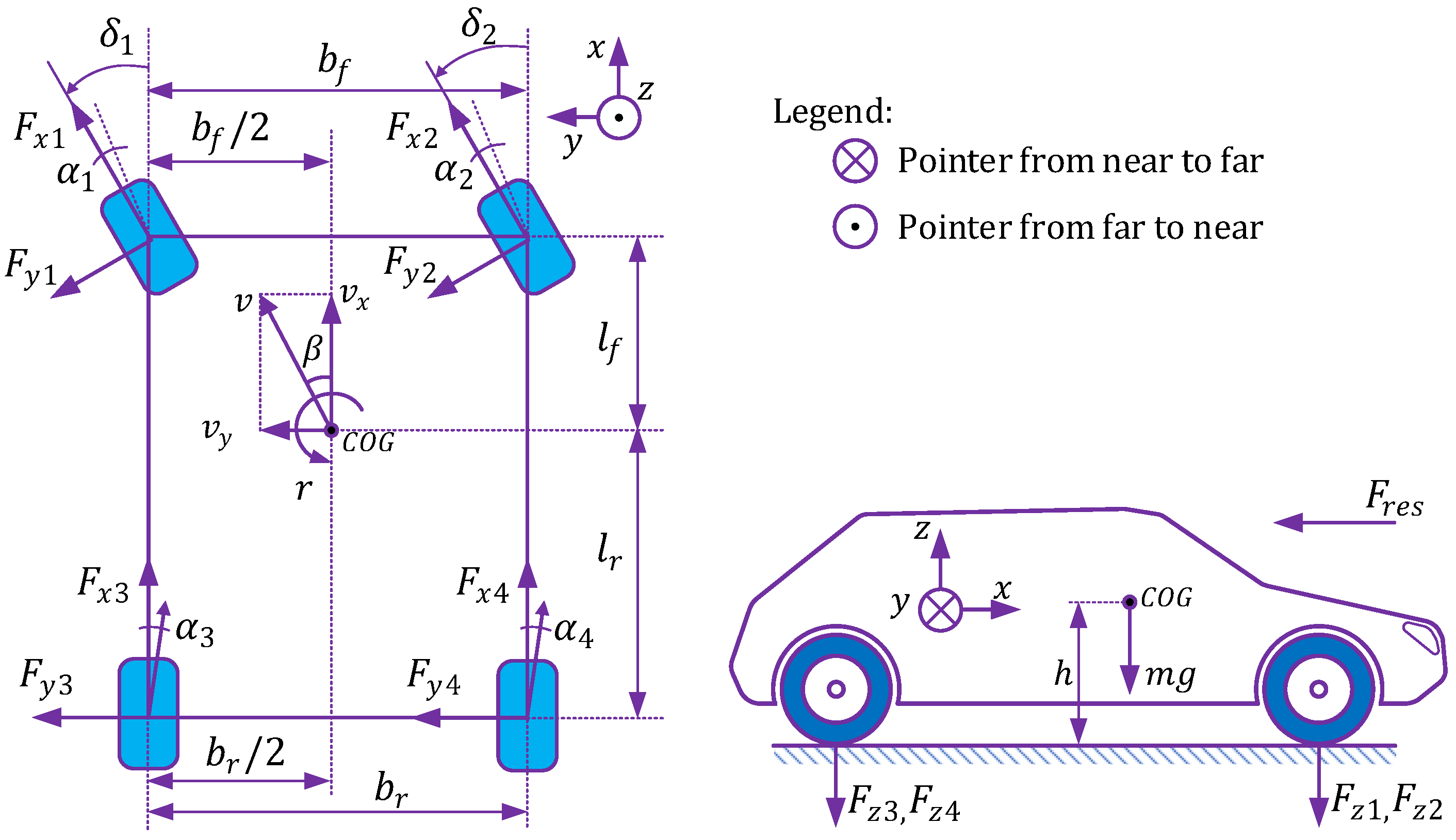
3.1. Vehicle Dynamic Model

A vehicle can be seen as a six degrees of freedom moving object. However, for reasons of simplicity, computational-effectiveness, as well as for representing common vehicles, some assumptions can be made, as follows.

• The vehicle adopts the two-front-wheel steering system. Therefore, both rear wheels are fixed at rear axle as non-steering ones.
• The vehicle is considered to be moving in longitudinal, lateral and yaw directions only, i.e., reduced to three degrees of freedom.

Figure 4 shows how forces apply to the vehicle body as well as wheels and other information related to motion, coordinate systems, and geometric parameters of the vehicle.

3.1.1. Force and Torque Balance Dynamic Model

A vehicle requires appropriate forces to be applied on wheels for its movement. The combination in amplitude of these forces decides the longitudinal behavior of the vehicle. Moreover, the coupling of different direction forces also creates a torque, which is incorporated with steering system to make the cornering and lateral behavior of the vehicle. Based on Figure 4 and Newton’s second law, the force balance equations in longitudinal and lateral directions and torque balance around vertical axis are written as in (1)

$$\begin{array}{cc}\hfill m{a}_x& =(F_{x1}cos{\delta }_1+F_{x2}cos{\delta }_2)-(F_{y1}sin{\delta }_1+F_{y2}sin{\delta }_2)+F_{x3}+F_{x4}-F_{res}\hfill \\ \hfill m{a}_y& =(F_{x1}sin{\delta }_1+F_{x2}sin{\delta }_2)+(F_{y1}cos{\delta }_1+F_{y2}cos{\delta }_2)+F_{y3}+F_{y4}\hfill \\ \hfill J_z\dot{r}& =(l_f{F}_{x1}sin{\delta }_1+l_f{F}_{x2}sin{\delta }_2)+(l_f{F}_{y1}cos{\delta }_1+l_f{F}_{y2}cos{\delta }_2)-l_r(F_{y3}+F_{y4})\hfill \\ \hfill & -0.5b_f(F_{x1}cos{\delta }_1-F_{x2}cos{\delta }_2)+0.5b_f(F_{y1}sin{\delta }_1-F_{y2}sin{\delta }_2)-0.5b_r(F_{x3}-F_{x4})\hfill \end{array}$$

(1)

where, m is the mass of the vehicle, $J_z$ indicates moment of inertia around z-axis, r denotes yaw rate, $F_{xi},F_{yi}$ are longitudinal and lateral forces applied at wheels, the subscript $i=1\dots 4$ denotes front-left, front-right, rear-left, and rear-right wheels respectively, $a_x,a_y$ are the acceleration of the vehicle in longitudinal and lateral directions, and parameters $l_f,l_r,b_f,b_r$ describe the geometric characteristic of the vehicle.

Equations in (1) are the dynamic model of the vehicle that contain various unknown variables. Therefore, the rest of this section will deliver all elements to complete the whole dynamic model, which fundamentally contributes to the proposed HIL system.

Neglecting the effect of wind, the total resistance force $F_{res}$ consists of air resistance force $F_{air}$ and rolling resistance force $F_{roll}$, and can be written, as follows [35].

$$F_{res}=F_{air}+F_{roll}=C_d{A}_F\frac{\rho }{2}{v}_x^2+c_{rr}mg$$

(2)

in which, $\rho$ is the air density, $A_F$ is the frontal area of the vehicle, $C_d$ is the aerodynamic drag coefficient, $c_{rr}$ denotes rolling friction coefficient, and g indicates the gravitational acceleration.

3.1.2. Steering Angle Distribution

As aforementioned assumptions, there are only two front wheels steered while cornering. It is common to convert the steering wheel position rotated by the driver to the effective steering angle of the front axle ${\delta }_{dr}$ generated by the rack and pinion system. In the other words, the model takes this effective steering angle as the driver’s command instead of steering wheel position into account.

When cornering with a given steering angle of ${\delta }_{dr}$, the center of gravity (COG) of the car will draw a circle whose radius R can be calculated by (3).

$$R=\sqrt{l_r^2+{(l_f+l_r)}^2{cot}^2{\delta }_{dr}}$$

(3)

However, because of the width of the axle, the two front wheels will move along two circles that have different radii from that of the CoG. If the steering angles of both wheels are assigned equally, then the vehicle might be unstable. For that reason, a distribution rule [36] can be used, as follows.

$$\left\{\begin{array}{c}\mathrm{if}{\delta }_{dr}>0\to {\delta }_1={\delta }_{dr},{\delta }_2=arctan{\displaystyle \frac{(R-0.5b_f)tan{\delta }_{dr}}{R+0.5b_f}}\hfill \\ \mathrm{if}{\delta }_{dr}<0\to {\delta }_2={\delta }_{dr},{\delta }_1=arctan{\displaystyle \frac{(R-0.5b_f)tan{\delta }_{dr}}{R+0.5b_f}}\hfill \\ \mathrm{if}{\delta }_{dr}=0\to {\delta }_1={\delta }_2={\delta }_{dr}\hfill \end{array}\right.$$

(4)

where, ${\delta }_1,{\delta }_2$ are the steering angles of the front-left and front-right wheels, respectively.

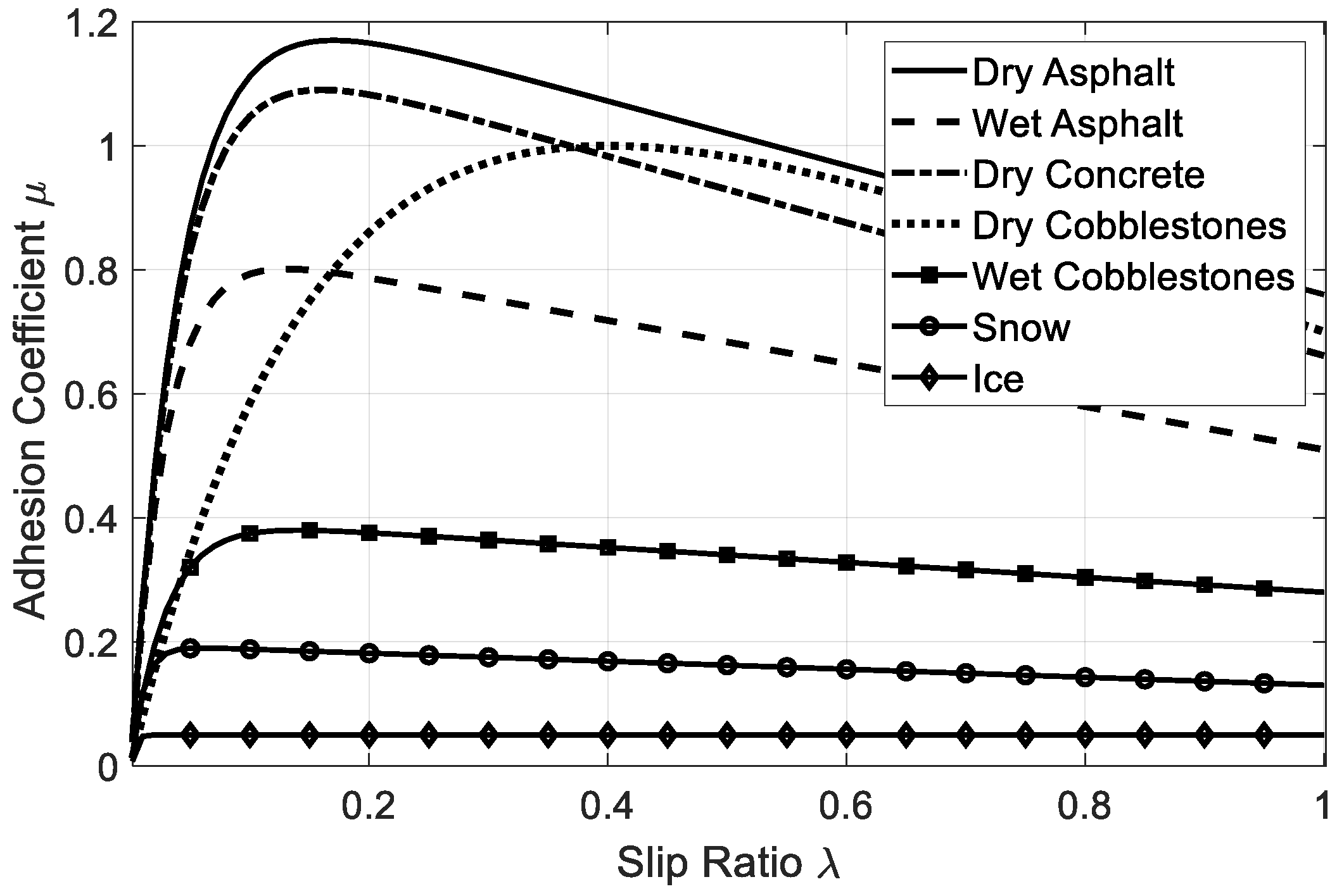
3.1.3. Tire-Road Behavior Model

Tire-road model describes the tire-road contact characteristic, which is represented by adhesion coefficient $\mu$ and its relationship to slip-ratio $\lambda$ of the vehicle. In the literature, this relationship is non-linear and it can be achieved from the famous Magic Formula [37] or other popular tire models, e.g., the Dugoff and LuGre friction model [38].

In this paper, the Burckhardt tire-road contact friction model is taken into account, since it has sufficient data set for various road types as compared to other mentioned ones. The $\mu -\lambda$ relationship at each wheel is given by Burckhardt, as follows.

$${\mu }_{res}=(c_1(1-e^{-c_2{\lambda }_{res}})-c_3{\lambda }_{res})e^{-c_4{\lambda }_{res}v}(1-c_5{F}_z^2)$$

(5)

where, ${\mu }_{res}$ is the adhesion coefficient at the tire-road contact, ${\lambda }_{res}$ is the slip-ratio of the considered wheel, $F_z$ denotes the normal force at a wheel of the vehicle, and $c_1-c_5$ are the road parameter sets. Each type of road has a specific characteristic and can be described by groups of parameters, as listed in

Table 1. Burckhard tire-road contact friction model parameter sets for typical road conditions.

Type of Road	${\mathit{c}}_{\mathbf{1}}$	${\mathit{c}}_{\mathbf{2}}$	${\mathit{c}}_{\mathbf{3}}$	${\mathit{c}}_{\mathbf{4}}$	${\mathit{c}}_{\mathbf{5}}$
Dry asphalt	1.2801	23.99	0.52	0.002–0.004	0.00015
Wet asphalt	0.857	33.822	0.347
Dry concrete	1.1973	25.168	0.5373
Dry cobblestone	1.3713	6.4565	0.6691
Wet cobblestone	0.4004	33.7080	0.12.4
Snow	0.1946	94.129	0.0646
Ice	0.05	306.39	0

, for typical road conditions. With respect to these data sets, the $\mu -\lambda$ relationship is shown in detail, as illustrated in Figure 5.

When cornering, the side force appears that causes the lateral motion of the vehicle. Therefore, the adhesion coefficient at each wheel is also divided into two components, as written in (6).

$$\begin{array}{cc}\hfill {\mu }_l& ={\mu }_{res}{\displaystyle \frac{{\lambda }_l}{{\lambda }_{res}}}\hfill \\ \hfill {\mu }_s& =k_s{\mu }_{res}{\displaystyle \frac{{\lambda }_s}{{\lambda }_{res}}}\hfill \end{array}$$

(6)

in which ${\mu }_l$ and ${\mu }_s$ are the adhesion coefficients in longitudinal and lateral directions, respectively, ${\lambda }_l$ and ${\lambda }_s$ are the slip ratio of the wheel in both of those orientations. In (6), $k_s$ is called attenuation factor, which has the value between 0.9 and 0.95 for low profile tires. Otherwise, $k_s$ is chosen as 1 [36].

3.1.4. Slip-Ratio Determination

Slip-ratio is a fundamental factor in motion control in order to guarantee the safety of a vehicle. In literature, the slip-ratio is the difference between velocity of the car and that of the wheel, which can be written in a simplified way, as follows.

$$\lambda ={\displaystyle \frac{\omega R_{eff}-v_x}{max(\omega R_{eff},v_x)}}$$

(7)

where, $R_{eff}$ is the effective radius of the wheel.

As mentioned in (6), the slip-ratio should be in various forms, which are listed in

Table 2. Longitudinal and lateral slip-ratio with respect to states of the vehicle.

Slip-Ratio	Braking ($\mathit{\omega }{\mathit{R}}_{\mathit{eff}}\mathbf{\le }{\mathit{v}}_{\mathit{W}}$)	Accelerating ($\mathit{\omega }{\mathit{R}}_{\mathit{eff}}\mathbf{>}{\mathit{v}}_{\mathit{W}}$)
${\lambda }_l$	${\displaystyle \frac{\omega R_{eff}cos\alpha -v_W}{v}}$	${\displaystyle \frac{\omega R_{eff}cos\alpha -v_W}{\omega R_{eff}cos\alpha }}$
${\lambda }_s$	${\displaystyle \frac{\omega R_{eff}sin\alpha }{v_W}}$	$tan\alpha$

where, $\alpha$ is the side-slip angle and $v_W$ is the longitudinal velocity of the specified wheel.

with respect to the orientations and accelerating/braking states of the vehicle.

Subsequently, the overall slip ratio is calculated as in (8).

$${\lambda }_{res}=\sqrt{{\lambda }_l^2+{\lambda }_s^2}$$

(8)

3.1.5. Wheel Longitudinal Velocity

A wheel longitudinal velocity $v_W$ is different from other velocities, e.g., vehicle velocity v, longitudinal velocity $v_x$, in some specific cases. When moving straight, all of the longitudinal velocities are identically the same in terms of value and orientation. However, when moving in a curve, depending on the tire-road contact adhesion feature, the direction of $v_W$ may not coincide with that of longitudinal axis of the wheel.

The longitudinal velocities of the wheels depend on geometric parameters and some other states of the car, and they can be approximated, as follows [36].

$$\begin{array}{cc}\hfill v_{W1}& =v-r(0.5b_f-l_f\beta )\hfill \\ \hfill v_{W2}& =v+r(0.5b_f+l_f\beta )\hfill \\ \hfill v_{W3}& =v-r(0.5b_r+l_r\beta )\hfill \\ \hfill v_{W3}& =v+r(0.5b_r-l_r\beta )\hfill \end{array}$$

(9)

where, $\beta$ is the body slip angle, as shown in Figure 4, and it can be determined as in (10).

$$\beta =arctan{\displaystyle \frac{v_y}{v_x}}$$

(10)

Additionally, the actual velocity at the COG of the vehicle can be obtained, as in (11).

$$v=\sqrt{v_x^2+v_y^2}$$

(11)

3.1.6. Side-Slip Angle Determination

The side-slip angle at a wheel is the one that describes the difference between longitudinal orientations of the wheel and its moving direction, as described in Figure 6. For front-wheel steering cars, the orientations of the front wheels are identically their steering angles. (12) shows the calculation of these slip angles based on the velocities of the vehicle.

$$\begin{array}{cc}\hfill {\alpha }_1& ={\delta }_1-arctan{\displaystyle \frac{v_y+l_{f}r}{v_x-0.5b_{f}r}}\hfill \\ \hfill {\alpha }_2& ={\delta }_2-arctan{\displaystyle \frac{v_y+l_{f}r}{v_x+0.5b_{f}r}}\hfill \\ \hfill {\alpha }_3& =-arctan{\displaystyle \frac{v_y-l_{r}r}{v_x-0.5b_{r}r}}\hfill \\ \hfill {\alpha }_4& =-arctan{\displaystyle \frac{v_y-l_{r}r}{v_x+0.5b_{r}r}}\hfill \end{array}$$

(12)

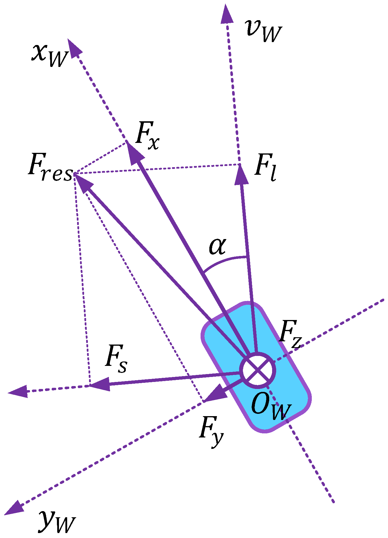
3.1.7. Forces Acting on a Wheel

It is the difference between the actual moving direction of the wheel $v_W$ and longitudinal axis of the wheel ${\left(Ox\right)}_W$, which causes the forces $F_l$ and $F_s$ along the $v_W$ orientation and at the right angle to it, respectively. Figure 6 illustrates this circumstance. Based on the adhesion coefficients in the respective directions, these forces can be deduced for each wheel.

$$\begin{array}{cc}\hfill F_l& ={\mu }_l{F}_z\hfill \\ \hfill F_s& ={\mu }_s{F}_z\hfill \end{array}$$

(13)

Transforming from direction of movement into wheel coordinate ${\left(Oxy\right)}_W$, we have

$$\begin{array}{cc}\hfill F_x& =F_{l}cos\alpha +F_{s}sin\alpha \hfill \\ \hfill F_y& =-F_{l}sin\alpha +F_{s}cos\alpha \hfill \end{array}$$

(14)

From (5), (6), (8), (14), and the slip-ratios calculated in Table 2, the friction forces acting on each wheel in association with wheel coordinate can be written, as follows.

$$\begin{array}{cc}\hfill F_x& =\left({\mu }_{res}{\displaystyle \frac{{\lambda }_l}{{\lambda }_{res}}}cos\alpha +{\mu }_{res}{k}_s{\displaystyle \frac{{\lambda }_s}{{\lambda }_{res}}}sin\alpha \right)F_z\hfill \\ \hfill F_y& =\left(-{\mu }_{res}{\displaystyle \frac{{\lambda }_l}{{\lambda }_{res}}}sin\alpha +{\mu }_{res}{k}_s{\displaystyle \frac{{\lambda }_s}{{\lambda }_{res}}}cos\alpha \right)F_z\hfill \end{array}$$

(15)

3.1.8. Calculation of Normal Forces

The normal force is necessary for finalizing (5) and (15). In fact, $F_z$ is depend not only on the mass and geometric parameters of the vehicle, but also on the acceleration/deceleration of the car because of the moment of inertia. In accelerating duration, the weight is put more on the rear wheels; thus, with the same adhesion coefficient, the normal forces on these wheels increase with the increase of acceleration. The same manner happens for the front wheels during deceleration. The normal forces are rewritten from [39] for four wheels with consideration of lateral acceleration.

$$\begin{array}{cc}\hfill F_{z1}& =\left(k_{rx}-k_x\frac{a_x}{g}\right)\left(1-k_{fy}\frac{a_y}{g}\right)\hfill \\ \hfill F_{z2}& =\left(k_{rx}-k_x\frac{a_x}{g}\right)\left(1+k_{fy}\frac{a_y}{g}\right)\hfill \\ \hfill F_{z3}& =\left(k_{fx}+k_x\frac{a_x}{g}\right)\left(1-k_{ry}\frac{a_y}{g}\right)\hfill \\ \hfill F_{z4}& =\left(k_{fx}+k_x\frac{a_x}{g}\right)\left(1+k_{ry}\frac{a_y}{g}\right)\hfill \end{array}$$

(16)

where,

$$k_{rx}={\displaystyle \frac{1}{2}}mg{\displaystyle \frac{l_r}{l}};k_{fx}={\displaystyle \frac{1}{2}}mg\frac{l_f}{l};k_x={\displaystyle \frac{1}{2}}mg{\displaystyle \frac{h}{l}}{k}_{ry}=2{\displaystyle \frac{h}{b_r}};k_{fy}={\displaystyle \frac{2h}{b_f}};l=l_f+l_r$$

3.2. Vehicle Kinematic Model

With the second assumption, which does not deal with the suspension system, the vehicle can be considered as a rigid body object that has its dynamics, as indicated in (17)

$$M\dot{\nu }+C\left(\nu \right)=\tau$$

(17)

where,

$$M=\left(\begin{array}{ccc}m& 0& 0\\ 0& m& 0\\ 0& 0& J_z\end{array}\right);C\left(\nu \right)=\left(\begin{array}{ccc}0& -mr& 0\\ mr& 0& 0\\ 0& 0& 0\end{array}\right);\tau =\left[\begin{array}{c}{F}_x\\ F_y\\ {\tau }_z\end{array}\right];\nu =\left[\begin{array}{c}{v}_x\\ v_y\\ r\end{array}\right]$$

in which M is the inertia matrix, $C\left(\nu \right)$ is the Colioris matrix and ${\tau }_z$ in the vector, and $\tau$ denotes the torque around the vertical axis going through the COG of the vehicle.

Disregarding the torque-related term and taking the first two equations of (17) into account with the consideration of the Newton’s second law of motion, we have

$$\begin{array}{cc}\hfill {\dot{v}}_x& =a_x+r{v}_y\hfill \\ \hfill {\dot{v}}_y& =a_y-r{v}_x\hfill \end{array}$$

(18)

Equation (18) is the kinematic model that shows the relationship of accelerations, velocities, and yaw rate of a common vehicle.

3.3. Traction Motors Modeling

EVs have taken advantage of electric motors, which feature much better performance than ICE vehicles. Some superior benefits of using electric motors for traction system of a car can be listed here.

• Very fast response. The average response time of an electric motor is around 1–5 ms, which is hundreds of times faster than that of the ICE. Therefore, the vehicle can react quickly to unexpected circumstances in the safety aspect.
• Direct torsion torque control. By measuring and controlling the current of the motor, one can apply torque precisely and very fast to the wheels. This unique characteristic would enhance the safety of the vehicle as well as the excitement of the driver.
• Regenerative braking ability and high energy efficiency. It is only the electric motor that can convert braking/deceleration energy into electricity and charge back to the storage system. Moreover, the global efficiencies of EVs are much higher than that of ICE vehicle, because of the very high efficiency of the motor itself and the absence of some mechanical parts, e.g., gearbox and clutch.
• Distributed traction motors. At the same power range, the electric motor is smaller in volume and simpler in structure than the ICE. This allows for every wheel of the vehicle to be driven by independent and separated motor or even in-wheel/wheel-hub motor, which integrates all of the power converter, brake, cooling system, and motor in one wheel. Such EVs are very flexible, powerful, and promisingly safe.

Thanks to those advantages, the traction electric motors in this paper are simply represented by first-order transfer function. For each wheel, this model can be written, as follows.

$$T_d={\displaystyle \frac{K_m}{{\tau }_{m}s+1}}{T}_d^{*}$$

(19)

in which, $K_m$ is the motor gain from set point to real value, ${\tau }_m$ is the time constant of the motor, $T_d$ indicates the driving torque at the motor shaft.

When running on the road, all of the friction forces as well as resistance forces applied on the vehicle/wheel can be converted into the load of the motor; thus, the torque balance equation around the motor shaft can be figured out by (20).

$$T_d-R_{eff}{F}_x-k_b{T}_b=J_x{\displaystyle \frac{d\omega }{dt}}$$

(20)

where, $J_x$ is the inertial torque of the wheel and the rotor and $k_b{T}_b$ is the braking torque applied on the wheel shaft. In case of the wheel-hub is used, the motor is connected directly to the wheel; thus, $k_b=1$. Otherwise, $k_b$ is the gain to convert braking force to the motor shaft.

3.4. Vehicle Position Model

Let us define $\theta$ the deviation angle between the earth-fixed coordinate and the vehicle body-fixed one, as described in Figure 7. While taking a turn, this angle varies and its value is the integral of the yaw rate r around the vertical axis of the vehicle.

$$\theta ={\int }_0^{t}rdt$$

(21)

Based on this deviation angle, the velocities of the vehicle that are associated with earth-fixed coordinate $v_x^{trans}$ and $v_y^{trans}$ can be obtained by projecting $v_x$ and $v_y$ onto the respective axes.

$$\begin{array}{c}\hfill v_x^{trans}=v_{x}cos\theta -v_{y}sin\theta \\ \hfill v_y^{trans}=v_{x}sin\theta +v_{y}cos\theta \end{array}$$

(22)

Note that the positive rotation direction in (22) is defined by counter-clockwise.

Finally, the position of the vehicle in the two-dimension earth-fixed coordinate is written, as follows.

$$\begin{array}{c}\hfill x_{pos}={\int }_0^t{v}_x^{trans}dt\\ \hfill y_{pos}={\int }_0^t{v}_y^{trans}dt\end{array}$$

(23)

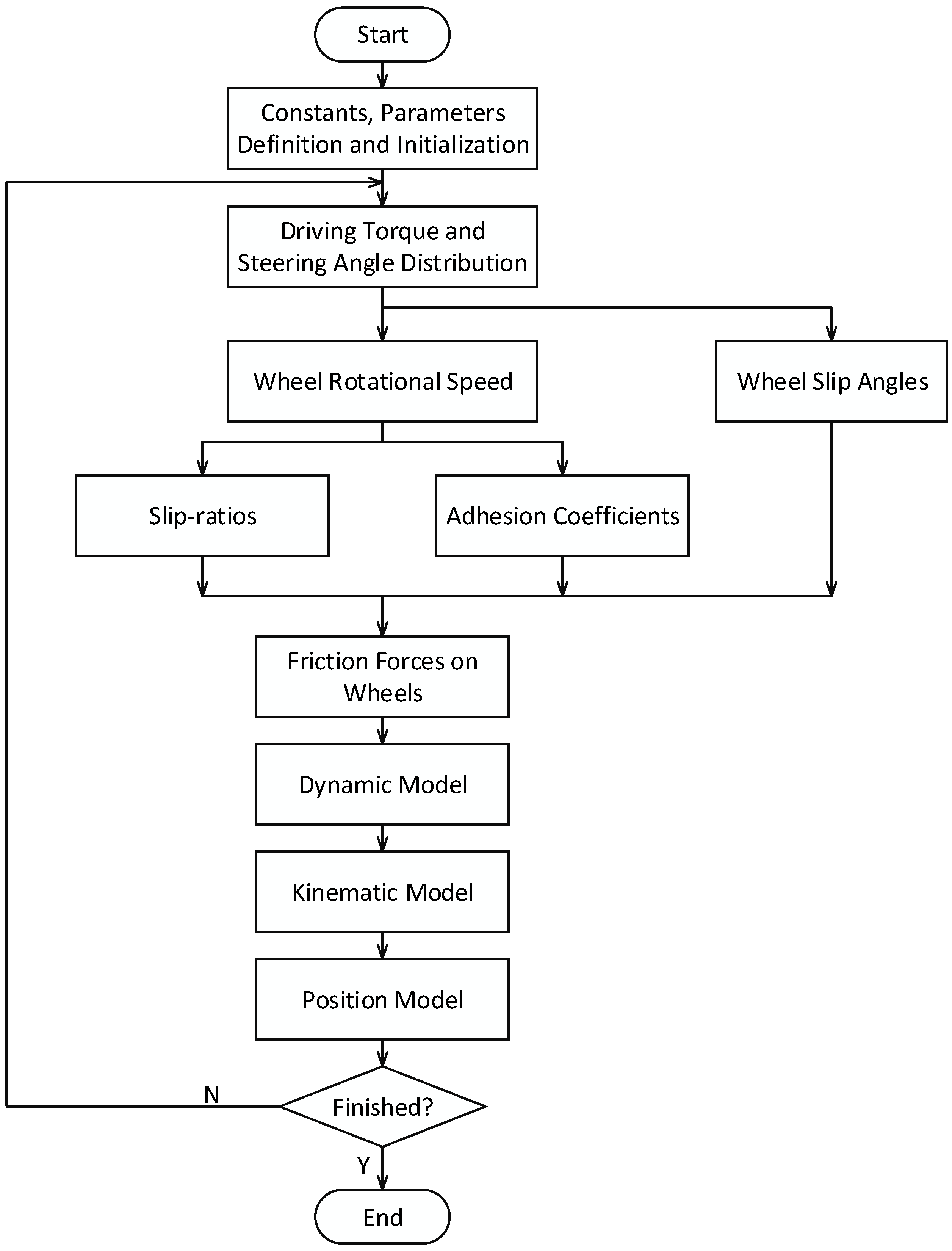
3.5. Mathematical Model Implementation Procedure

Figure 8 depicts the flowchart of the program that simulates the vehicle. Because of the limitation in computing power of the simulation hardware, all of the constants should be initialized at the beginning of the program. Additionally, in order to reduce the calculation time, lookup tables can be used for some blocks, for example, adhesion coefficients will be calculated in advance and put in a lookup table instead of repeating (5) in every sampling time. Following that, all of the models and equations are implemented with the procedure that is illustrated in the flowchart. Thereafter, this program is complied and downloaded to run on the chosen hardware platform.

Although all of the equations that contribute to the simulation model of the EV are listed in a given order and the program flowchart is also supplied, the computation procedure of the complete model should be treated carefully, as there exists several recursive calculation loops. Figure 9 presents, in detail, the running process through the equations of the EV model. The following remarks should be noted when realizing this model.

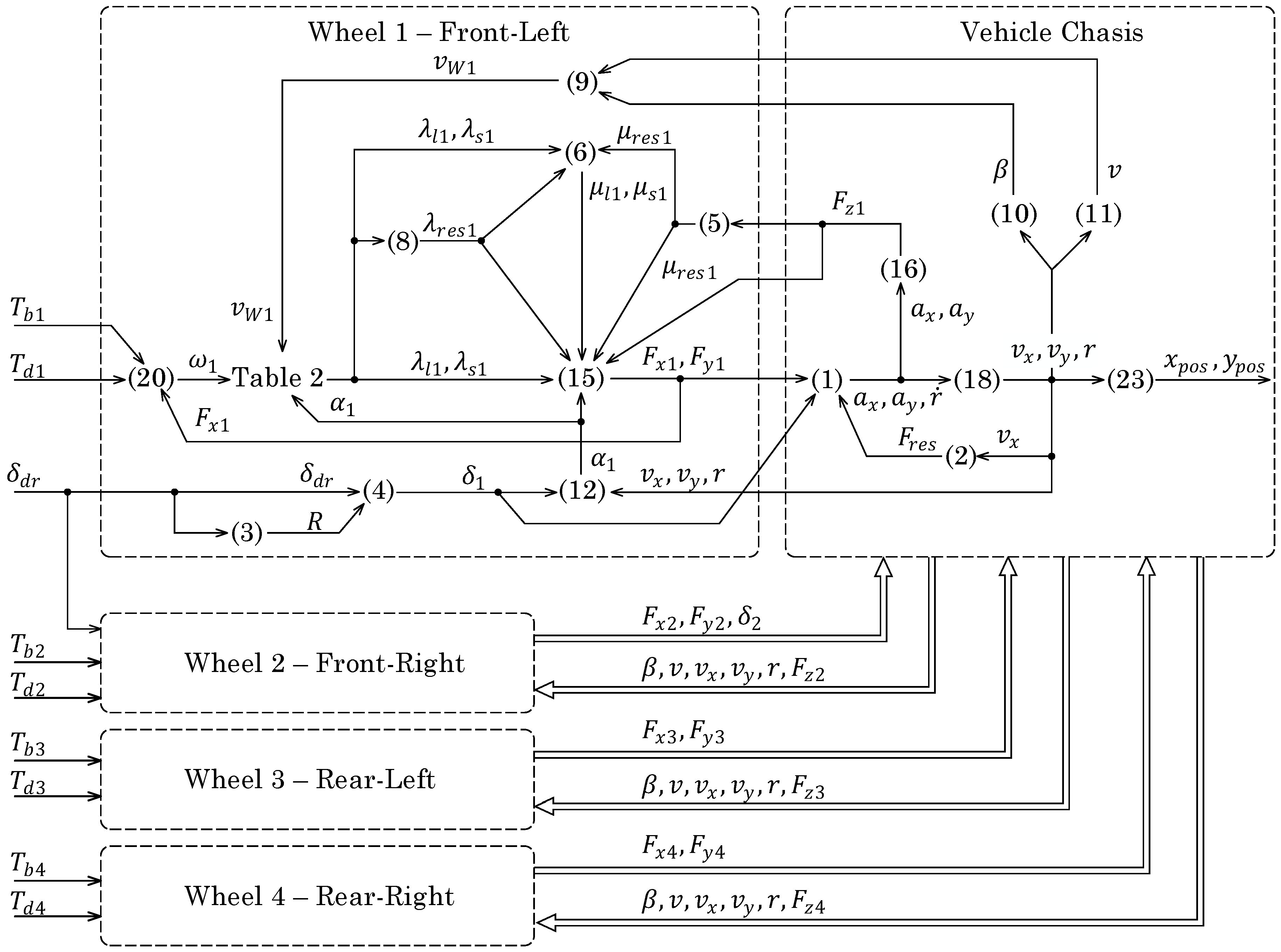
• For each equation in Figure 9, the input vectors indicate the required information for achieving the output vector, which is the result of that equation. Additionally, some equations that are the derivation of the final one may be omitted, i.e., only the most fundamental ones are shown in the flowchart.
• The calculation process is illustrated for one representative wheel, i.e., the front-left wheel, but it is identically applicable for other wheels.
• The flowchart consists of two main blocks, including the wheel model block and vehicle chassis one. The wheel block outputs the longitudinal and lateral forces, which are then incorporated with those of other wheel blocks at (1) to make the accelerations of the vehicle.
• As the front-wheel steering vehicle is mentioned as the studied object, only two steering angles at the front wheels are obtained and delivered to the vehicle chassis block. Therefore, both rear wheel blocks only generate friction forces.
• In order to avoid algebraic loop issues that are caused by the existence of recursive computation, the feedback signals, e.g., states of the vehicle, must be initialized.

In this paper, the simulation model is realized and validated on Matlab/Simulink, while using common transfer functions and S-functions to implement the system on the real-time platform without any further conversion.

4. Validation Results

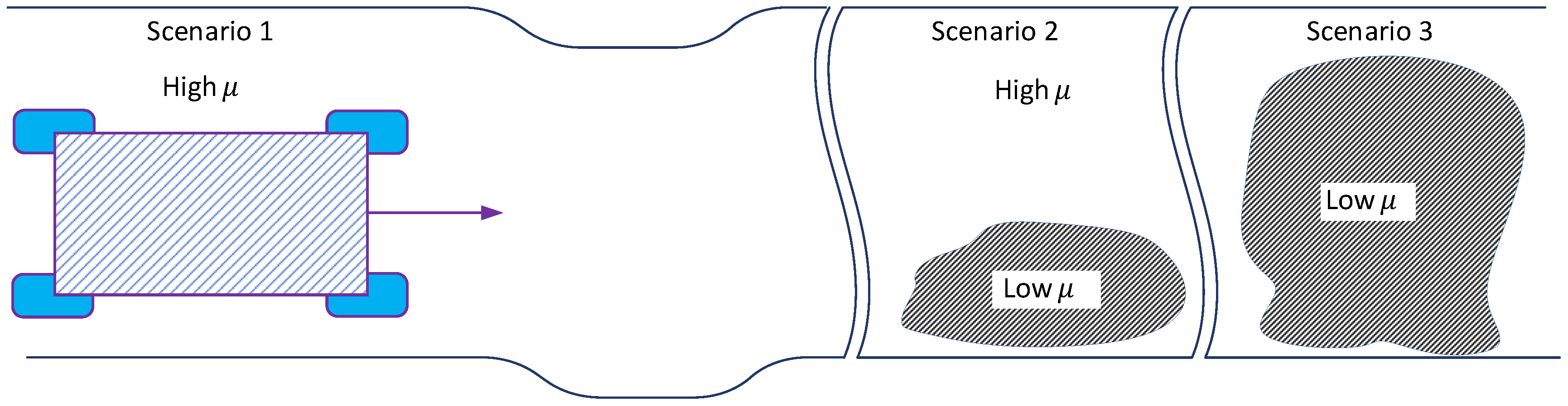
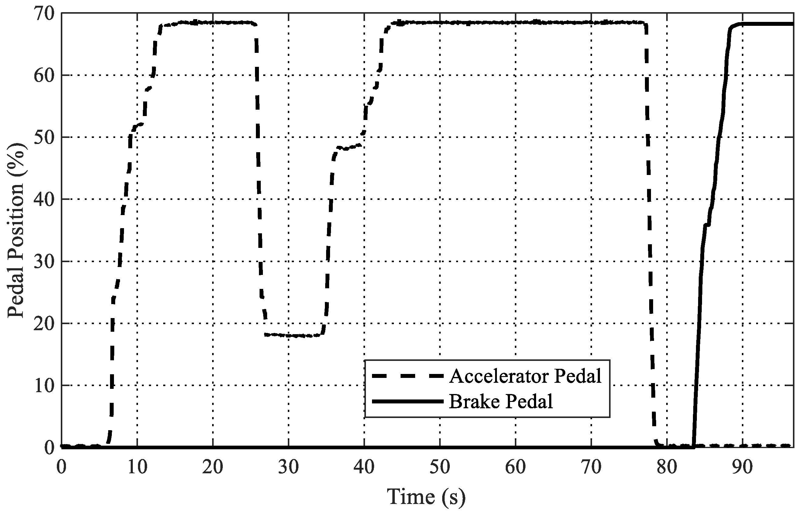
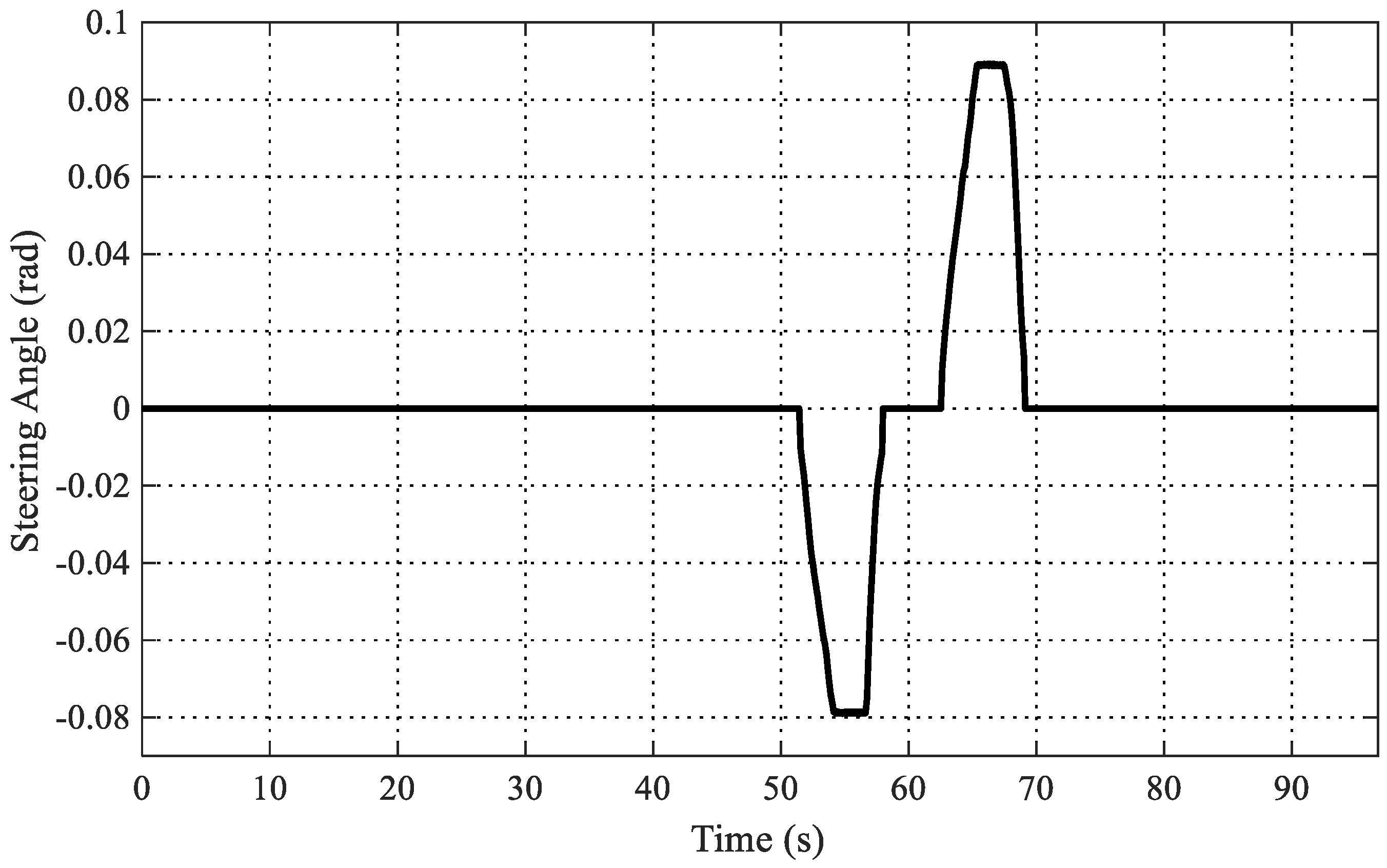
4.1. Testing Scenarios

Several representative scenarios are proposed in order to evaluate the performance of the HIL simulation system. For these tests being performed successfully, the system must be properly connected and powered. Additionally, several states or measured signals should be displayed on the screen of the host computer, which can be done by setting up in the Control Desk software. So that the driver (tester) will be able to manage the evaluation as this is the drive-able system.

In the first test case, which is also called Scenario 1, the vehicle moves on the normal road with a good adhesion coefficient $\mu$. The vehicle is accelerated by pushing the accelerator pedal. The driver can adjust the position of the pedal in order to see the change of velocity that aims to describe the longitudinal behavior of the studied vehicle. When the vehicle reaches an arbitrary speed, the driver will turn the steering wheel clockwise and then counter-clockwise continuously to show the lateral behavior of the vehicle.

Scenario 2 is carried out by letting the vehicle moving on the slippery surface with low adhesion coefficient at the right side wheels, whereas the others on the left still run on the adhesive road.

Lastly, in Scenario 3, the vehicle will be run on a poor adhesion surface that covers the whole vehicle’s track width.

The scenarios 2 and 3 both represent the typical circumstances in daily transport operation. When driving in such situations, if the control performance is poor, then the vehicle can easily loose the control and consequently the accident may happen. Figure 10 illustrates all of the proposed evaluation scenarios.

Note that there are no control algorithm applied in these test cases. Hence, in order to ensure the legal model implementation that requires reference torques for four motors at wheels, the command torque of the driver will be distributed equally. In other words, in all three scenarios, the reference torque that is supplied to each motor is one-fourth of the command torque.

$$T_{di}^{*}={\displaystyle \frac{1}{4}}{T}_{dr}$$

(24)

Additionally, the high adhesive road that is used in all the scenarios is the dry asphalt and the snow condition is adopted for low adhesive road.

The studied EV is the i-MiEV of Mitsubishi, which has the parameters listed in

Table 3. i-MiEV Parameters.

Parameters	Value	Unit
l	2550	mm
$l_f$	1199	mm
$l_r$	1351	mm
$b_f$	1475	mm
$b_r$	1475	mm
h	559	mm
$R_{eff}$	300	mm
$J_z$	900	kgm${}^2$
$J_x$	2	kgm${}^2$
$c_W$	0.29	-
A	2.49	m${}^2$
$\rho$	1.2041	kg/m${}^3$

.

4.2. Experimental Results

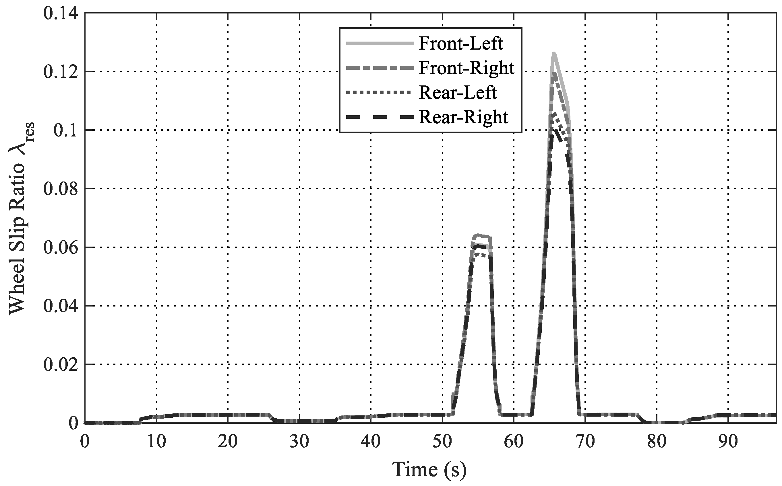
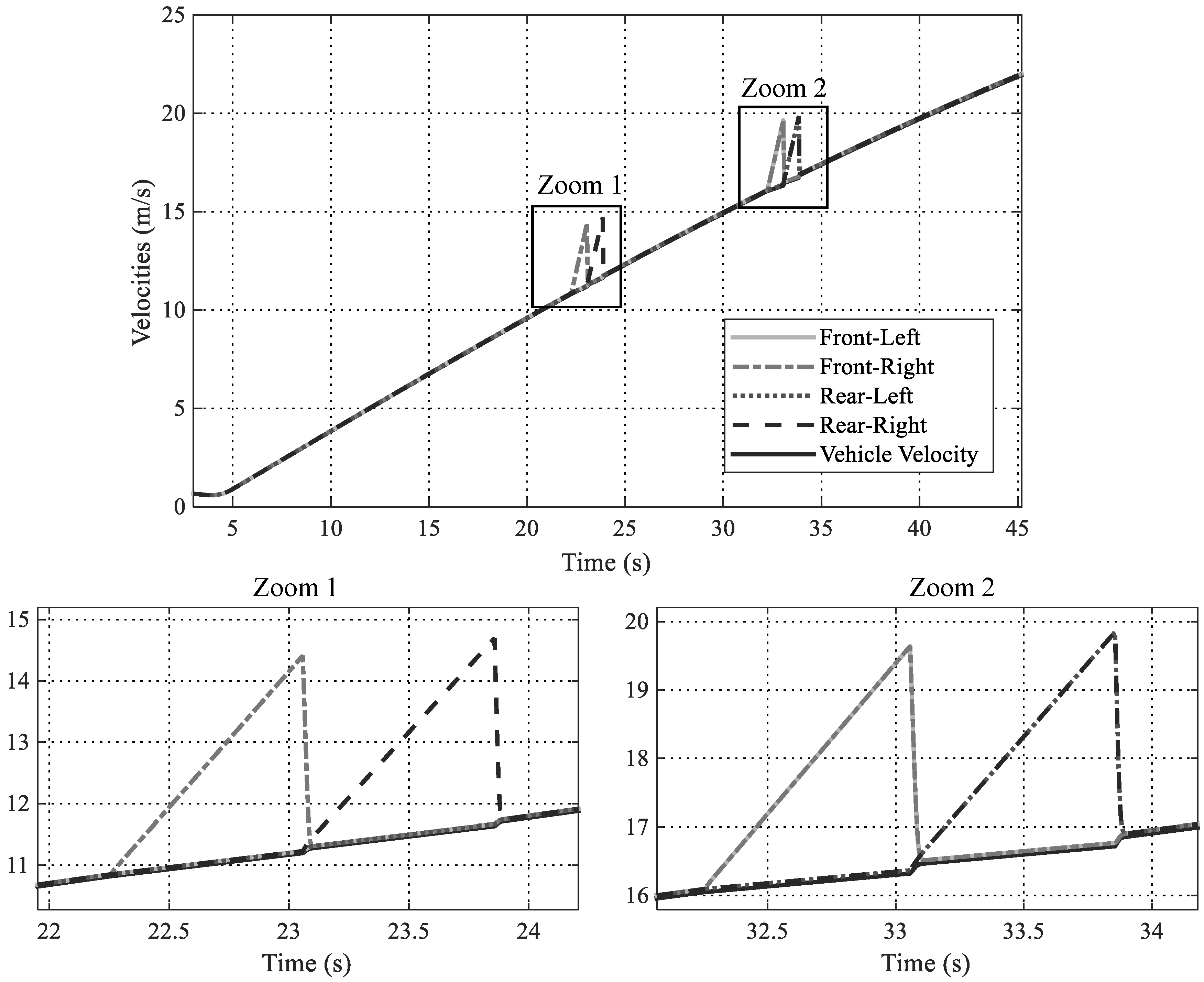
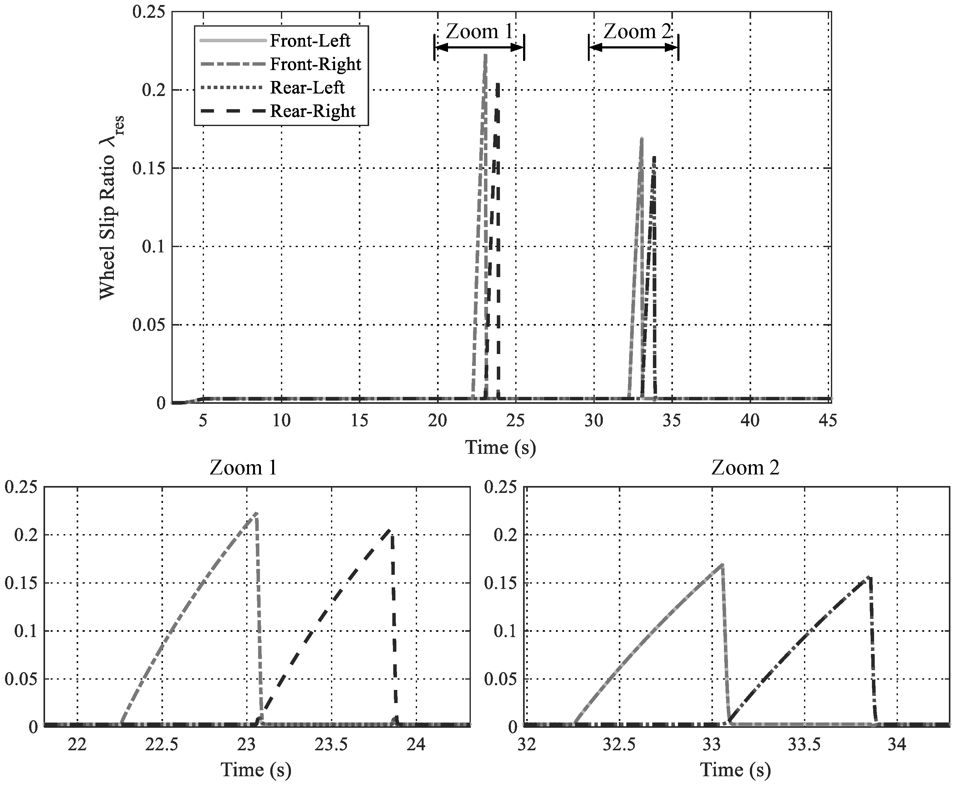
4.2.1. Scenario 1 Results

Figure 11 and Figure 12 show the driving profile that is generated by the driver for the first evaluation scenario, including accelerator, brake pedal position, and steering wheel angle, respectively. The accelerator pedal is initially pushed to 68% for about 20 s and then released to 19%. This position is kept for nearly 10 s, and then the driver increases the pressure again and holds it at 68% to t = 50 s. At this moment, the steering wheel is rotated clockwise, thus the steering angle is changed from zero to negative value. This is to imply that the car will be right cornered. After returning the wheel to zero position, the driver continues to turn left by anti-clockwise rotating the steering wheel. Until t = 70 s, the driver sets the angle to zero in order to control the car going straight. Finally, at t = 85 s, the brake pedal is pressed to slow down the vehicle.

The response of the car to the driver’s command in terms of wheel and vehicle velocities, slip-ratios at each wheel, and position are shown in Figure 13, Figure 14 and Figure 15, respectively.

In the velocity waveforms presented in Figure 13, the good quality road is reflected by the closely matching of wheel velocities and that of the vehicle. At the beginning of the test, the velocities rise following the increase of accelerator pedal position. This growing trend is flattened when the driver keeps the pedal at lower level, thus the car moves at a nearly constant speed. In the next phase of the acceleration, the vehicle reaches to around 18 m/s (65 km/h) when the accelerator pedal is kept at 68%. The velocities at wheels precisely equal to each other and also almost equal to that of the vehicle from the beginning to t = 52 s thanks to high adhesive coefficient of the road. From this moment, the driver starts cornering the vehicle which causes the differences between the velocities, as shown in two zoomed figures. The Zoom 1 shows the detailed difference at the first cornering and the Zoom 2 illustrates that of the second turning duration. At t = 78 s, the vehicle is slowed down, because the driver starts pushing the brake pedal. If the pedal is more pushed, the vehicle velocity is more decelerated, as can be seen.

Figure 14 describes the slip-ratios ${\lambda }_{res}$ of wheels, which is the remarkable feature of the proposed system. In the duration of straight movement of the vehicle, the slip-ratios are very small, due to the negligible deviation between wheel and vehicle velocities. The significant change of the slip-ratio appears when the car is being cornered. The ${\lambda }_{res}$ reaches to maximum of 0.062 in the first cornering and up to 0.123 in the second one. These values are still considered in the safe region of slip-ratio (under 0.2). However, if referring to the conventional slip-ratio calculation (7) in the previous subsection, which only takes into account the difference between wheel velocity $\omega R_{eff}$ and longitudinal velocity $v_x$, the slip-raito cannot obtain such big values. Two zoomed figures in Figure 13 are the evidences for this remark, as the difference among velocities exists, but is not noteworthy. Thanks to the aforementioned calculation presented in Table 2, the total slip-ratio is composed of longitudinal and lateral values. Hence, the significant amount of ${\lambda }_{res}$ in Figure 14 are mainly caused by lateral slip-ratio ${\lambda }_s$. In the other words, the vehicle seems to be drifted a bit when cornering at relatively high speed (18 m/s at the first time and 21 m/s at the second time).

Figure 15 illustrates the position of the vehicle on two-dimensional (2-D) plane. The trajectory acts in accordance with the driver’s command that is shown in Figure 11 and Figure 12. The car goes straight and then is turned right and left following the steering wheel reference and eventually continues straight to the end of the test. Generally, running on the good road condition, the vehicle can safely obey what the driver wants in terms of secured states of the car.

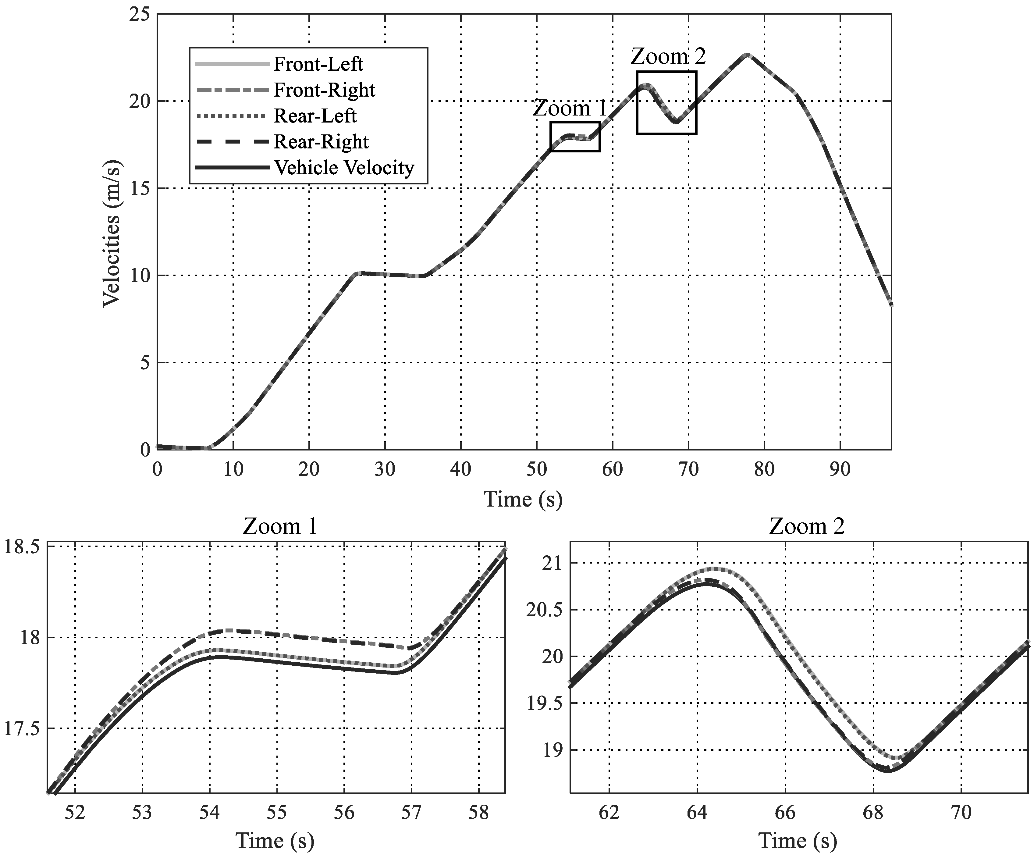
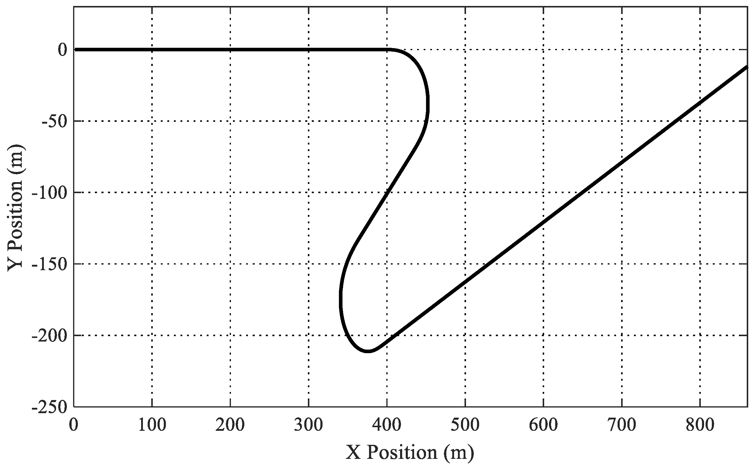
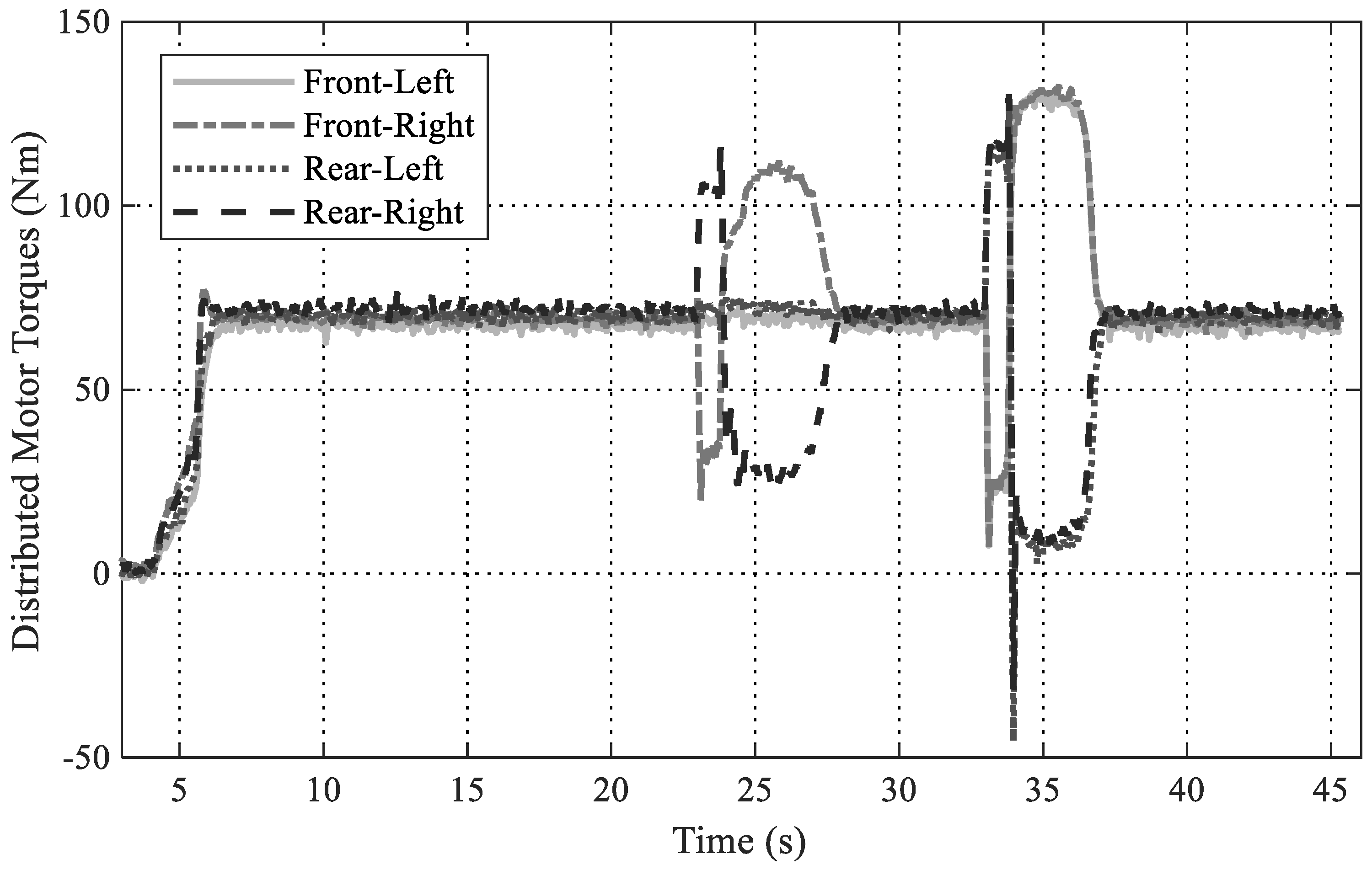
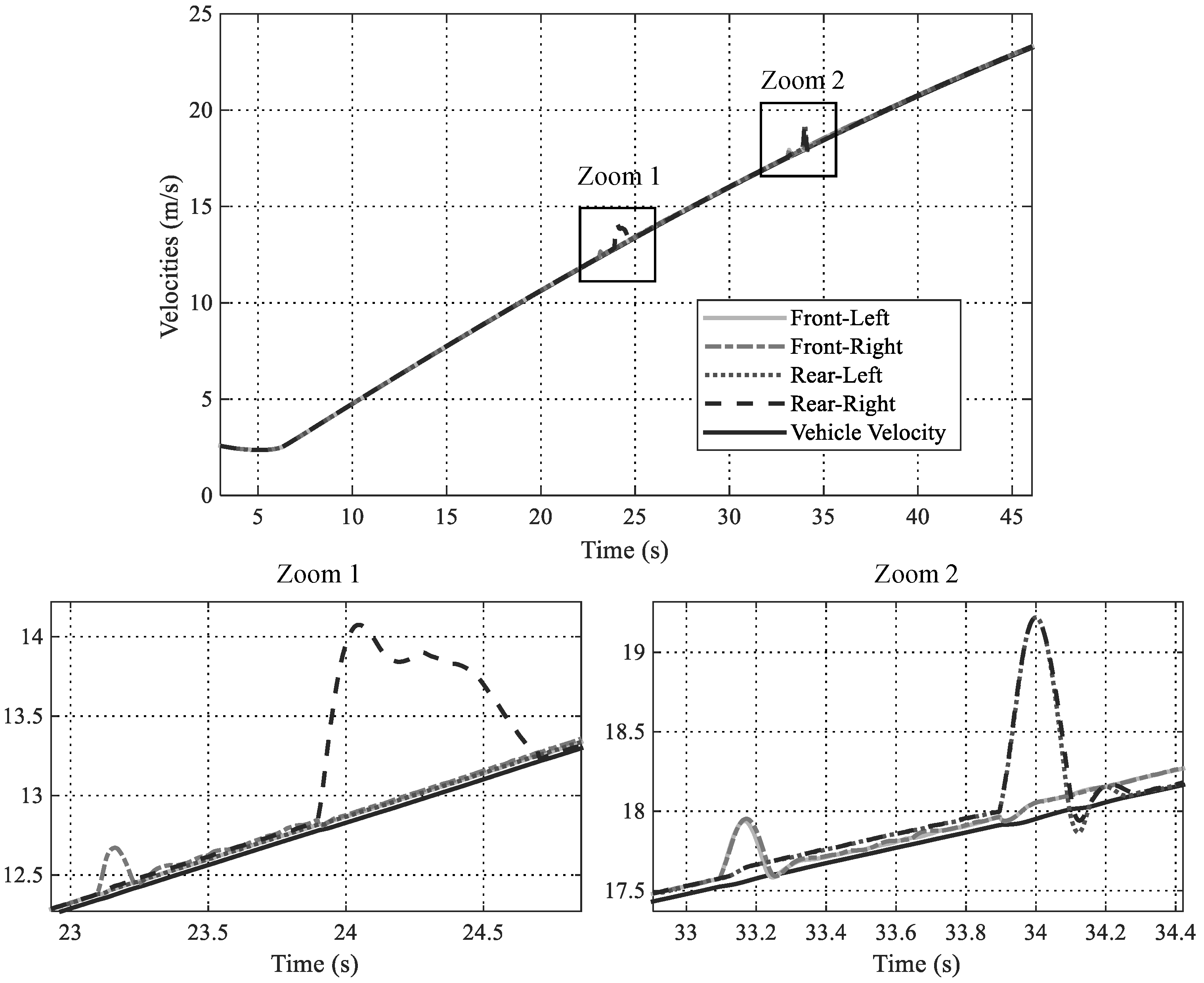
4.2.2. Scenario 2 and 3 Results

Scenarios 2 and 3 will be carried out in the same test, since they are both used for evaluation on slippery road. In these test cases, the accelerator pedal is kept constant at value of 68% while the brake one is free throughout the entire evaluation, as depicted in Figure 16. Additionally, the steering wheel is held at zero in order to imply that the car is expected going straight for the whole test.

The velocities of wheels and of the vehicle increase, obeying the given accelerator pedal position, as depicted on Figure 17. The vehicle is accelerated to about 11m/s before getting into slippery road. From this moment, evaluation scenarios are respectively started.

Scenario 2 begins at $t\approx$ 22 s; when the front-right wheel enters the low adhesive surface and, immediately, its velocity increases very fast. This wheel gets to the maximum speed of 14.3 m/s and leaves the slippery road; following that, the rear-right wheel starts running on this surface. With the same manner, its velocity also rises dramatically to approximated 14.7 m/s before returning to the good road condition. For both right wheels, after leaving the sliding surface, their velocities reduce sharply to that of other wheels and synchronously with the speed of the vehicle. On the contrary, both left wheels still work properly on the good road condition, showing by their velocity trend did not nearly change during the test. The vehicle velocity also has the same behavior to these wheels when its velocity keeps increasing all the time.

When the vehicle reaches to 16m/s of speed ($t\approx$ 32 s), once again, it gets in the sliding surface, which is Scenario 3. Different from the previous test, in this case, the two front wheels simultaneously enter the low adhesive road. The friction force is weakened, while motor torques are still remained, which results in the unexpected increase of wheel velocities. The increase in the speed of wheels only stops and reduces dramatically when they get out of the sliding surface. The same behavior happens for both rear wheels. The maximum velocity of four wheels in the test case is nearly 20 m/s. Interestingly, because there are still two wheel running on the high adhesion road while others are moving on bad condition, the vehicle velocity retained its tendency. This is the remarkable advantage of a all-wheel-driven (AWD) vehicle.

The safety aspect of the vehicle in these scenarios can be evaluated by slip-ratio, as illustrated in Figure 18. Empirically, the secured working region of the vehicle is ${\lambda }_{res}<0.2$. If the slip-ratio is larger than this number, then the vehicle will be considered to be slipping on the road, i.e., the wheel spins without adhesion on the road surface. This circumstance must be avoided, because the car may loose control easily and this is the duty of all motion controllers, e.g., Traction Control System (TCS) of Toyota or Dynamic Stability Control (DSC) of BWM. Without control, the slip-ratio of the studied vehicle gets over the value of 0.2, as depicted in the figure. Dangerously, these ratios are in the increasing tendency and, if the slippery surface is longer, then the slip-ratios will reach a much higher value. However, the behavior of the slip-ratio at wheels complies with the manner of working situation, which is the key expectation of the proposed system.

The position trajectory of the CoG of the vehicle depicted in Figure 19 also shows the serious situation, especially in the Scenario 2. The vehicle’s lateral position is changed suddenly when the side wheels come over the low $\mu$ surface. Let us focus on the instant when the front-right wheel enters the slippery surface that causes the adhesion force to be reduced at this wheel. Because the summed force of two left wheels still remains, the difference between the forces on the right and left side of the vehicle generates torque in the clockwise direction. Consequently, the vehicle rotates and moves to the right. When the front-right wheel leaves the low friction surface with high rotational speed and returns to the adhesive road, it causes a "strike force" applied to the right side. This jerks the vehicle to the left in a very small duration. This phenomenon is repeated when the rear-right wheel runs on the low adhesive road. Although the side displacement is small (under 0.5 m) and the speed of the vehicle is relatively low, this unexpected change may still cause a dangerous situation to the car and the driver. For Scenario 3, the vehicle’s trajectory is on the straight line, because there is no lateral force or different friction forces between the left and right sides of the vehicle.

5. Application Example Using the Proposed HIL Simulation System

5.1. Control System Configuration

An application example of control system based on optimal driving force distribution algorithm [40] has been implemented in order to further validate the performance of the HIL simulation system. This research work exploits the “glocal” (global-local) control scheme, in which the global controller is responsible for generating distributed reference driving forces $F_{xi}^{*}$ to guarantee the coordination among the motions of wheels and of the vehicle, the local controllers create reference motor torques $T_{di}^{*}$ that are based on the generated force commands in order to ensure the secured slip-ratios at the wheels of the vehicle. Figure 20 shows the configuration of the example control system.

The input of the control system is the driving force $F_{dr}$, i.e., driver’s command; thus, the accelerator pedal signal should be redefined instead of aforementioned $T_{dr}$. As mentioned about the design procedure earlier, the whole control system of this application will be deployed on the eZdsp F28335 Control Card. In Figure 20, one local controller for the front-left wheel is described. Other controllers for other wheels are designed identically. The reference motor torques that are generated from the control algorithm are multiplexed and transmitted to the vehicle through the CAN bus. Whereas, the measured signals, including wheel rotational speeds and longitudinal acceleration of the car, are connected to ADC ports of the control card, as they are analogous. On the vehicle model side, instead of using sensors as real experiments do, such signals can be output from DAC ports of the DS1103 Controller Board, which is one of the advantages of the proposed HIL simulation system.

The detail distribution algorithm and control design can be found in [40]. For the driving force observer as well as the slip-ratio estimator, one can find them in [41], as the development of motion controller is not in the scope of this paper.

In this section, the example control scheme will be validated only with Scenarios 2 and 3, because these test cases can effectively highlight the dominant features of the algorithm.

5.2. Results

Figure 21, Figure 22, Figure 23 and Figure 24 illustrated the validation results of the example control system running on the proposed HIL simulation system.

Let us focus on the reference motor torque that is shown in Figure 21. From the driving force command, four torque values are generated, which are quite stable at the beginning of the test. However, taking a closer look to the waveform within this duration, the controller distributes more torque to the rear wheels than to the front ones. This actually makes sense, because, referring to (16), the normal force at rear wheels increase when accelerating. Hence, more wheel torque can exploit more friction force, leading to better acceleration, which also can be seen in Figure 22 for longitudinal friction force.

When $t\approx$ 23 s, Scenario 2 is carried out, which leads to the small difference between in velocity of the right-front wheel and the vehicle, as shown in the Zoom 1 of Figure 23. Remarkably, when traveling on the low $\mu$ condition, the friction force decreases sharply, the control system immediately reduces motor torque of the respective wheel, i.e., the right-front one in this case, in order to keep the slip-ratio at a properly small value, as shown in Figure 24. Simultaneously, the torque at the rear-right wheel is increased in order to compensate the reduction in friction force of the sliding wheel. Consequently, the car is kept going safely in a secured state. The same control behavior is applied within the remained Scenario 2 duration, in which the front-right wheel torque is boosted to pull the right side of the vehicle when the rear-right one is running on low friction surface.

Scenario 3 is taken part in the test when $t\approx$ 33 s. When both front wheels are traveling on the sliding road, the motor torques are decreased, following the reduction of the friction forces and, thus, keeping the slip-ratio at a small value (around 0.02, as depicted in the Zoom 2 of the Figure 24). The controller compensates for the loss in the total driving force by reinforcing torque at both rear wheels. This leads to the sum of all longitudinal forces remaining the reference value. The same response is made by the controller when the rear wheels are running on the low adhesive surface as the final section of Scenario 3.

For the whole validation, Figure 24 shows the advantage of the control scheme in the safety aspect, in which the slip-ratios are kept under the maximum value of about 0.09, much smaller than those of uncontrolled schema results. Moreover, the wheel speed is controlled very fast; therefore, the unexpected sliding duration is significantly small and the vehicle can overcome the bad road condition smoothly.

6. Conclusions

In this paper, an experimental platform that is based on signal HIL simulation system for 4-IWM EVs has been proposed. The HIL system is derived from detailed dynamic models in longitudinal, lateral, and yaw directions, which are frequently used in motion control of EVs. The term “detailed” is shown in adhesion coefficients calculation, slip-ratio computation, and tire force models, which are further complex than the conventional ones. Thanks to these features, the specific aspects in behavior of the vehicle is emphasized and allow for better control performance assessment. The advantages of the proposed signal HIL simulation system are illustrated through various evaluation plans with several road conditions and different driving scenarios. The capability and application of the HIL system are also confirmed by examining a representative control strategy in optimal driving force distribution for four wheels of the studied vehicle. Being developed from DS1103 and F28335 digital signal controllers that are very common research platforms, the proposed system is cost-effective, safe, open, and can be used widely.

In the future, this work on signal HIL simulation system can be extended in both directions: (i) applying this system to other vehicle control problems and (ii) expanding the system model. Autonomous driving is an example of the former direction, in which adaptive cruise control or automatic lane-changing can exploit the position model of this HIL platform. On the other hand, the proposed system can be enlarged by adding models of energy storage devices or specific electric motors. By that, the system can be used for research on energy management and electric drives that illustrate the open and expandable features of the proposed experimental platform.

References

1. Weiss, M.; Cloos, K.C.; Helmers, E. Energy efficiency trade-offs in small to large electric vehicles. Environ. Sci. Eur. 2020, 32. [Google Scholar] [CrossRef] [Green Version]
2. Helmers, E.; Marx, P. Electric cars: Technical characteristics and environmental impacts. Environ. Sci. Eur. 2012, 24, 1–15. [Google Scholar] [CrossRef] [Green Version]
3. Karki, A.; Phuyal, S.; Tuladhar, D.; Basnet, S.; Shrestha, B.P. Status of Pure Electric Vehicle Power Train Technology and Future Prospects. Appl. Syst. Innov. 2020, 3, 35. [Google Scholar] [CrossRef]
4. Yamamoto, M.; Kakisaka, T.; Imaoka, J. Technical trend of power electronics systems for automotive applications. Jpn. J. Appl. Phys. 2020, 59. [Google Scholar] [CrossRef]
5. Chau, K.T. Electric Vehicle Machine and Drives—Design, Analysis and Application; John Wiley & Sons: Singapore, 2015. [Google Scholar]
6. Hori, Y. Motion control of electric vehicles and prospects of supercapacitors. IEEJ Trans. Electr. Electron. Eng. 2009, 4, 231–239. [Google Scholar] [CrossRef]
7. Hussain, S.; Ahmed, M.A.; Kim, Y.C. Efficient Power Management Algorithm Based on Fuzzy Logic Inference for Electric Vehicles Parking Lot. IEEE Access 2019, 7, 65467–65485. [Google Scholar] [CrossRef]
8. Balaska, H.; Ladaci, S.; Schulte, H.; Djouambi, A. Adaptive cruise control system for an electric vehicle using a fractional order model reference adaptive strategy. IFAC-PapersOnLine 2019, 52, 194–199. [Google Scholar] [CrossRef]
9. Ivanov, V.; Savitski, D.; Shyrokau, B. A Survey of Traction Control and Antilock Braking Systems of Full Electric Vehicles with Individually Controlled Electric Motors. IEEE Trans. Veh. Technol. 2015, 64, 3878–3896. [Google Scholar] [CrossRef]
10. He, H.; Peng, J.; Xiong, R.; Fan, H. An acceleration slip regulation strategy for four-wheel drive electric vehicles based on sliding mode control. Energies 2014, 7, 3748–3763. [Google Scholar] [CrossRef] [Green Version]
11. Lin, C.; Xu, Z. Wheel torque distribution of four-wheel-drive electric vehicles based on multi-objective optimization. Energies 2015, 8, 3815–3831. [Google Scholar] [CrossRef] [Green Version]
12. Tian, J.; Tong, J.; Luo, S. Differential Steering Control of Four-Wheel Independent-Drive Electric Vehicles. Energies 2018, 11, 2892. [Google Scholar] [CrossRef] [Green Version]
13. Park, J.; Jang, I.G.; Hwang, S.H. Torque distribution algorithm for an independently driven electric vehicle using a fuzzy control method: Driving stability and efficiency. Energies 2018, 11, 3479. [Google Scholar] [CrossRef] [Green Version]
14. Thanh, V.D.; Ta, C.M. A Universal Dynamic and Kinematic Model of Vehicles. In Proceedings of the 2015 IEEE Vehicle Power and Propulsion Conference (VPPC), Montreal, QC, Canada, 19–22 October 2015; pp. 1–6. [Google Scholar] [CrossRef]
15. Baek, S.Y.; Kim, Y.S.; Kim, W.S.; Baek, S.M.; Kim, Y.J. Development and Verification of a Simulation Model for 120 kW Class Electric AWD (All-Wheel-Drive) Tractor during Driving Operation. Energies 2020, 3, 2422. [Google Scholar] [CrossRef]
16. Pappalardo, C.M.; Lombardi, N.; Guida, D. A model-based system engineering approach for the virtual prototyping of an electric vehicle of class l7. Eng. Lett. 2020, 28, 215–234. [Google Scholar]
17. Mechanical Simulation. Introduction to CarSim. Available online: https://www.carsim.com/downloads/pdf/ (accessed on 31 October 2020).
18. TESIS-DYNAware. veDYNA Entry—The Perfect Entry Point to Vehicle Dynamics Simulation. Available online: https://www.tesis-dynaware.com/ (accessed on 31 October 2020).
19. Bouscayrol, A. Hardware-in-the-loop simulation. In Industrial Electronics Handbook, 2nd ed.; Taylor and Francis: Chicago, IL, USA, 2011; Chapter M35. [Google Scholar]
20. Messier, P.; Nguyễn, B.H.; LeBel, F.A.; Trovão, J.P.F. Disturbance observer-based state-of-charge estimation for Li-ion battery used in light electric vehicles. J. Energy Storage 2020, 27, 101144. [Google Scholar] [CrossRef]
21. Kermani, S.; Trigui, R.; Delprat, S.; Jeanneret, B.; Guerra, T.M. PHIL implementation of energy management optimization for a parallel HEV on a predefined route. IEEE Trans. Veh. Technol. 2011, 60, 782–792. [Google Scholar] [CrossRef]
22. Nguyen, B.H.; German, R.; Trovao, J.P.F.; Bouscayrol, A. Real-time energy management of battery/supercapacitor electric vehicles based on an adaptation of pontryagin’s minimum principle. IEEE Trans. Veh. Technol. 2019, 68, 203–212. [Google Scholar] [CrossRef] [Green Version]
23. Mayet, C.; Delarue, P.; Bouscayrol, A.; Chattot, E. Hardware-In-the-Loop Simulation of Traction Power Supply for Power Flows Analysis of Multitrain Subway Lines. IEEE Trans. Veh. Technol. 2017, 66, 5564–5571. [Google Scholar] [CrossRef]
24. Yuan, Y.; Zhang, J.; Li, Y.; Li, C. A Novel Regenerative Electrohydraulic Brake System: Development and Hardware-in-Loop Tests. IEEE Trans. Veh. Technol. 2018, 67, 11440–11452. [Google Scholar] [CrossRef]
25. Zhang, H.; Zhang, Y.; Yin, C. Hardware-in-the-Loop Simulation of Robust Mode Transition Control for a Series-Parallel Hybrid Electric Vehicle. IEEE Trans. Veh. Technol. 2016, 65, 1059–1069. [Google Scholar] [CrossRef]
26. Reitinger, J.; Balda, P.; Schlegel, M. Steam turbine hardware in the loop simulation. In Proceedings of the 2017 21st International Conference on Process Control, PC 2017, Štrbské Pleso, Slovakia, 6–9 June 2017; pp. 380–385. [Google Scholar] [CrossRef]
27. Yang, J.; Konno, A.; Abiko, S.; Uchiyama, M. Hardware-in-the-loop simulation of massive-payload manipulation on orbit. Robomech J. 2018, 5. [Google Scholar] [CrossRef]
28. Wu, J.; Cheng, Y.; Srivastava, A.K.; Schulz, N.N.; Ginn, H.L. Hardware in the Loop test for power system modeling and simulation. In Proceedings of the 2006 IEEE PES Power Systems Conference and Exposition, PSCE 2006, Atlanta, GA, USA, 29 October–1 November 2006; pp. 1892–1897. [Google Scholar] [CrossRef]
29. Magalhães, Z.; Murilo, A.; Lopes, R.V. Development and evaluation with MIL and HIL simulations of a LQR-based upper-level electronic stability control. J. Braz. Soc. Mech. Sci. Eng. 2019, 41, 327. [Google Scholar] [CrossRef]
30. Vo-Duy, T.; Ta, M.C. A signal hardware-in-the-loop model for electric vehicles. Robomech J. 2016, 3, 29. [Google Scholar] [CrossRef] [Green Version]
31. Nie, P.; Wu, Y.; Liang, X. Design of HIL Test System for VCU of Pure Electric Vehicle. In Proceedings of the 2017 2nd International Conference on Materials Science, Machinery and Energy Engineering (MSMEE 2017), Dalian, China, 13–14 May 2017; Volume 123, pp. 867–871. [Google Scholar] [CrossRef] [Green Version]
32. Xia, J.L.; Diao, Q.; Sun, W.; Xing, Z.; Yuan, X.; Dong, T. Development of low cost hardware-in-the-loop test system and a case study for electric vehicle controller. In Proceedings of the 2016 International Conference on Applied System Innovation, (ICASI), Okinawa, Japan, 26–30 May 2016; pp. 4–7. [Google Scholar] [CrossRef]
33. Ramaswamy, D.; McGee, R.; Sivashankar, S.; Deshpande, A.; Allen, J.; Rzemien, K.; Stuart, W. A Case Study in Hardware-In-The-Loop Testing: Development of An ECU for a Hybrid Electric Vehicle; SAE Technical Papers; SAE International: Warrendale, PA, USA, 2004. [Google Scholar] [CrossRef]
34. Yan, Y.; Liu, C.; Ma, X.; Zhang, Y. Hardware-in-loop real-time simulation of electrical vehicle using multi-simulation platform based on data fusion approach. Int. J. Distrib. Sens. Netw. 2019, 15. [Google Scholar] [CrossRef]
35. Nam, K.H. AC Motor Control and Electrical Vehicle Applications, 2nd ed.; Taylor & Francis: Boca Raton, FL, USA, 2019. [Google Scholar]
36. Kiencke, U.; Nielsen, L. Automotive Control System; Springer: Berlin/Heidelberg, Germany, 2005. [Google Scholar]
37. Pacejka, H.B. Tire and Vehicle Dynamics, 3rd ed.; Butterworth-Heinemann: Oxford, UK, 2012. [Google Scholar]
38. Rajamani, R. Vehicle Dynamics and Control, 2nd ed.; Springer: New York, NY, USA, 2012. [Google Scholar]
39. Jazar, R.N. Vehicle Dynamics: Theory and Application; Springer: New York, NY, USA, 2009. [Google Scholar]
40. Wang, Y.; Fujimoto, H.; Hara, S. Driving Force Distribution and Control for EV With Four In-Wheel Motors: A Case Study of Acceleration on Split-Friction Surfaces. IEEE Trans. Ind. Electron. 2017, 64, 3380–3388. [Google Scholar] [CrossRef]
41. Maeda, K.; Fujimoto, H.; Hori, Y. Four-wheel driving-force distribution method based on driving stiffness and slip ratio estimation for electric vehicle with in-wheel motors. In Proceedings of the 2012 IEEE Vehicle Power and Propulsion Conference, VPPC 2012, Seoul, Korea, 9–12 October 2012; pp. 1286–1291. [Google Scholar] [CrossRef]
Figure 1. System Configuration for Simulation.
Energies 13 06448 g001
Figure 2. Configuration of the proposed Hardware-in-the-loop simulation system.
Energies 13 06448 g002
Figure 3. The Complete Hardware-in-the-loop Simulation System.
Energies 13 06448 g003
Figure 4. Forces Applied on the Vehicle.
Energies 13 06448 g004
Figure 5. Different μ λ characteristics by Burckhardt tire-road model.
Energies 13 06448 g005
Figure 6. Friction forces acting on a wheel. F l and F s are aligned with the actual movement direction of the wheel which is indicated by the vector v W . Vector F r e s is the sum of F l and F s . The longitudinal and side forces F x and F y can be achieved by the projection of F r e s on the ( O x y ) W , which is in association with the wheel coordinate.
Energies 13 06448 g006
Figure 7. Position of the vehicle in two-dimension earth-fixed coordinate. The velocities v x and v y are associated with vehicle body-fixed frame. Sum of the projections of these vectors on the earth-fixed coordinate ( O x y ) e are v x t r a n s and v y t r a n s , which are then used for the position model of the vehicle.
Energies 13 06448 g007
Figure 8. Program Flowchart for the Signal Hardware-In-the-Loop (HIL) Simulation System.
Energies 13 06448 g008
Figure 9. Calculation flow for 4-wheel-driven EV simulation model. For simplification, the representative wheel 1 is shown. The calculation procedure for other wheels is identically the same.
Energies 13 06448 g009
Figure 10. Scenarios for HIL Simulation System Evaluation.
Energies 13 06448 g010
Figure 11. Accelerator and Brake Pedal Position for Scenario 1.
Energies 13 06448 g011
Figure 12. Steering Wheel Angle for Scenario 1.
Energies 13 06448 g012
Figure 13. Velocities of Wheels and Vehicle for Scenario 1.
Energies 13 06448 g013
Figure 14. Slip-ratio at Wheels for Scenario 1.
Energies 13 06448 g014
Figure 15. Position of the Vehicle for Scenario 1.
Energies 13 06448 g015
Figure 16. Accelerator and Brake Pedal Position for Scenario 2 and 3.
Energies 13 06448 g016
Figure 17. Velocity of Wheels and Vehicle for Scenario 2 and 3. The Zoom 1 is associated with Scenario 2 and the Zoom 2 is for Scenario 3.
Energies 13 06448 g017
Figure 18. Slip-ratio at Wheels for Scenario 2 and 3. The Zoom 1 is associated with Scenario 2 and the Zoom 2 is for Scenario 3.
Energies 13 06448 g018
Figure 19. Position of the Vehicle for Scenario 2 and 3.
Energies 13 06448 g019
Figure 20. Configuration of Driving Force Distribution and Control for EV with Four In-Wheel Motors, adapted with implementation on the proposed HIL simulation system.
Energies 13 06448 g020
Figure 21. Distributed Motor Torque Generated by the Control System.
Energies 13 06448 g021
Figure 22. Longitudinal Driving Forces Acted on each Wheels.
Energies 13 06448 g022
Figure 23. Wheel and Vehicle Velocities. The Zoom 1 is associated with Scenario 2 and the Zoom 2 is for Scenario 3.
Energies 13 06448 g023
Figure 24. Slip-ratio at each Wheels. The Zoom 1 is associated with Scenario 2 and the Zoom 2 is for Scenario 3.
Energies 13 06448 g024