Predicting the Surveillance Data in a Low-Permeability Carbonate Reservoir with the Machine-Learning Tree Boosting Method and the Time-Segmented Feature Extraction

Abstract

Predictive analysis of the reservoir surveillance data is crucial for the high-efficiency management of oil and gas reservoirs. Here we introduce a new approach to reservoir surveillance that uses the machine learning tree boosting method to forecast production data. In this method, the prediction target is the decline rate of oil production at a given time for one well in the low-permeability carbonate reservoir. The input data to train the model includes reservoir production data (e.g., oil rate, water cut, gas oil ratio (GOR)) and reservoir operation data (e.g., history of choke size and shut-down activity) of 91 producers in this reservoir for the last 20 years. The tree boosting algorithm aims to quantitatively uncover the complicated hidden patterns between the target prediction parameter and other monitored data of a high variety, through state-of-the-art automatic classification and multiple linear regression algorithms. We also introduce a segmentation technique that divides the multivariate time-series production and operation data into a sequence of discrete segments. This feature extraction technique can transfer key features, based on expert knowledge derived from the in-reservoir surveillance, into a data form that is suitable for the machine learning algorithm. Compared with traditional methods, the approach proposed in this article can handle surveillance data in a multivariate time-series form with different strengths of internal correlation. It also provides capabilities for data obtained in multiple wells, measured from multiple sources, as well as of multiple attributes. Our application results indicate that this approach is quite promising in capturing the complicated patterns between the target variable and several other explanatory variables, and thus in predicting the daily oil production rate.

1. Introduction

In recent years, the oil and gas industry began to be aware that the collection of large amounts of data coming from both gauges and specific events allows engineers, by applying artificial intelligence algorithms, to better manage the fields and reduce the maintenance cost. For example, predictive analysis of the reservoir surveillance data (e.g., production rate, following pressure) can help to identify in advance some possible failure of equipment and to intervene before an event occurs [1].

The basic idea of machine learning is to develop algorithms to parse data, learn from them, and then make decisions and predictions about real-world events. Unlike traditional physics-driven software for specific tasks, machine learning uses a large amount of data to “train” and “learn” how to accomplish tasks through the general data-driven approach. Machine learning comes directly from the early field of artificial intelligence. Traditional algorithms include decision tree, clustering, Bayesian classification, support vector machine, expectation–maximization algorithm (EM), Adaboost, and so on [2,3]. In terms of learning methods, machine learning algorithms can be divided into supervised learning (such as classification problems), unsupervised learning (such as clustering problems), semi-supervised learning, ensemble learning, in-depth learning, and reinforcement learning. Traditional machine learning algorithms in fingerprint recognition, object detection, and other fields basically meet the requirements of commercialization, but each case is challenging to be further improved until the emergence of deep learning algorithms. The deep learning algorithms can be roughly understood as a neural network structure with multiple hidden layers. In order to improve the training effect of the neural network, people have made corresponding adjustments to the connection method and activation function of neurons [4,5,6].

It is reported that hundreds of application scenarios in petroleum upstream can be optimized by the machine learning technology, scoping from oil/gas exploration, drilling, production and reservoir management [7,8]. For example, Poulton reported applying the artificial neural network (ANN) to extract structural lineaments and lithological information from the seismic data [9]. Alizadeh et al. applied the artificial neural networks (ANN) correlating sonic/porosity logs and the total organic carbon (TOC), which could reduce uncertainty and costs in the oil and gas exploration and exploitation [10]. Ross improved the resolution and clarity of seismic data in the Permian Basin by unsupervised learning. Moran used ANNs to predict the rate of penetration and so better estimate the drill time [11]. Arabloo et al. applies the support vector machine algorithm to estimate oxygen-steam ratios in coal gasification process. The average absolute error between their modeling outputs and real data is reported lower than 1.0% [12]. Sidaoui predicted the optimum injection rate of carbonate acidizing [13]. Kamari et al. evaluates the performance and applicability of various artificial lift methods by the least square support vector machine, using the tubing size and designed oil rate as input [14]. Chamkalani et al. introduced the least square support vector machine (LSSVM) to predict the asphaltene deposition. The particle swarm optimization technique is employed to optimize the key parameters, and an R2 is achieved for the testing phase [15]. Rashidi and Asadi used ANNs to predict formation pore pressure from the drilling data [16]. Dzurman et al. proposed the data-driven modeling approach to quantitatively rank and assess reservoirs of high heterogeneities, using numerical flow simulation result to construct a training data set consisting various scenarios [17]. Chang and Zhang identified the processes of the fluid flow in formations via combined data-driven and data-assimilation methods [18]. Zendehbouhi et al. reviewed the applications of hybrid black-box models in chemical, petroleum and energy systems [19]. Wang discussed the robust numerical handling of hydraulic fractures in tight reservoirs with the physics-based modeling approach, and suggested extending this method with machine learning for further analysis [20,21,22,23]. The literature above mainly focuses on the application of machine learning in geological interpretation, characterization, and drilling optimizations. A few state-of-the-art studies are published in recent years on the reservoir surveillance analysis and prediction. Chang et al. apply the machine learning in transient surveillance in a deep-water oil field [24]. Pan et al. utilize a physics-based approach to denoise the outliers and generate missing production history for a Cascated long short-term memory network for unconventional reservoirs [25]. These methods can handle huge amounts of dynamic data and have achieved certain success in field applications. Al-Fattah applied the neural network approach to predict the U.S. natural gas production. This model can be used to quantitatively examine the various physical and economic factors of future gas production [26]. However, to the best of our knowledge, it is challenging to incorporate multiple attributes with these machine learning frameworks. Most reservoir surveillance data based on our experiences is in multivariate time-series form with different strengths of internal correlation. The capacity to utilize as much informative data as possible is essential for a powerful machine learning algorithm.

In this paper, we introduce our novel machine learning-based predictive analysis of the production data, which is able to extract useful information of multiple dynamic attributes from multiple wells. More specifically, our goal is to develop an approach to predict the produced oil rate for an individual well in the next few months. Our research is conducted based on the reservoir surveillance data of a real-case carbonate reservoir with about 91 producers for the last 20 years. To motivate our approach and give readers some intuition of the problem, we first present some associated challenges and discuss the drawback of current practices for such a problem.

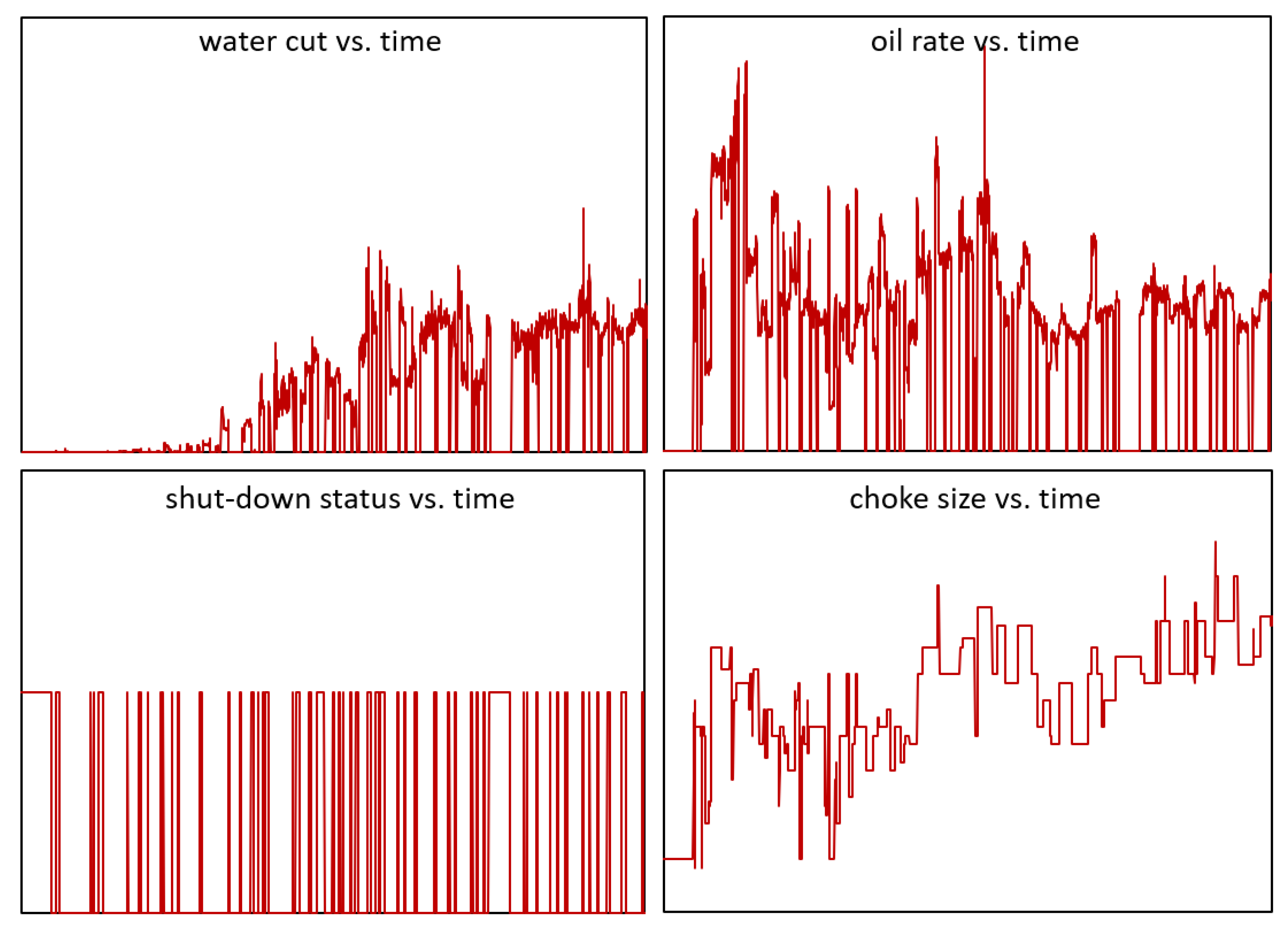
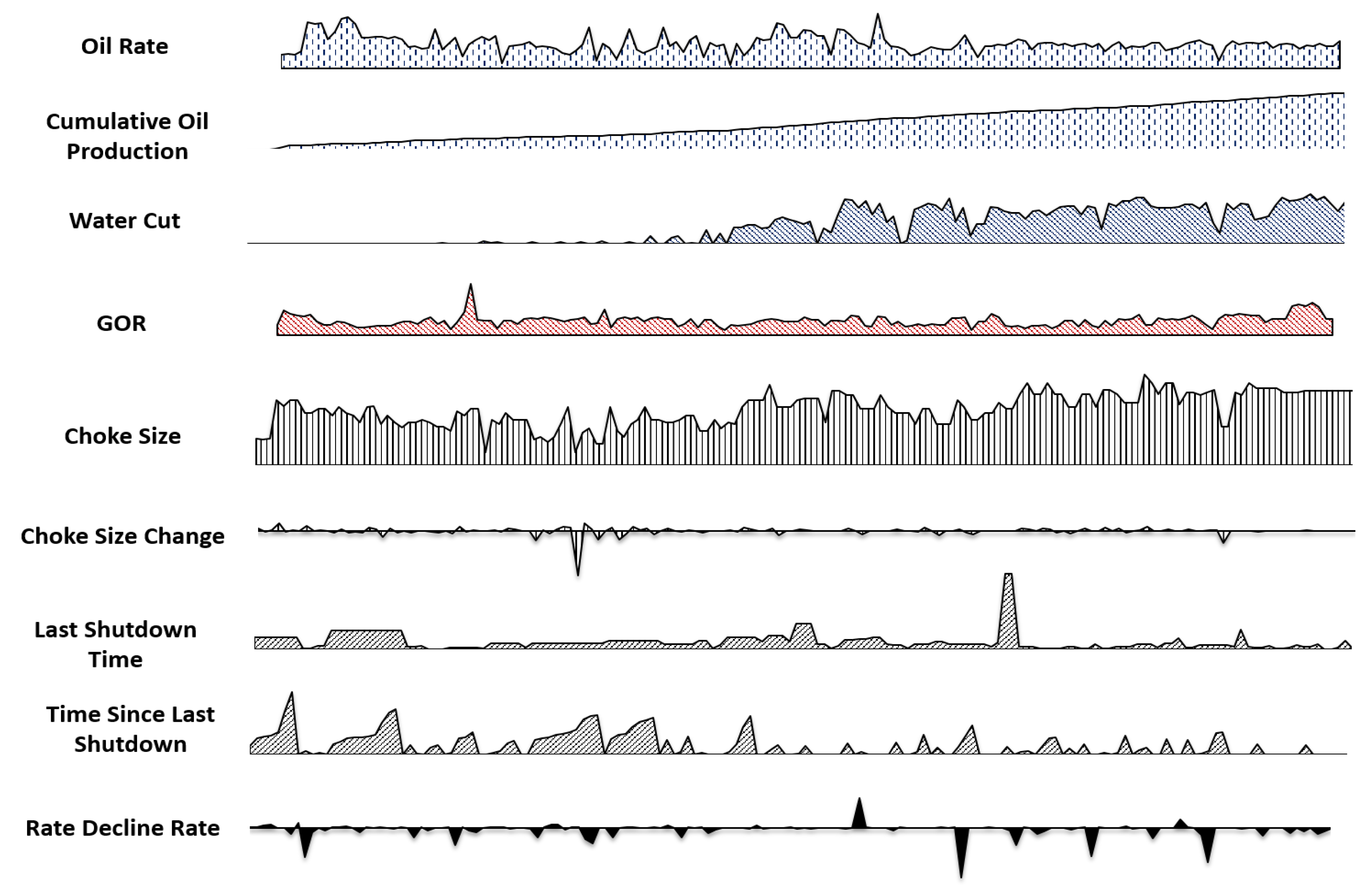
• Most reservoir surveillance data are in a multivariate time-series form with different strengths of internal correlation. Figure 1 illustrates the water cut, oil rate, shutdown status, and choke size with time for one well. If we consider predicting the decline rate of production wells, it is not just a simple function of the historical production rate. It is a function of the water cut, GOR, the change of choke size, previous shut-in period, well locations, early-or-late stages of the development, etc. It is challenging to capture and leverage the dynamic dependencies among multiple variables. To fully understand this problem, production data from many wells would have to be analyzed under varying conditions and analyzed using multivariate methods to reveal the patterns and relationships. Previous methods only keep one or limited subsets of attributes for training. For example, the traditional method of decline curve analysis (DCA) only utilizes the historical production rate data to predict the future production rate [27,28]. Engineers also integrated the surveillance data (including but not limited to bottom hole pressure measurements, pressure transient studies, production logging, pulsed neutron capture logging and flow rate measurements) by the mapping and objective method-based analysis [29]. While this makes the training easier, discarding data attributes leads to information loss and reduces the prediction accuracy and generality.

Figure 1. Historical water cut, oil rate, shutdown status and choke size for one well.

Figure 1. Historical water cut, oil rate, shutdown status and choke size for one well.

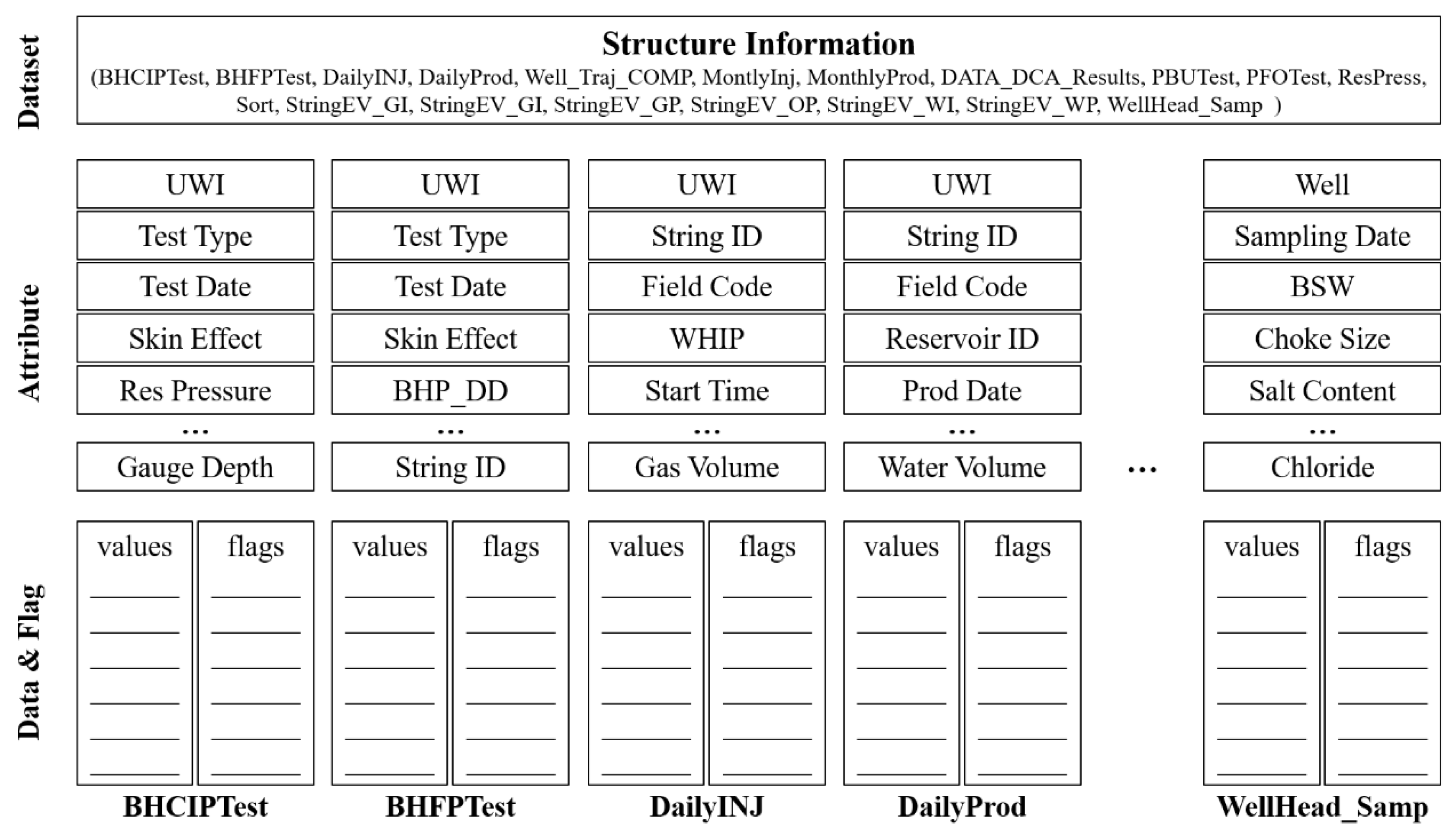
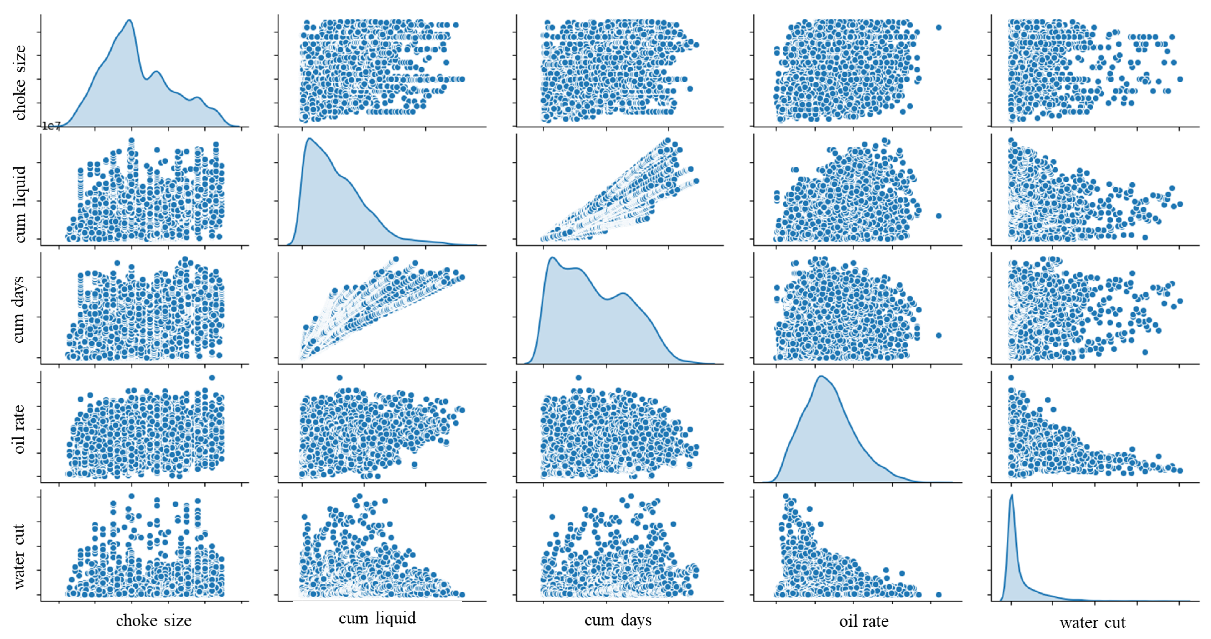
• The reservoir surveillance data contains data obtained for multiple wells (Figure 2) and from multiple sources, such as the daily injection and production monitoring, bottomhole closed-in pressure (BHCIP) test, pressure build up (PBU) test, wellhead fluid sampling, etc., as well as data of several attributes, such as the test date, WHIP, choke size, salt content, etc. (Figure 3). These attributes together provide a wealth of information for the prediction. However, it is nontrivial to use all attributes in a unified model because of variations regarding their data type. For example, the daily monitoring data such as the production rate, choke size, and water cut are in the time-series real number form. The well shut-in conditions are in the time-series Boolean form. The field code and well nameare time-independent character strings.

Figure 2. Normalized production oil rate data for multiple wells.

Figure 2. Normalized production oil rate data for multiple wells.

Figure 3. Data structure with multiple sources and attributes.

Figure 3. Data structure with multiple sources and attributes.

• Selecting a suitable machine learning algorithm for the production data forecast can also be a difficult task. It is tedious to try all available models. Many factors need to be considered in this model selection, such as explainability, the number of features and examples, the nonlinearity of the data, training speed, prediction speed, cross-validation function, etc. Each model also contains many parameters to be tuned for the best prediction performance. Industry applications typically prefer a machine learning algorithm that is capable of explanation.

The objective of the present research is to build a machine learning approach to predict the oil production rate with the reservoir surveillance data of multiple sources, forms, and attributes. It will also aim to examine the effectiveness of this novel technique in applications to the engineering problem of production data forecast. This paper is arranged as follows. In Section 2, we briefly introduce the reservoir, including its geology conditions, reservoir development strategy, as well as the production history. In Section 3, we describe the algorithm of the gradient boosted classification and regression trees and also discuss why this machine learning model is chosen to handle this engineering problem. In Section 4, long-term and short-term features are extracted from the original data to train and test the model. Further dimensionality reduction of the extracted data is also conducted by the time-segmentation technique and the polynomial regression. Last and most importantly, we show this machine learning approach is quite promising in capturing the complicated patterns between the target variable and several other explanatory variables, and thus predicting the daily oil rate in Section 5.

2. The Low-Permeability Carbonate Reservoir

The oil-bearing reservoir in this study comprises tight carbonates with low porosity and permeability [30]. Its low relief structure represents a central high with gently dipping towards the flanks. The distribution of geological facies and other reservoir properties are also relatively homogeneous. This reservoir is under development by multiple injection and production well clusters with a uniform scheme. Production interferences between different clusters are negligible due to the low reservoir permeability. Currently, three phases in the sequence are on implementation. All phases involve water alternating miscible gas injection (WAG) through an inverted 5-spot pattern with fixed well spacing. Injectors and producers with similar lateral lengths are completed as open-hole slanted horizontal wells across major subzones. Because of the similarities among these wells regarding local geology conditions and the reservoir development scheme, the ensemble of monitoring data from all producers can be utilized to train the machine learning model rather than the one-by-one well analysis.

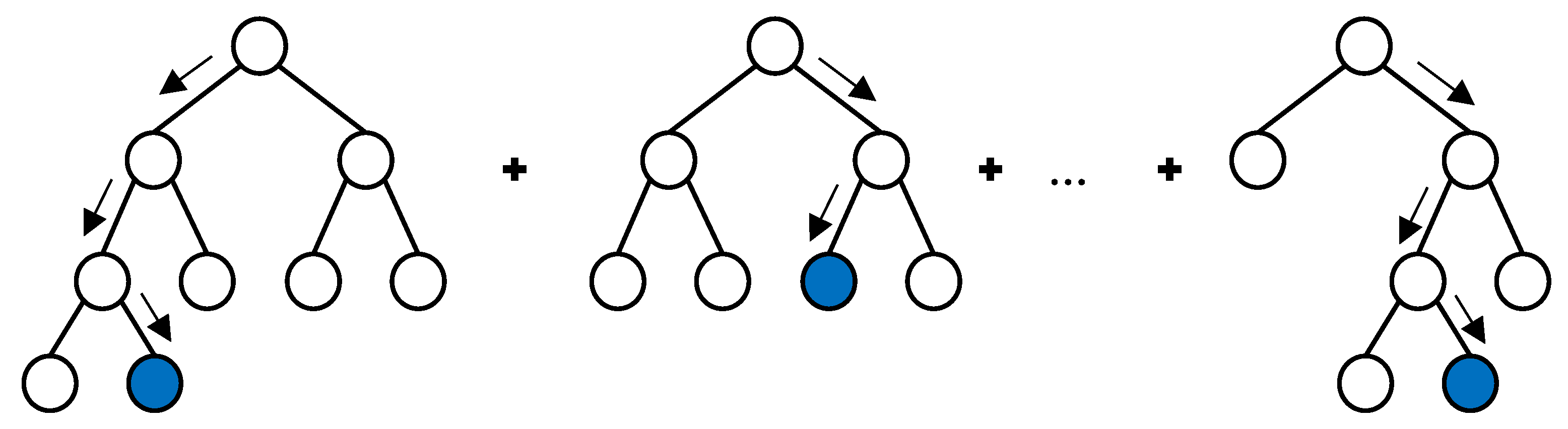
3. Gradient Boosted Classification and Regression Trees

The novel approach proposed in this work for the reservoir surveillance predicative analysis combines both the classification and regression methods. We assume the multiple linear regression can describe the dependence between the target variable (i.e., production rate decline rate) and several other explanatory variables (e.g., water cut, cumulative production, and production rate). We also assume that different temporal and spatial categories require the adoption of different regression models. The gradient boosted tree is a capable machine learning technique for regression and classification problems [31]. It produces the prediction model in the form of an ensemble of classification and regression trees, CART in short [32], in which the root and branch nodes are for classifications, and the end-leaf nodes are for regressions (Figure 4). In this work, the tree-based machine learning algorithm, instead of neural network kind of algorithm (e.g., RNN, LSTM, ConvNet), is selected for the machine learning task by considering its convenience to handle the small- or medium-sized tabular data as well as its explanation capability for industry applications.

The model is trained by the greedy method of enumerating all different tree structures, then find an optimal ensemble of tree structures with node scores [6]. Its objective is to optimize the following objective function, given the training data:

$$obj={\displaystyle \sum _{i=1}^{n}l\left(y_i,{\widehat{y}}_i^{(t)}\right)}+{\displaystyle \sum _{k=1}^t\Omega \left(f_k\right)}$$

(1)

where l is the training loss function, which is used to quantify the accuracy of the predictive target value (${{\widehat{y}}_i}^t$) with respect to the training target data ($y_i$). Ω is the regularization term to control the model complexity and avoid overfitting. The subscript i indexes over the training set of size n. The superscript t is the boosting step number. The prediction value at boosting step t is defined recursively. The result of all CARTs add up to the predicted value, and then the next CART fits the residual of the error function to the predicted value, which is the error between the predicted value and the real value:

$${\widehat{y}}_i^{(t)}={\displaystyle \sum _{k=1}^t{f}_k(x_i)}={\widehat{y}}_i^{(t-1)}+f_t(x_i)$$

(2)

which is the sum of prediction value at the last boosting step and the tree at the t step from the explanatory training variable $x_i$. The function f describes conducting classification and regression from the CART tree.

$$f_t(x)=w_{q(x)},w\in R^T,q:R^d\to \left\{1,2,\dots ,T\right\}$$

(3)

where w is the vector of scores on leaves, q is a function assigning each data point to the corresponding leaf, and T is the number of leaves. The training variable $x_i$ is composed from all its components, due to the size of training set, as introduced under Equation (1).

4. Long-Term and Short-Term Feature Extraction

Properly optimized feature extraction is key to the effective machine learning model construction [33]. The expert experiences in reservoir surveillance analysis indicate that informative features include both short-term and long-term factors. In this work, selected long-term features aim to reflect the reservoir development stage. Many reservoir engineers prefer using the concept “early stage”, “mid stage” and “late-stage” to classify the production period of an oil filed and make corresponding reservoir development plans. This is because production behaviors and multi-phase fluid flow mechanism in the subsurface of different stages may vary significantly. In the early stage, the injection and production displacement in this reservoir has not been established, and oil is produced by the natural depletion mechanism. Though reservoir pressure around producers is declining, it still remains relatively high above the saturation pressure. Free gas evolution from the dissolved gas is not observed. The breakthrough of bottom water, injected water or miscible-flooding gas has not occurred either. In the mid- or late-stage, however, reservoir pressure remains stable with the establishment of the displacement system. GOR and water cut keeps increasing after the breakthrough of the displacement front.

This “development stage” feature is representative but sort of quantitatively blurred from the perspective of data analysis because there is no direct recorded metrics reflecting this long-term feature. In this work, the cumulative oil production, water cut, and GOR are selected long-term features trying to characterize the development stage (Figure 5). Figure 5 plots variations of these features for one single well over its whole production period.

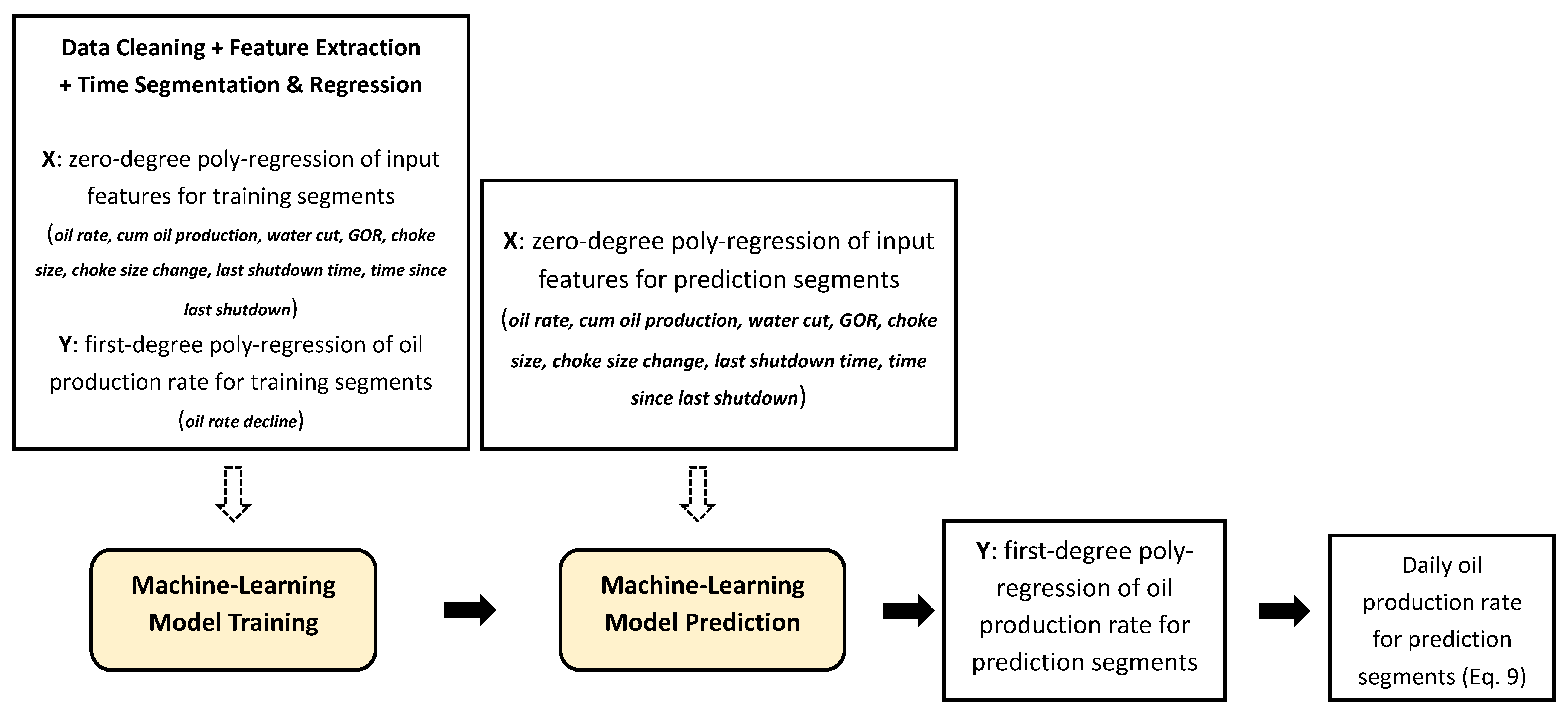
• Cumulative oil production: considering similarities among all producers regarding their local geological conditions as well as reservoir development scheme (e.g., well spacing, horizontal well length) in this oil field, their drainage amount of reserves, and total ultimate oil production are close (Section 2). The cumulative oil production at specific observation dates, therefore, can reflect percentages of recovered oil, and thus can reflect the development stage;
• Water cut and GOR: water cut is correlated to the development stage in this oil field, as can be observed in Figure 1 and Figure 5. In the early stage of reservoir development, the initial water saturation is close to the connate water saturation (Swc), water conning from the bottom water has not occurred, and the displacement front of water alternating gas (WAG) from injectors have not reached to producers. Water cut data in this stage is close to zero. Then this value begins to increase from the mid-stage because the bottom water and injected water reached to producer areas. GOR has a similar correlation trend as the water cut. In mid- or late-stages, free gas evolves from the dissolved gas with the pressure decreasing. Injected gas will also arrive nearby producers.

Note that pressure profiles, such as bottom hole pressure (BHP) or wellhead pressure (WHP), are also long-term features and may have a significant effect on predicting the decline rate. In this oil field, however, sufficient and continuously recorded data of these two pressure parameters are not available. BHP is only measured once or twice per year for selected wells to monitor the reservoir pressure distribution, and only a few wells are equipped with gauges to continuously track WHP.

Short-term fluctuations are also observed in the production data, mainly due to two operation activities: adjusting the choke size and temporal well shut-in. Choke refers to a mechanical device placed in the flow line to restrict and control the flow of oil by changing the flowing pressure. Temporally shut-in the well can help restore the reservoir pressure and mitigate the bottom-water conning. In this work, we utilize four factors “choke size”, “choke size change”, “last shutdown time”, and “time since last shutdown” to quantify these two operation activities (Figure 5).

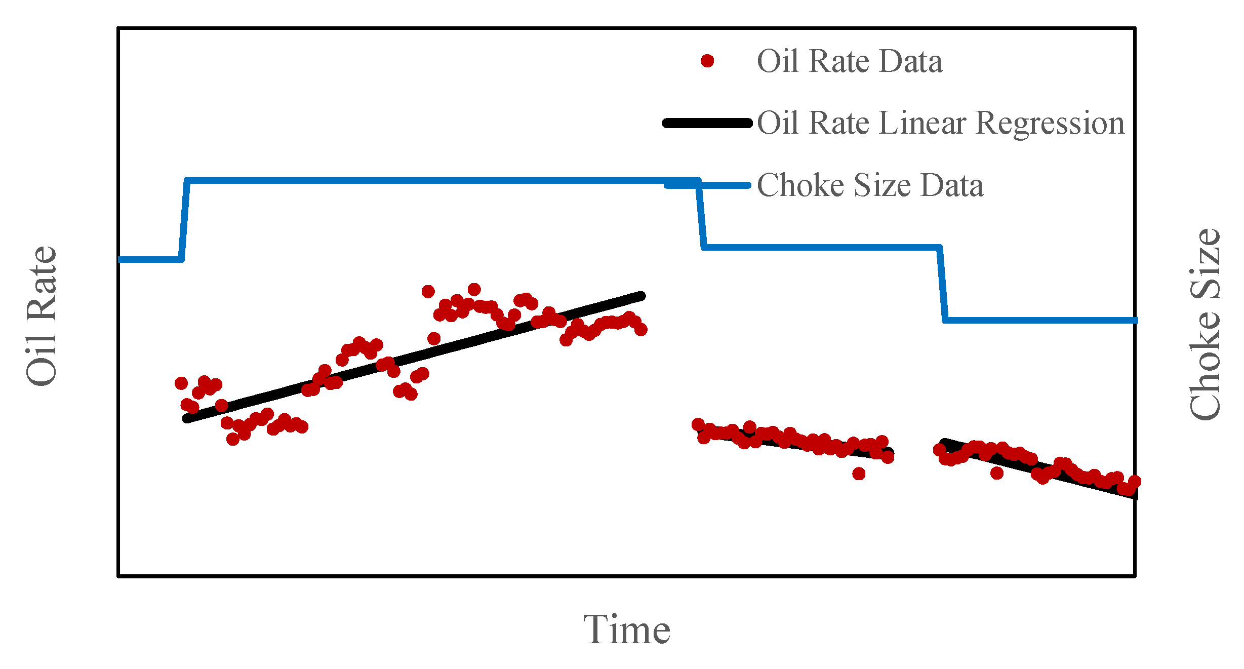
• Oil rate: oil production rate decline can be a function of current production rate according to the traditional decline curve analysis method (e.g., the hyperbolic exponent approach);
• Choke size and choke size change: adjusting the choke size is the direct operation approach to control production rate, and thus it has an influence on oil rate and oil rate decline. Our surveillance analysis experiences indicate that oil rate tends to increase more sensitively to the increase of choke size, and decrease less sensitively to the decrease of choke size in the early stage;
• Last shutdown time and time since last shut down: shutting down the producer for a while will help the pressure restoration and thus affects the production behavior;

The target prediction parameter in this algorithm is the oil rate decline (Figure 5). In the training set, this parameter is obtained by the first-order poly regression of the daily oil rate data. Predicting the future oil rate with the decline rate value from the training model and previous production rate is elaborated in Section 5.2.

• Rate decline: rate decline is the prediction target in this analysis.

Figure 6 plots the joint distribution of a few pairs of the extracted attributes. Only the first five parameters are selected for demonstration clarity. On the diagonal axes is the univariate distribution of the data for the variable in that column. It is observed that variables of the extracted features mostly follow the normal or log-normal distributions. On the off-diagonal axes are the joint distribution of the feature pairs. The joint distribution of most feature pairs is quite scattered, which indicates quantitative prediction through bivariate linear regression is impractical. A strong linear relationship is only observed between the parameter “cumulative liquid” and “cumulative days” (plot [2,3] and plot [3,2]), of which the physics behind is quite common sense.

Figure 7 summarizes the workflow of this work to predict the surveillance data with the machine-learning tree boosting method and the time-segmented feature extraction. It includes the model training, model prediction, segment extrapolation, and prediction of the daily oil rate. Details of each step are explained in the above sections.

Further dimensionality reduction of the extracted data is conducted through the technique of time segmentation and polynomial regression (Figure 8). In this way, the multiple series of extracted features on a daily basis are transferred to a list of vectors with a much smaller size [34]. In addition, noises in the daily recorded data can be eliminated, and only key trends and characteristics are captured. For example, the 81 scattered daily oil production data in the first segment of Figure 8 can be transferred to only two values (average oil rate and rate decline) with this time segmentation and polynomial regression. It indicates the oil rate is gradually climbing in this time interval with the increased choke size. Changing points for this segmentation are identified as the dates when the choke size change or when wells are shut-down/restored. For each segmentation, zero-degree polynomial regression of the given dataset is conducted to calculate the average $\overline{y}$.

$$\overline{y}=\frac{{\displaystyle \sum _{i=1}^N{y}_i}}{N}$$

(4)

where N is the number of recorded daily data within a time segment, and first-degree polynomial regression is conducted to calculate the change rate of this attribute within this time segment.

$${\widehat{y}}_i=a+b{x}_i$$

(5)

$$b=\frac{N{\displaystyle \sum _{i=1}^N{x}_i{y}_i}-\left({\displaystyle \sum _{i=1}^N{x}_i}\right)\left({\displaystyle \sum _{i=1}^N{y}_i}\right)}{N{\displaystyle \sum _{i=1}^N{x}_i^2}-{\left({\displaystyle \sum _{i=1}^N{x}_i}\right)}^2}$$

(6)

$$a=\frac{{\displaystyle \sum _{i=1}^N{y}_i}-b{\displaystyle \sum _{i=1}^N{x}_i}}{N}$$

(7)

where a and b are the line intercept and slope, respectively. ${\widehat{y}}_i$ is the regressed dependent variable. In this work, the zero-degree polynomial regression is conducted on all input features to obtain their average value for a given time segment. The first-degree polynomial regression is only conducted on the oil rate data to get the decline rate of oil production for each time segmentation, which is the target prediction parameter in this training work. It is demonstrated as the slope of regressed line segments in Figure 8. The equation to obtain this value with the discrete data in each interval is given in Equation (6).

5. Applications

The predictive model is implemented based on the XGBoost package [4], which internally employs classification and regression trees. This model is known for its high predictive performance, flexibility, robustness to outliers and unbalanced classes, and efficiency by the parallel search of the best split. In this section, we will demonstrate the effectiveness of our developed approach with two tests.

5.1. Randomly 90/10 Split and K-Fold Cross-Validations of the 91 Producer Data Assemblage

In the first test, the total dataset is the assemblage of extracted features from all 91 producers for the last 20 years. By the long- and short-term feature extraction with the time-segmentation techniques, it is transformed into the form of 8495 × 16 matrix (16 is the number of extracted features, 8495 is the number of data pieces). The preprocessed data set is then randomly divided into the training set and the evaluation set (90% for training and 10% for evaluation). In the XGBoost model, several hyper-parameters need to be tuned to improve regression performances. To find the best hyperparameters for each experiment, we performed random searches with the hyperopt Python package [35]. More specifically, the search was done with 100 sets of hyper-parameters, and the set that achieved the minimum root mean square error (RMSE) was selected. The following parameters were tuned: learning rate in the interval (0.001, 0.02); the minimum weight of a child tree is set (0, 1.0); the maximum depth of trees in (4,12); the subsampling parameter in (0.5, 1); and the number of estimators in (2000, 10000). The evaluation metric RMSE is defined as follows to evaluate our algorithm. The tuned hyper-parameters in the XGBoost model for this test are listed in

Table 1. Tuned hyper-parameters in the XGBoost model.

Parameters	Values
learning_rate	0.00283
n_estimators	16800
max_depth	7
min_child_weight	0.8715
gamma	0
subsample	0.6712
colsample_bytree	0.7
objective	reg:linear
nthread	−1
scale_pos_weight	1
seed	27
reg_alpha	0.00006

Note: Definitions of hyper-parameters can be referred in Chen and Guestrin, 2016.

.

$$\mathrm{RMSE}=\sqrt{\frac{1}{N}{\displaystyle \sum _{i=1}^N{\left({\widehat{y}}_i-y_i\right)}^2}}$$

(8)

Figure 9 shows the cross-plot between the true value and the predicted value of the oil decline rate for the evaluation dataset. The dashed line plots the equation y = x. It can be observed that our model predicts reasonably well. Most of the sample predictions are close to the realistic recording data. Compared with the scattered pattern in the joint distribution of feature pairs (Figure 6), the predictive capacity of this machine learning model is significantly improved. Some outliers seem to be clustered near one region, which indicates scenarios for these regions can be improved by a more detailed feature analysis. Prediction accuracy of this level is valuable in practice, which will be elaborated in the following section.

Different splitting of the training set and test set may cause a change in the model accuracy. The k-fold cross-validation tests are also conducted to eliminate this influence and to further check the effectiveness of this developed method. The group number in this k-fold cross-validation is set to be 5. In

Table 2. Root mean square error (RMSE) result of the randomly 90/10 split and k-fold cross-validation tests.

Test	90/10 Split	k-Fold (Group Number = 5)
		1st	2nd	3rd	4th	5th
RMSE	2.1903	2.3033	2.7689	2.5161	2.5112	2.3124

, we compared the RMSE of the randomly 90/10 split test and k-fold test. The RMSE in the k-fold test is slightly larger than the randomly 90/10 split because the hyperopt parameter in the XGBoost model (Table 1) is optimized based on the randomly 90/10 split test, as mentioned above. The cross-plot between the true value and the predicted value of the oil decline rate for the k-fold test is plotted in Figure 10. As can be observed in Figure 9 and Figure 10, there are outliers of which the deviations between the predicted values and true values are significant. This could be caused by some local geological or production scheme features, such as local geological unconformity, special well treatment, etc. In this study, only eight features are chosen as input to train the model for this real field case, some outlier predictions are within expectation. These features can be included, if needed, to improve the performance of the machine learning algorithm.

Further numerical tests with various split ratio (90/10, 70/30, 60/20/20) are conducted. The RMSE results of the testing groups are provided in

Table 3. RMSE results for various split ratio tests.

Test	Split Ratio
	90/10	80/20	70/30	60/40
RMSE	2.1903	2.3791	2.5113	2.53971

. The training error promotes slightly with the increase of training set. The error in the validation set is about twice larger than that in the training set. This indicates the selected training model may still be underfitting for the data. This makes sense from the perspective of production geology and reservoir engineering. For a real-field oil reservoir with 20 years production history, the surveillance behaviors can be influenced by thousands of factors. The CART based approach with extracted limited number of parameters in this study cannot capture all recorded features. However, it still provides prediction capability with fairly acceptable engineering tolerance, which is further discussed in the next section.

Figure 11 visualizes the trained gradient boosting decision trees, showing the features and feature values for each split as well as the output leaf nodes. Only half of the tree is plotted, and various features are marked with different colors for the clear demonstration. In Figure 11, the circular nodes (branches) demonstrate the classification in the model, and the square nodesleaves) show the regression functions. The top feature influencing the decline rate, as shown in the root node, is the choke size increment. This training result matches our experiences in analyzing the surveillance data of this reservoir. The following key features in sequence (from root node to the leaf nodes) are oil production rate, choke size, the influence of well shut-down, water cut, well index, and cumulative liquid production. Capabilities to output the trained model is one advantage of the tree-boosted machine learning method over the neural network method, because industry may prefer the model explainability instead of a black-box.

5.2. 90 Producers Data for Training and the Other 1 Producer Data for Testing

In the second test, we use the data from 90 producers to train the model and data of the left one for evaluations. The objective is to check the capacity of this machine learning model in predicting the whole-life production of a given well, with no data of this well provided. The whole production life of this evaluation well is divided into 49 segmentations with our feature extraction methods. In each segmentation, only the production rate on the first day is given, and rates in the following days are predicted. Our machine learning approach is able to output the oil decline rate (i.e., decline slope) for each segment. Equations to obtain the production rate for one specific day with associated decline rate and previous production rates are as follows:

$${\widehat{y}}_k=\{\begin{array}{c}{y}_k,k=1\\ -\frac{{\displaystyle \sum _{i=1}^{k-1}\left(b{x}_i-y_i\right)}}{k-1}+b{x}_k, k>1\end{array}$$

(9)

where $\widehat{y}$ and y denote the predicted oil rate and the recorded oil rate, respectively. x denotes the date. The subscript k represents the kth day in a given time segment. b is the predicted slope from the machine learning model. This equation can be easily derived from the least square method. Figure 12 plots the comparison between the field recorded and the predicted oil production rate for the whole life of this well. In comparison, we also conducted numerical tests with two other approaches. The first approach uses the local linear regression. The second approach combines the time segmentation technique with an estimated decline rate by assuming its uniform distribution. History matching performances of these three approaches are compared in Figure 12. It can be observed that results by combining the machine learning decline rate and the time segmentation technique achieve much better results than the other two approaches. The accuracy of this model prediction is also demonstrated by computing the percentage of production rate, of which the predicted value is within 5%, 10%, and 20% of the field recorded value, as listed in

Table 4. Error distributions between the prediction and true values for three methods.

Method	Within 5% of Production Rate	Within 10% of Production Rate	Within 20% of Production Rate
LocalLinearRegress	10.00%	33.91%	85.27%
TimeSeg + EstDecline	37.61%	57.65%	77.82%
TimeSeg + MLDecline	58.08%	84.35%	96.36%

.

6. Summary and Discussions

• We present a machine-learning tree boosting method and the time-segmented feature extraction technique for the predictive analysis of the reservoir surveillance data. This approach aims to quantitatively uncover the complicated hidden patterns between the target prediction parameter and other monitored data of a high variety through state-of-the-art automatic classification and multiple linear regression algorithms. Compared with traditional methods, the approach proposed in this article can handle surveillance data in multivariate time-series form with different strengths of internal correlation. It also provides capabilities for data obtained in multiple wells, measured from multiple sources, as well as of multiple attributes. Manually constructing such a model—considering features of this complexity—would be challenging.
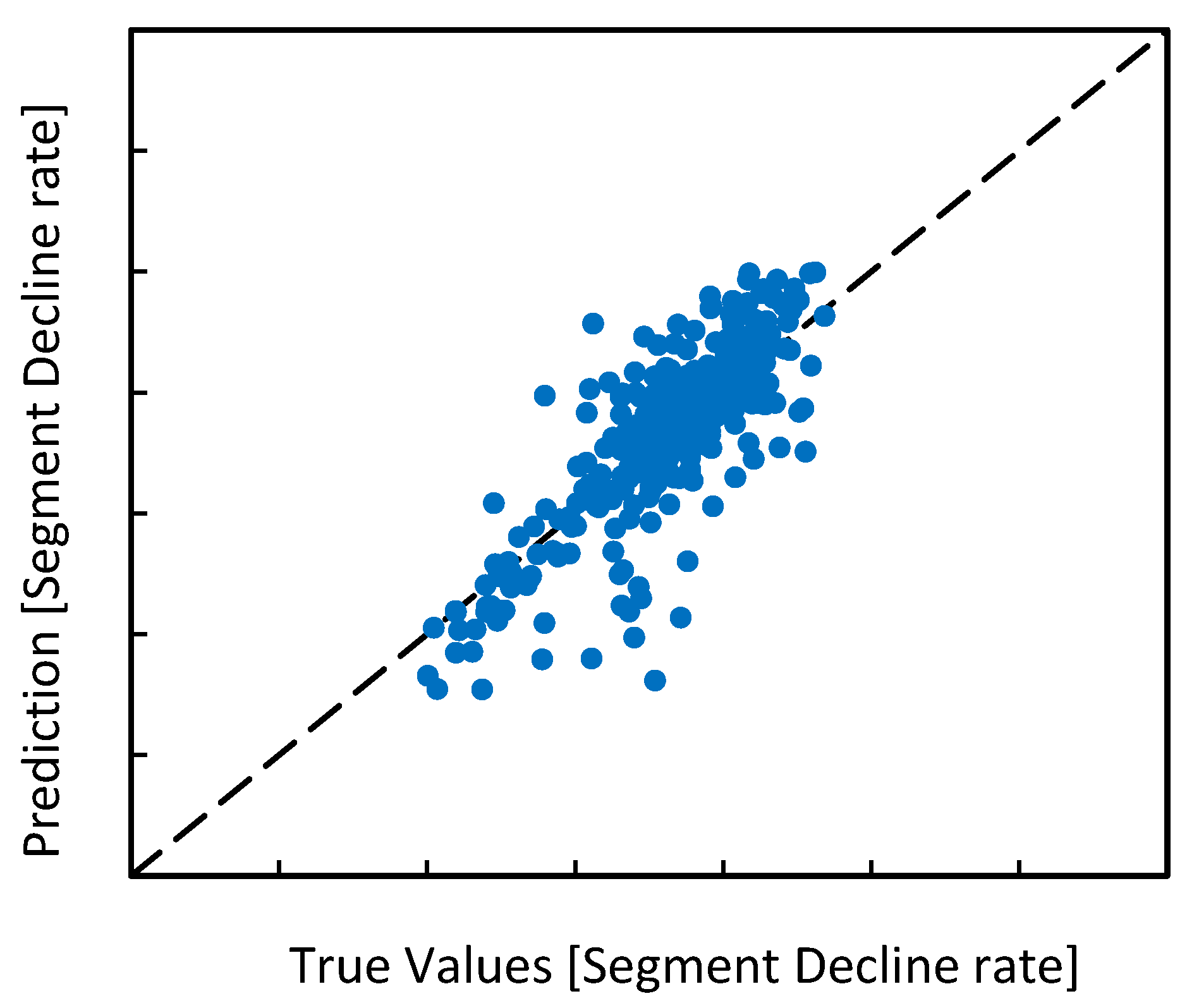
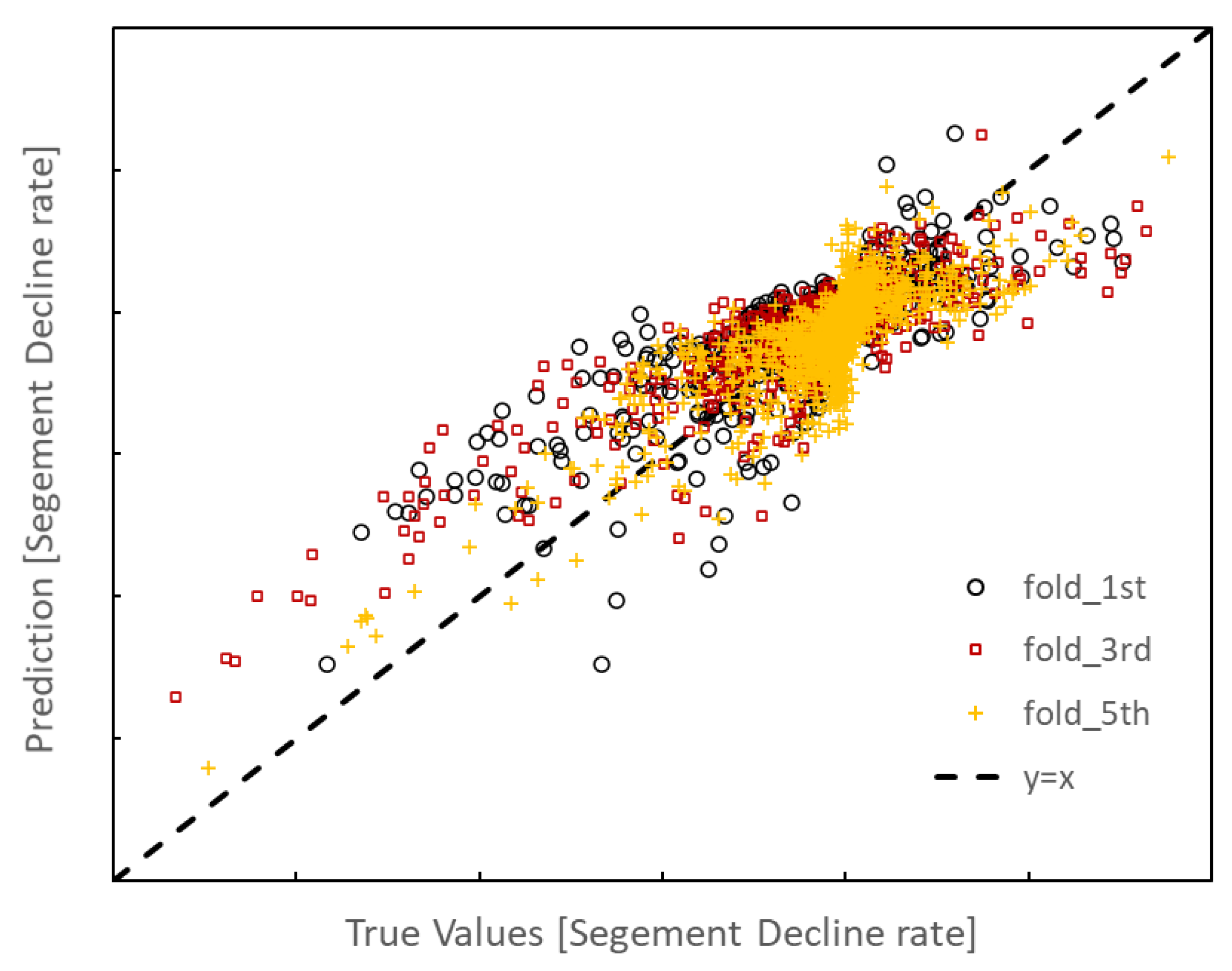
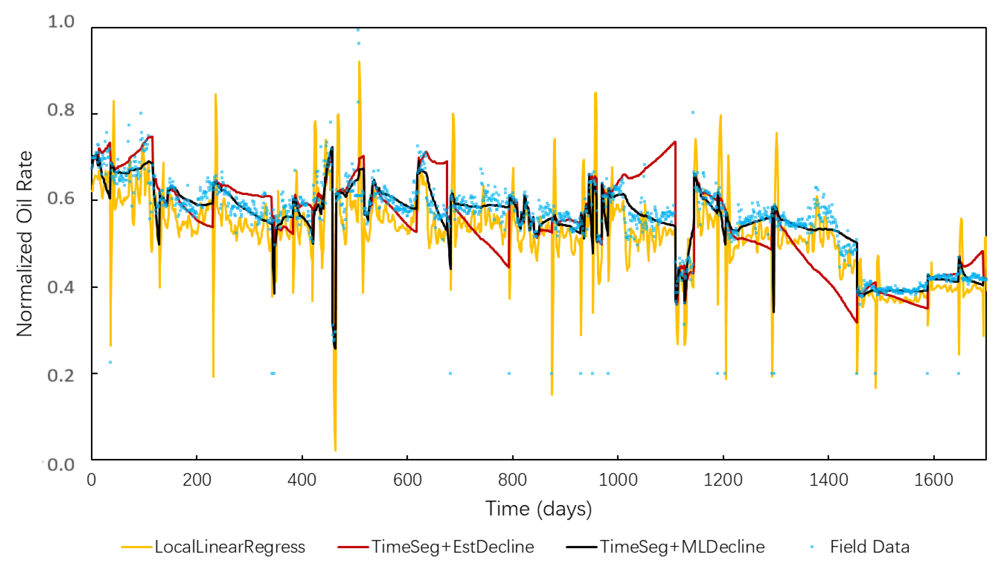
• The developed approach is applied to a field case with 91 producers and 20 years of development history. Two tests are conducted. In the first test, the preprocessed data set of all 91 producers is randomly divided into the training set and the evaluation set. The prediction performance is checked through the cross-plot between the true value and predicted value of the oil decline rate. An RMSE of 2.1903 can be achieved by the proposed method. In the second test, data of 90 producers are used in training, and the left one is for evaluations. We show 96.36% of the predicted data is within 20% error of realistic recording data, which brings 18.54% improvement of accuracy and reliability compared with other approaches.
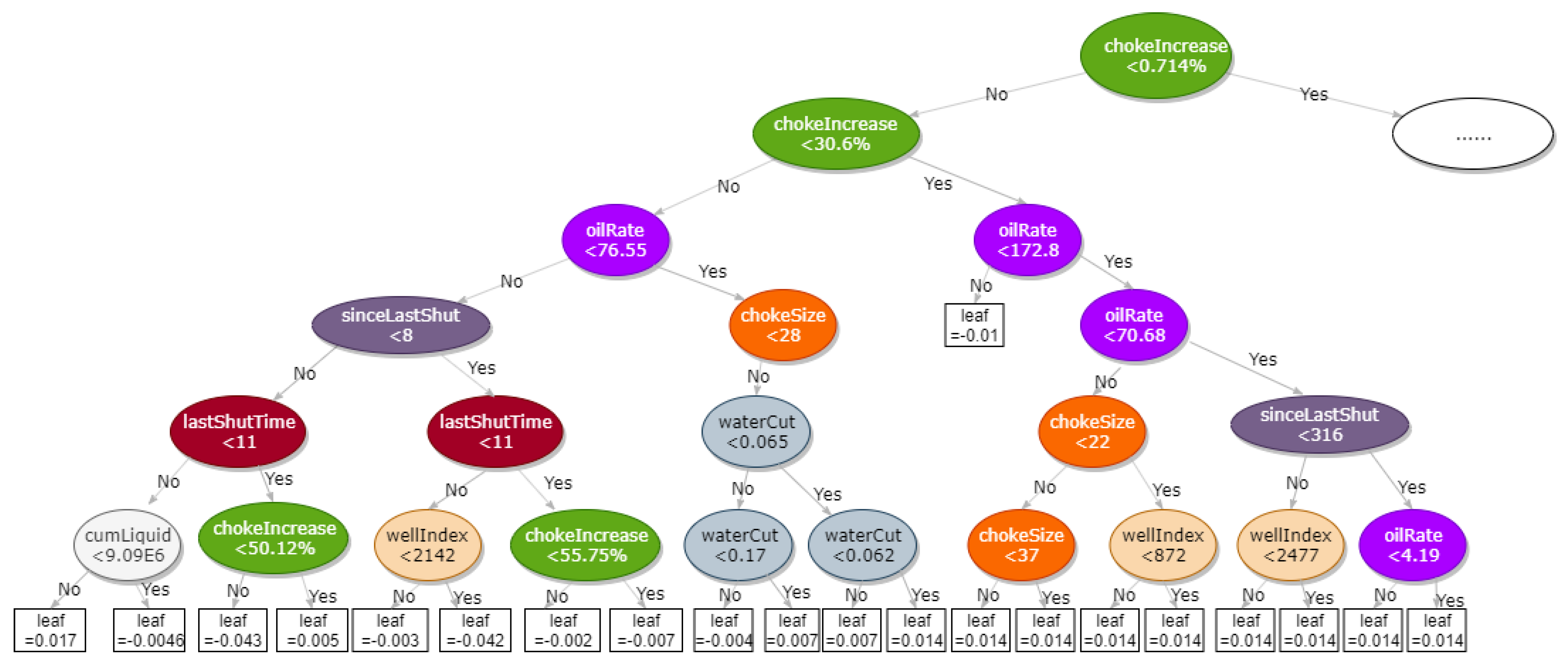
• Long-term features reflecting the development stages (e.g., the cumulative oil production, water cut, and GOR), and short-term fluctuations by two operation activities (well shut-down and choke size adjustment) can be considered in this model. According to our test, the influential features in sequence are the choke size change, oil production rate, current choke size, the well shut-down status, water cut, well location, and cumulative liquid production.
• Our application results indicate that this approach is quite promising in capturing the complicated patterns between the target variable and several other explanatory variables of the surveillance data, and thus in predicting the daily oil production rate. Continuing work based on this machine learning framework could potentially help in better managing the fields and reducing the maintenance cost, e.g., identifying in advance some possible failure of equipment and to intervene before an event occurs
• Features of local geology conditions and the reservoir development scheme are not included in the model training in this research, because of the homogeneous geological conditions and uniform development pattern in this oil field. Notice only eight features are chosen as the input to train the model for this real field case; some outlier predictions are within expectation. One machine learning model including geological and production features is recommended to be more practical in general. Some smart-model based approaches may also be valuable to extract training features. In addition, more sensitivity analysis of the input parameters can be done based on the proposed ML model. The model is expected to be more reliable and accurate if more valuable features are included.

References

1. Terrado, R.M.; Yudono, S.; Thakur, G.C. Waterflood Surveillance and Monitoring: Putting Principles into Practice. In Proceedings of the SPE Annual Technical Conference and Exhibition, San Antonio, TX, USA, 24–27 September 2006; Society of Petroleum Engineers: Dallas, TX, USA, 2006. [Google Scholar]
2. Shalev-Shwartz, S.; Ben-David, S. Understanding Machine Learning: From Theory to Algorithms; Cambridge University Press: Cambridge, UK, 2014. [Google Scholar]
3. Bishop, C.M. Neural Networks for Pattern Recognition; Oxford University Press: Oxford, UK, 1995. [Google Scholar]
4. LeCun, Y.; Bottou, L.; Bengio, Y.; Haffner, P. Gradient-based learning applied to document recognition. Proc. IEEE 1998, 86, 2278–2324. [Google Scholar] [CrossRef] [Green Version]
5. He, K.; Zhang, X.; Ren, S.; Sun, J. Deep Residual Learning for Image Recognition. In Proceedings of the IEEE Conference on Computer Vision And Pattern Recognition, Las Vegas, NV, USA, 26 June–1 July 2016; pp. 770–778. [Google Scholar]
6. Chen, T.; Guestrin, C. Xgboost: A scalable tree boosting system. In Proceedings of the 22nd Acm Sigkdd International Conference on Knowledge Discovery and Data Mining, San Francisco, CA, USA, 13–17 August 2016; Association for Computing Machinery: New York, NY, USA, 2016; pp. 785–794. [Google Scholar]
7. Alkinani, H.H.; Al-Hameedi, A.T.T.; Dunn-Norman, S.; Flori, R.E.; Alsaba, M.T.; Amer, A.S. Applications of Artificial Neural Networks in the Petroleum Industry: A Review. In Proceedings of the SPE Middle East Oil and Gas Show and Conference, Manama, Bahrain, 18–21 March 2019; Society of Petroleum Engineers: Dallas, TX, USA, 2019. [Google Scholar]
8. Xu, C.; Misra, S.; Srinivasan, P.; Ma, S. When Petrophysics Meets Big Data: What can Machine Do? In Proceedings of the SPE Middle East Oil and Gas Show and Conference, Manama, Bahrain, 18–21 March 2019; Society of Petroleum Engineers: Dallas, TX, USA, 2019. [Google Scholar]
9. Poulton, M.M. Neural networks as an intelligence amplification tool: A review of applications. Geophysics 2002, 67, 979–993. [Google Scholar] [CrossRef]
10. Alizadeh, B.; Najjari, S.; Kadkhodaie-Ilkhchi, A. Artificial neural network modeling and cluster analysis for organic facies and burial history estimation using well log data: A case study of the South Pars Gas Field, Persian Gulf, Iran. Comput. Geosci. 2012, 45, 261–269. [Google Scholar] [CrossRef]
11. Ross, C. Improving resolution and clarity with neural networks. In SEG Technical Program Expanded Abstracts; Society of Exploration Geophysicists: Houston, TX, USA, 2017; pp. 3072–3076. [Google Scholar]
12. Arabloo, M.; Bahadori, A.; Ghiasi, M.M.; Lee, M.; Abbas, A.; Zendehboudi, S. A novel modeling approach to optimize oxygen–steam ratios in coal gasification process. Fuel 2015, 153, 1–5. [Google Scholar] [CrossRef]
13. Sidaoui, Z.; Abdulraheem, A.; Abbad, M. Prediction of Optimum Injection Rate for Carbonate Acidizing Using Machine Learning. In Proceedings of the SPE Kingdom of Saudi Arabia Annual Technical Symposium and Exhibition, Dammam, Saudi Arabia, 23–26 April 2018; Society of Petroleum Engineers: Dallas, TX, USA, 2018. [Google Scholar]
14. Kamari, A.; Bahadori, A.; Mohammadi, A.H.; Zendehboudi, S. Evaluating the unloading gradient pressure in continuous gas-lift systems during petroleum production operations. Petrol. Sci. Technol. 2014, 32, 2961–2968. [Google Scholar] [CrossRef]
15. Chamkalani, A.; Zendehboudi, S.; Bahadori, A.; Kharrat, R.; Chamkalani, R.; James, L.; Chatzis, I. Integration of LSSVM technique with PSO to determine asphaltene deposition. J. Petrol. Sci. Eng. 2014, 124, 243–253. [Google Scholar] [CrossRef]
16. Rashidi, M.; Asadi, A. An Artificial Intelligence Approach in Estimation of Formation Pore Pressure by Critical Drilling Data. In Proceedings of the 52nd US Rock Mechanics/Geomechanics Symposium, Seattle, WA, USA, 17–20 June 2018; American Rock Mechanics Association: Houston, NV, USA, 2018. [Google Scholar]
17. Dzurman, P.J.; Leung, J.Y.W.; Zanon, S.D.J.; Amirian, E. Data-Driven Modeling Approach for Recovery Performance Prediction in SAGD Operations. In Proceedings of the SPE Heavy Oil Conference-Canada, Calgary, AB, Canada, 11–13 June 2013; Society of Petroleum Engineers: Dallas, TX, USA, 2013. [Google Scholar]
18. Chang, H.; Zhang, D. Identification of physical processes via combined data-driven and data-assimilation methods. J. Comput. Phys. 2019, 393, 337–350. [Google Scholar] [CrossRef] [Green Version]
19. Zendehboudi, S.; Rezaei, N.; Lohi, A. Applications of hybrid models in chemical, petroleum, and energy systems: A systematic review. Appl. Energy 2018, 228, 2539–2566. [Google Scholar] [CrossRef]
20. Wang, C.; Ran, Q.; Wu, Y.S. Robust implementations of the 3D-EDFM algorithm for reservoir simulation with complicated hydraulic fractures. J. Petrol. Sci. Eng. 2019, 181, 106229. [Google Scholar] [CrossRef]
21. Wang, C.; Winterfeld, P.; Johnston, B.; Wu, Y.S. An embedded 3D fracture modeling approach for simulating fracture-dominated fluid flow and heat transfer in geothermal reservoirs. Geothermics 2020, 86, 101831. [Google Scholar] [CrossRef]
22. Wang, C.; Huang, Z.; Wu, Y.S. Coupled numerical approach combining X-FEM and the embedded discrete fracture method for the fluid-driven fracture propagation process in porous media. Int. J. Rock Mech. Min. Sci. 2020. [Google Scholar] [CrossRef]
23. Wu, Y.S.; Li, J.; Ding, D.; Wang, C.; Di, Y. A generalized framework model for the simulation of gas production in unconventional gas reservoirs. SPE J. 2014, 19, 845–857. [Google Scholar] [CrossRef]
24. Chang, O.; Pan, Y.; Dastan, A.; Teague, D.; Descant, F. Application of Machine Learning in Transient Surveillance in a Deep-Water Oil Fieldc. In Proceedings of the SPE Western Regional Meeting, San Jose, CA, USA, 23–26 June 2019; Society of Petroleum Engineers: Dallas, TX, USA, 2019. [Google Scholar]
25. Pan, Y.; Bi, R.; Zhou, P.; Deng, L.; Lee, J. An Effective Physics-Based Deep Learning Model for Enhancing Production Surveillance and Analysis in Unconventional Reservoirs. In Proceedings of the Unconventional Resources Technology Conference, Denver, CO, USA, 22–24 July 2019; pp. 2579–2601. [Google Scholar]
26. Al-Fattah, S.M.; Startzman, R.A. Neural network approach predicts US natural gas production. SPE Product. Facil. 2003, 18, 84–91. [Google Scholar] [CrossRef]
27. Fetkovich, M.J. Decline Curve Analysis Using Type Curves. In Proceedings of the Fall Meeting of the Society of Petroleum Engineers of AIME, Las Vegas, NV, USA, 30 September–3 October 1973; Society of Petroleum Engineers: Dallas, TX, USA, 1973. [Google Scholar]
28. Agarwal, R.G.; Gardner, D.C.; Kleinsteiber, S.W.; Fussell, D.D. Analyzing Well Production Data Using Combined Type Curve and Decline Curve Analysis Concepts. In Proceedings of the SPE Annual Technical Conference and Exhibition, New Orleans, LA, USA, 27–30 September 2014; Society of Petroleum Engineers: Dallas, TX, USA, 2014. [Google Scholar]
29. Sinha, S.P.; Al-Qattan, R. A Novel Approach to Reservoir Surveillance Planning. In Proceedings of the Abu Dhabi International Conference and Exhibition, Abu Dhabi, EAU, 10–13 October 2004; Society of Petroleum Engineers: Dallas, TX, USA, 2004. [Google Scholar]
30. Saadawi, H.N. Commissioning of Northeast Bab (NEB) Development Project. In Proceedings of the Abu Dhabi International Petroleum Exhibition and Conference, Abu Dhabi, EAU, 5–8 November 2006; Society of Petroleum Engineers: Dallas, TX, USA, 2006. [Google Scholar]
31. Friedman, J.H. Greedy function approximation: A gradient boosting machine. Ann. Stat. 2001, 29, 1189–1232. [Google Scholar] [CrossRef]
32. Breiman, L.; Friedman, J.; Stone, C.J.; Olshen, R.A. Classification and Regression Trees; CRC Press: Boca Raton, FL, USA, 1984. [Google Scholar]
33. Domingos, P. A few useful things to know about machine learning. Commun. ACM 2012, 55, 78–87. [Google Scholar] [CrossRef] [Green Version]
34. Keogh, E.; Chu, S.; Hart, D.; Pazzani, M. Segmenting time series: A survey and novel approach. In Data Mining In Time Series Databases; World Scientific Publishing: Singapore, Singapore, 2004; pp. 1–21. [Google Scholar]
35. Bergstra, J.; Komer, B.; Eliasmith, C.; Yamins, D.; Cox, D.D. Hyperopt: A python library for model selection and hyperparameter optimization. Comput. Sci. Discov. 2015, 8, 014008. [Google Scholar] [CrossRef]
Figure 4. Illustration of the classification and regression trees (CARTs) ensembles.
Energies 13 06307 g004
Figure 5. Extracted long-term (cumulative oil production, water cut, gas oil ratio (GOR)) and short-term time-series features (oil rate, choke size, choke size change, last shutdown time, and time since the last shutdown).
Energies 13 06307 g005
Figure 6. Joint distribution of a few pairs of extracted features.
Energies 13 06307 g006
Figure 7. Workflow to predict the surveillance data with the machine-learning tree boosting method and the time-segmented feature extraction.
Energies 13 06307 g007
Figure 8. Time segmentation based on choke size change and well shut-down and data regression.
Energies 13 06307 g008
Figure 9. The cross-plot between the true value and the predicted value of the oil decline rate with the 90/10 split.
Energies 13 06307 g009
Figure 10. The cross-plot between the true value and the predicted value of the oil decline rate with k-fold cross validation test (k = 5).
Energies 13 06307 g010
Figure 11. Trained CART structures demonstrating key features for interpretations.
Energies 13 06307 g011
Figure 12. Comparison between the field recorded data and the machine learning predicted data for the whole life of one producer.
Energies 13 06307 g012