Abstract
The tip clearance has an important effect on the performance of an engine compressor. While the impact of tip clearance on a concentric compressor has been widely explored in previous research, the flow field distribution of an eccentric compressor has only been minimally explored. Both the steady and unsteady computational fluid dynamics (CFD) methods have been widely used in the studies of concentric axial-compressors, and they have similar simulation results in terms of flow field. However, they have been rarely applied to axial-compressors with non-uniform tip clearance to investigate their flow field. In this paper, ANSYS CFX is used as CFD software, and both steady and unsteady CFD methods are applied to study a single rotor of ROTOR67 to investigate the compressor characteristic line and flow field under different eccentricity conditions. The results show that non-uniform tip clearance creates a non-uniform flow field at the inlet and tip regions over the whole operating range. The circumferential position where the flow coefficient and the axial velocity are the smallest occurs at a position close to the maximum tip clearance and is located on the side deviating toward the direction of rotation of the rotor. Compared with steady CFD, unsteady CFD has better predictive capability for the flow field distribution in axial compressors with non-uniform tip clearance.
1. Introduction
A lot of experiments and numerical simulation show that tip clearance plays an important role [1,2,3] in the performance and stability of axial compressors. However, a large number of published literature studies are based on axial compressors with uniform tip clearance, which may not fully reveal the true physical laws. In practice, non-uniform tip clearance is inevitable in the production, processing, assembly and long-term use of axial flow compressors.
The common forms of non-uniform tip clearance can be divided into two categories [4]. The first category is a static non-uniform tip clearance, which is mainly caused by rotor eccentricity or casing deformation, as shown in Figure 1. The non-uniform tip clearance can be described by ε = ε(θ), where ε is the tip clearance and θ is the circumferential coordinate; the second type is the dynamic non-uniform tip clearance, mainly due to the difference in blade height or the rotor swirling motion caused by Alford force and vibration force, as shown in Figure 2.The non-uniform blade height and swirling motion of the rotor can be defined as ε = ε(θ − ωt) and ε = ε(θ − υt), respectively, where O is the center of the rotor, O’ is the center of the casing, and the reference system is the geodetic coordinate system.
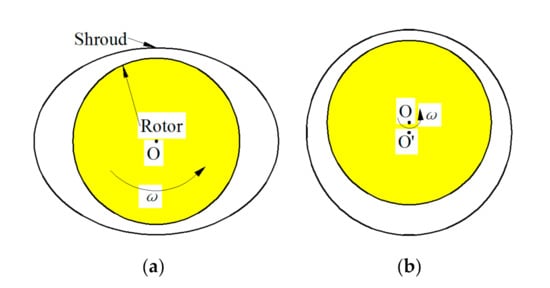
Figure 1.
Static non-uniform tip clearance. (a) Ovalized casing; (b) eccentric rotor [4].
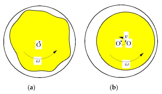
Figure 2.
Dynamic non-uniform tip clearance. (a) Non-uniform blade height; (b) whirling rotor [4].
The influence of tip clearance on the performance and stability of axial compressors is a classic academic problem, which has attracted so many pioneering scholars [5,6,7,8]. However, compared with the study of uniform tip clearance, the research on non-uniform tip clearance is relatively recent. In 1997, Graf [9] first developed a two-dimensional model for predicting the effect of non-uniform tip clearance on the performance of axial compressors, as shown in equation 1. He put forward that the local total-to-static pressure rise coefficient (ψ) is a function of local flow coefficient (φ) as well as of local tip clearance (ε), and his model was verified by Wong’s [10] experiments. The model did not consider the radial flow field.
where λ is an inertia parameter related to compressor geometry:
Then Song [11] combined the continuity equation, axial and circumferential momentum equations with two shock disk models to analyze the effect of non-uniform tip clearance on compressor blade load. After 2000, with the introduction of active control and stall warning, more and more researchers have conducted experiments to investigate the relationship between non-uniform tip clearances and stall signals. For example, Cameron [12] investigated the effect of non-uniformity of tip clearance on stall signal detection. In addition, Morris [13] shifted the compressor rotor with a tip clearance value of 24%, and studied the propagation law of the stall signal in experiments. He found short length-scale disturbances grew at the location with a large tip clearance, and decayed in the tighter tip clearance sector of the compressor. The eccentricity produced clear changes in stall inception behavior. In 2012, Young [14] conducted an experimental study on blade passing signature analysis in eccentric compressors. By analyzing the irregularity of the pressure signals at different circumferential positions, it was found that the signal irregularity of the position with a small gap is small, and the signal irregularity with a large gap is large. In addition, the experimental results showed that the test compressor, with design average tip clearance, exhibited spike-type stall inception in both concentric and eccentric configurations. However, the modal wave was observed in both concentric and eccentric configurations with mid-sized average clearances. The tip clearance and eccentricity were found to affect the stall inception mechanism of the compressor (spike or modal) [15]. When the tip clearance increased, the mechanism of stall initiation was unclear. Corresponding to that, Teng Cao [16] developed a three-dimensional Immersed Boundary Model with Smeared Geometry (IBMSG) solver which used a Euler code and loss correlation to predict the behavior of an eccentric compressor given its concentric performance. The detailed description of IBMSG can be seen in reference [16].
Because of the complexity of the axial-compressor with a non-uniformity of tip clearance, most of the above studies focus on experimental research. However experimental research cannot obtain the detailed field information and flow mechanism. Although many scholars have developed numerical models for calculating non-uniform tip clearance flow, such as Graf model [9] and IBMSG [16]. However, these models are simplified methods and inseparable from the modification of loss and experiment data, which also can not reveal the unsteady flow mechanism, such as pre-stall and stall inception etc. With the development of computers, the calculation of the full-annulus of the compressor has become a possibility, so many scholars have begun to use CFD to research the intake distortion [17,18,19,20] and the unsteady tip leakage flow [21,22] of axial compressors. Recently, some scholars [23,24,25] have also begun to use CFD to study the flow field distribution and performance of non-uniform tip clearance on axial compressors. However, these scholars [24] have not paid attention to the difference between the steady CFD and unsteady CFD methods in calculating the flow in an axial-compressor with non-uniform tip clearance, and have not given the reasonable circumferential flow field distribution. Therefore, the problem needs to be explained reasonably. In this paper, flow field in axial compressors with non-uniform tip clearance will be simulated by steady and unsteady methods, and a comparison will be made to explain the reason causing different results between the steady and unsteady methods.
In fact, the non-uniform distribution of the tip clearance along the circumferential direction is often caused by complex conditions, which makes it difficult to study. In order to simplify the complexity of the non-uniform tip clearance, the eccentricity is considered as a typical form of non-uniform tip clearance in this paper. In addition, the Cambridge scholar Anna M.Young [15] has also conducted detailed experimental studies on eccentric compressors, and the results of this experiment can also verify the relevant conclusions in this paper. Therefore, the calculations in this paper are only focused on the numerical calculation of the eccentric case.
2. Research Object and Numerical Method
2.1. Research Object and Definition of Eccentricity
NASA rotor 67 [26] was chosen as the test case in this paper. The main reason for this choice is the relatively large tip clearance, which is helpful for the mesh quality of the eccentric compressor, especially in the case of large eccentricity. In addition, there is a large amount of public experimental data [26] that can be accessed.
This paper takes the ROTOR67 single rotor as the research object and adopts steady and unsteady CFD methods to calculate and study the eccentric compressor with three kinds of eccentricity under three working conditions of near chock (NC), near peak efficiency (NPE) and near stall (NS), respectively. The specific parameters of the single rotor are shown in Table 1.

Table 1.
Main design parameters of Rotor67.
In order to quantitatively analyze the non-uniform tip clearance, the eccentricity [14] is defined as shown in Figure 3. In particular, the case of E = 0 corresponds to concentric compressors, and the case of E > 0 corresponds to eccentric compressors.
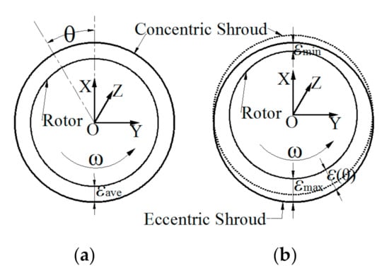
Figure 3.
Schematic diagram of concentric compressor and eccentric compressor. (a) Concentric compressor; (b) eccentric compressor.
Figure 4 is a distribution diagram of the tip clearance along the circumferential direction with 0% eccentricity, 80% eccentricity and 160% eccentricity, respectively. The distribution of the tip clearance of the eccentric compressor along the circumferential direction is approximately a cosine function. For the case of 80%, the maximal tip clearance is 1.4 mm, and the minimal is 0.6 mm. For the 160%, the maximal and the minimal gaps are 1.8 mm and 0.2 mm, respectively.
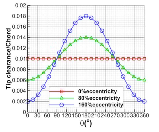
Figure 4.
The circumferential distribution curve of the tip clearance for different eccentricities.
Table 2 shows the specific values of the maximum tip clearance and the minimum tip clearance of the compressor in the case of three eccentricities. According to previous studies [14], the eccentricity of most axial compressors is 50% to 75%.
Table 2.
The maximum and minimum clearance for different eccentricities.
2.2. Numerical Methods and Validation
The schematic diagrams of the computational domain and mesh are shown in Figure 5a–f. In order to consider the unsteady effect of the rotor blade and the non-uniform tip clearance during the rotor rotation, this paper divided the grid into two parts, as shown in Figure 5b. The Inner Domain and The Outer Domain were generated by the Turbo Grid and ICEM (Integrated Computer Engineering and manufacturing code for Computational Fluid Dynamics)mesh generator, respectively. The 3D sector of the Whole domain is shown in Figure 5f. Figure 5g,h are the view of the domain in the axial direction, and the geometry of outer domain was adjusted with different eccentricity to achieve different grids. In order to ensure that the computational results are independent of the grid distribution, mesh studies were conducted in the 0% eccentricity case of steady calculation. Three grid systems, Grid A, Grid B and Grid C were tested. The total numbers of nodes for Grid A, Grid B and Grid C were approximately 12 million, 15 million and 20 million, respectively. The detailed information about these grid systems is shown in Table 3 and Table 4. I, J and K are the circumferential direction, the radial direction and the axial direction, respectively. According to the ICEM criterion, the grid quality of outer domain is around 1. For the inner mesh domain, the minimum skewness, the maximal aspect ratio and the expansion ratio are 29, 3541.1 and 3.1, respectively. In order to ensure the accuracy of the flow field at the tip of the blade, over 20 mesh nodes were given in the radial direction of the rotor tip clearance region for all cases.
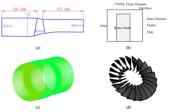
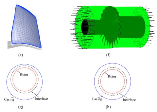
Figure 5.
Schematic diagram of the grid and computational domain. (a) The length of the inlet and outlet duct; (b) whole domain; (c) the mesh in outer domain; (d) inner rotor mesh; (e) the grid on the rotor blade; (f) three-dimensional sector of the whole domain; (g) the geometry for concentric case; (h) the geometry for eccentric case.
Table 3.
Mesh statistic for 1 passage in the inner domain.
Table 4.
Mesh statistic in the outer domain.
In this paper, the CFX software package in ANSYS commercial software solver was adopted. According to the previous research results of a large number of scholars [23,27], the k-ε turbulence model can accurately simulate the flow structure at the tip of the blade and the scalable wall function was selected. No-slip conditions were imposed at solid boundaries. Atmospheric conditions for total pressure (101,325 Pa) and total temperature (288.15 K) are defined as the boundary conditions at the rotor inlet along with turbulence intensity of 5%. At the outlet plane, average static pressure is imposed. By increasing the static pressure of the outlet plane, the performance of the rotor is obtained. To investigate the effect of steady and unsteady CFD methods for eccentric compressor research, the interface boundary condition is given in two ways: (1) the frozen rotor method, which is widely used for data transmission between the rotor and stator interface of the concentric compressor. (2) The Transient Rotor Stator Method, which is widely used for data transmission between the compressor rotor and stator interface in the unsteady CFD. The numerical divergence point is used as the criterion for determining the instability of the compressor. Figure 6 shows the calculated and experimental results of the relative Mach number in the near peak efficiency point (NPE) at the design speed and 1.016 mm uniform tip clearance. It can be seen from Figure 6 that the calculated results are in good agreement with the relative Mach numbers of the experimental results at the point of NPE. This shows that the computational simulation has considerable reliability.
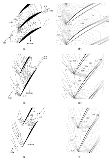
Figure 6.
The Mach number (Ma) of the calculated and experimental value at the point of near peak efficiency (NPE). (a) 30% Span Experiment; (b) 30% Span Computation; (c) 70% Span Experiment; (d) 70% Span Computation; (e) 90% Span Experiment; (f) 90% Span Computation.
The computed total pressure ratio and adiabatic efficiency are plotted against normalized mass flow and compared with experimental data in Figure 7. It can be seen from Figure 7 that the total pressure ratio curve and the experimental data are quite different, and the stall flow coefficient at the near stall boundary also has a certain difference, but the efficiency curve agrees well with the experimental data. The relative deviations for the total pressure ratio at near choke condition (NC), near peak efficiency condition (NPE) and near stall condition (NS) are 1.5%, 1.8% and 3.2%, respectively, and for efficiency are 2.3%, 0.2% and 0.8%, respectively. The relative deviation for the flow coefficient at the stall point is 2.2%. Figure 8 shows the radial distribution of the total pressure ratio and total temperature ratio downstream of the rotor NPE. The computed exit total temperature agrees very well with the measurement along the span, but the computed exit total pressure is somewhat low near the hub and becomes progressively better towards the tip. Moreover, as shown in Figure 7, the characteristic lines with three grids are approximately consistent. Therefore, when the number of grids is greater than Grid A, the results are independent in grid density. Accounting for the amount of computing time, the Grid B is adopted in the following study.
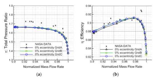
Figure 7.
Comparison of experimental and calculated characteristic lines. (a) Total pressure ratio characteristic line; (b) total efficiency characteristic line.
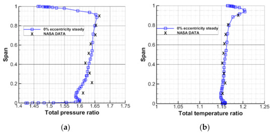
Figure 8.
Comparison of experimental and calculated spanwise distributions of total pressure ratio, total temperature ratio at the point of NPE. (a) Spanwise distribution of total pressure ratio; (b) spanwise distribution of total temperature ratio.
The differences between CFD and experimental data can be found in the previous literature. For example, Dario Bruna and Mark G. Turner [28] found that the stability boundary of numerical calculations and experimental results are quite different when calculating ROTOR37. When Yingxiu Chen [23] calculated ROTOR67, they found that the total pressure ratio and the flow rate at the stall point also show some errors regarding experimental data. It is difficult to avoid due to the limitations [29,30] of CFD.
3. Numerical Simulation Results and Discussion
3.1. Characteristic Line Calculation and Analysis
In order to save computing time and cost, the characteristic line is often obtained by a steady CFD method. For example, the multi-stage axial flow compressor is essentially an unsteady flow, but in engineering, the characteristic line is often calculated by a steady CFD method. Therefore, the calculation of the characteristic line in this paper is based on the method of steady CFD calculation. However, unsteady CFD calculations were only carried out in three working conditions, NC, NPE and NS.
Figure 9 is a characteristic line obtained by the steady CFD calculation method in the case of different eccentricities. By comparing the characteristic lines of different eccentricities, it can be found that the eccentricity has different effects on the total pressure ratio, efficiency and stability boundary. The eccentricity has the most obvious effect on the stability boundary.
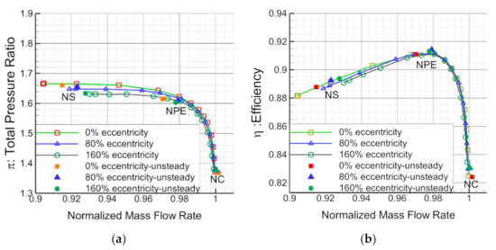
Figure 9.
Effect of eccentricity on the performance curve. (a) Effect of eccentricity on the total pressure ratio; (b) effect of eccentricity on the efficiency.
3.2. Influence of Non-Uniform Tip Clearance on the Distribution Law of Flow Field
3.2.1. Influence of Non-Uniform Tip Clearance on Distribution of Inlet Flow Coefficient
Taking E = 160% as an example, the flow coefficient distribution of the inlet section is analyzed under different eccentric conditions. The inlet section in this paper is taken from plane L1 (as shown in Figure 5a), which is one rotor chord upstream of the rotor inlet plane. The coordinate system and the definition of θ analyzed below are shown in Figure 3. Flow coefficient can be defined as below.
Figure 10 is a contour plot showing the distribution of flow coefficients at L1 for both steady and unsteady CFD near choke (NC). It can be seen from Figure 10a,b that the flow coefficient calculated by the two CFD methods is relatively uniform in the circumferential direction at the NC. Comparing the Figure 10a,b, it can be seen that the region where the flow coefficient is larger in the steady CFD result is on the right side of the x-axis, while the region where the flow coefficient is larger in the unsteady CFD result is mainly concentrated on the upper side of the y-axis. The difference of the calculated flow coefficient between the steady and unsteady CFD methods is not obvious.
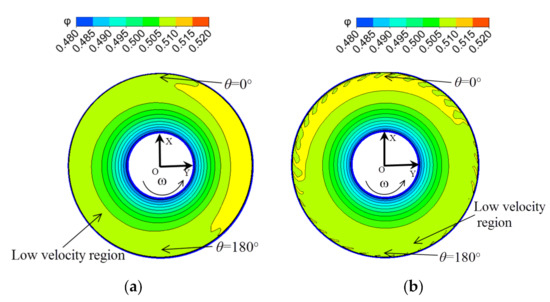
Figure 10.
Distribution of inlet flow coefficient near chock (NC) in the case of E = 160%. (a) Steady computational fluid dynamics (CFD) result; (b) unsteady CFD result.
Figure 11 is the contour plot of the inlet flow coefficient for both steady and unsteady CFD at NPE. It can be seen from Figure 11a,b that the flow coefficient calculated by the steady and unsteady CFD methods has become non-uniform along the circumferential direction at NPE. Comparing the Figure 11a,b, the region where the flow coefficient is small in the steady CFD result is on the left side of the maximum tip gap position, and the region where the flow coefficient is small in the unsteady CFD result is on the right side of the maximum tip gap position. There are obvious differences between the steady and the unsteady CFD results for flow coefficients.
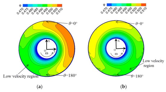
Figure 11.
Distribution of inlet flow coefficient NPE in the case of E = 160%. (a) Steady CFD result; (b) unsteady CFD result.
Figure 12 is a contour plot of the flow coefficient distribution for steady and unsteady CFD under near stall conditions. It can be seen from Figure 12a,b that under the near stall condition, the flow coefficients calculated by steady and unsteady CFD have become extremely significant non-uniform values in the circumferential direction of the inlet section. Comparing Figure 12a,b, the region where the flow coefficient is low in the steady CFD result is on the left side of the maximum tip gap position, and the region where the flow coefficient is low in the unsteady CFD result is on the right side of the maximum tip gap position. The difference between the steady and unsteady CFD calculated flow coefficient contour maps is extremely obvious, almost corresponding to two physical laws.
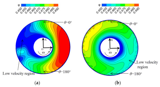
Figure 12.
Distribution of inlet flow coefficient near stall in the case of E = 160%. (a) Steady CFD result; (b) unsteady CFD result.
As shown in Figure 13, in order to quantitatively analyze the distribution law of the flow coefficient in the circumferential direction, a full-circle compressor is divided into 22 sub-compressors with equal circumferential angles equally distributed in the circumferential direction. The 22 sub-compressors represent 22 circumferential positions, each of which represents a circumferential angle. In the following analysis, the abscissa represents the position of 22 sub-compressors with θ, and each sub-compressor corresponds to a flow coefficient. The definition of θ is shown in Figure 3.
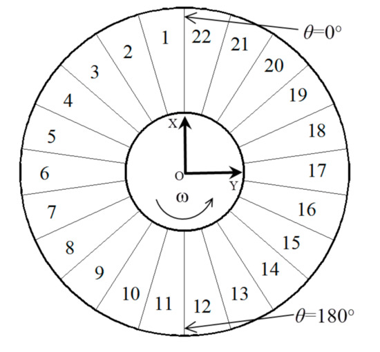
Figure 13.
Circumferential distribution of sub-compressors.
The flow coefficients of the sub-compressors along the circumference are analyzed below. In addition, the following analysis includes three eccentricity cases: 0% eccentricity, 80% eccentricity, and 160% eccentricity.
Figure 14 is a distribution of the flow coefficient along the circumferential direction in the case of 0% eccentricity. From the results of Figure 14a,b, under the three conditions of 0% eccentricity, the flow coefficients calculated by the steady and unsteady CFD are uniform in the circumferential direction.
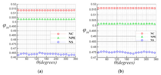
Figure 14.
Distribution of inlet flow coefficient along the circumference in the case of 0% eccentricity. (a) Steady CFD result; (b) unsteady CFD result.
Figure 15 is a distribution of the flow coefficient along the circumference in the case of 80% eccentricity. It can be seen that the flow coefficient calculated by the steady and unsteady CFD are approximately the same in the circumferential direction at NC. In the NPE and NS operating conditions, comparing Figure 15a,b, it can be found that the region with low flow coefficients in the steady CFD is on the left side of the 180°, and the area with low flow coefficient in the unsteady CFD is on the right side of the 180°, and the results of NS are more obvious.
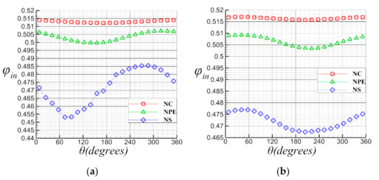
Figure 15.
Distribution of inlet flow coefficient along the circumference in the case of 80% eccentricity. (a) Steady CFD result; (b) unsteady CFD result.
Figure 16 is a distribution of flow coefficients along the circumference in the case of 160% eccentricity. From the results of Figure 16a,b, the flow coefficient of the 160% eccentricity is similar to that in the 80% eccentricity case, and becomes more pronounced.
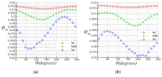
Figure 16.
Distribution of inlet flow coefficient along the circumference in the case of 160% eccentricity. (a) Steady CFD result; (b) unsteady CFD result.
3.2.2. Influence of Non-Uniform Tip Clearance on Relative Mach Number Distribution at Tip Section
Figure 17 and Figure 18 are contour plots of relative Mach number at 99% span, which are calculated from steady and unsteady CFD methods under different working conditions when E = 160%. It can be seen from Figure 17 and Figure 18, as the operating point gradually moves from the NC point to the NS point, the non-uniformity of the relative Mach number distribution in the circumferential direction of the tip clearance region is enhanced. In addition, at the near stall point, a serious blockage occurred in a certain area in the circumferential direction. Comparing Figure 17 with Figure 18, it can be seen that the low Mach number regions obtained by steady CFD are all on the left side of 180°, while the unsteady results are on the right side of 180°.
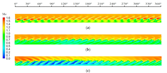
Figure 17.
The circumferential distribution of the blade tip Mach number calculated by steady CFD under different working conditions at E = 160%. (a) NC; (b) NPE; (c) near stall (NS).
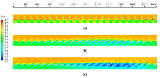
Figure 18.
The circumferential distribution of the blade tip Mach number calculated by unsteady CFD under different working conditions at E = 160%. (a) NC; (b) NPE; (c) NS.
3.2.3. Influence of Non-Uniform Tip Clearance on Axial Velocity Coefficient Distribution at Tip Section
Figure 19 and Figure 20 show the axial velocity coefficient at 99% span for different operating conditions and CFD methods when E = 160%. From Figure 19 and Figure 20, the blade tip axial velocity coefficient distributions are consistent with the distribution of the relative Mach numbers in the tip clearance region in Figure 17 and Figure 18.
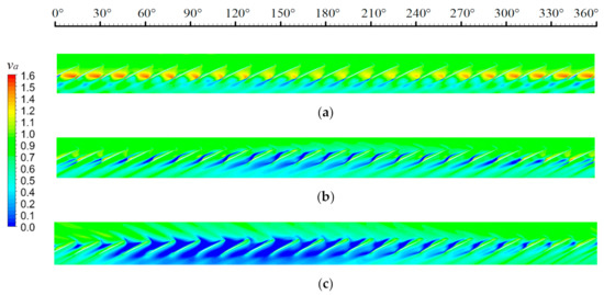
Figure 19.
The circumferential distribution of the blade tip axial velocity coefficient calculated by steady CFD under different working conditions at E = 160%. (a) NC; (b) NPE; (c) NS.
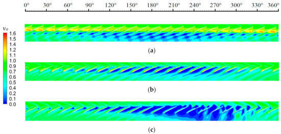
Figure 20.
The circumferential distribution of the blade tip axial velocity coefficient calculated by unsteady CFD under different working conditions at E = 160%. (a) NC; (b) NPE; (c) NS.
4. Summary and Analysis
By analyzing the results of steady and unsteady calculations, it can be seen that the non-uniform tip clearance has a great influence on the distribution of the inlet flow coefficient, the axial velocity coefficient and the relative Mach number along the circumferential direction. It is obvious that when the eccentricity is not zero, the steady and unsteady CFD results are significantly different at the NS point. In the inlet section and the tip clearance area, the minimum flow coefficient region and the minimum axial velocity region calculated by the steady CFD are both on the left of the maximum tip clearance position, whereas the minimum flow coefficient region and the minimum axial velocity region calculated by the unsteady CFD are both on the right side of the maximum tip clearance position. For a real eccentric compressor rotor, under the condition of near-stall point, what is the flow coefficient distribution of the eccentric compressor in the inlet and blade tip regions?
For this problem, foreign scholars have conducted in-depth experimental and simulation studies in recent years. Anna M.Young [15], a Cambridge scholar, has measured the circumferential distribution of the flow coefficient at the inlet section of an eccentric low-speed axial compressor. Teng Cao [16] obtained the contour plot of flow coefficient distribution on the inlet section of the low-speed eccentric compressor at the point of NS by IBMSG model. By summarizing the experimental results of foreign scholars and analyzing the results of steady and unsteady CFD in this paper, it can be concluded that the flow field obtained by unsteady CFD method in this paper is correct, while the flow field distribution calculated by steady CFD method is unreasonable.
Why are there two different results when this situation is simulated with the steady and unsteady CFD method? This will be briefly explained below, and the following analysis can be extended to all axial compressors.
Velocity triangle formula is as follows:
Projecting the above equation into the direction of the blade velocity, the above equation becomes:
Both sides of the equation are multiplied Δt, and the equation becomes the following.
In the case of steady CFD calculation, as shown in Figure 21, when the frozen rotor method is adopted, the position of the rotor relative to the casing is unchanged. After the calculation of n steps, the circumferential position of the 22 blades is unchanged. Since the steady calculation method is the time advancement method, as shown in Figure 21, and because the larger gap will produce the stronger tip leakage vortex, it is assumed here that there is a low axial velocity gas micelles named A at the 180° circumferential position (maximum tip clearance position) during the process of calculation. Since its axial velocity is considerably low, the movement of A (the low axial velocity gas micelles) in the axial and radial directions is ignored here, so that A is only considered to move in the circumferential direction. After calculating n steps, A can produce a circumferential absolute displacement using Equation (7).
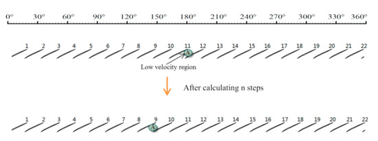
Figure 21.
Changes in the computational domain of the rotor under steady calculation.
Since the calculation domain of the blade does not rotate during the calculation, the circumferential position relative to the casing does not change. Therefore, in the steady calculation process, the displacement UΔt generated by the rotor domain implicated motion is equal to zero.
Wu is the projection of the relative velocity of A relative to the rotor blade in the direction of U. Considering the axial intake, from the knowledge of the velocity triangle, we can find that Wu is opposite to U. If the rotor blade moves in the positive direction, that is to say, then the direction of the SA is negative, so A moves to the left side of 180°. The displacement of A represents the tendency of the low-energy leakage flow, so in the case of steady calculations, the low-energy fluid will be collected on the left side of 180°. Therefore, in the case of steady CFD, the regions with the smallest flow coefficient and the lowest axial velocity are always on the left of the maximum tip clearance position.
In the case of unsteady CFD calculations, the position of the rotor blade relative to the casing is varied during the process of calculation due to the transient rotor stator boundary condition. As shown in Figure 22, after the n-step, the circumferential position of the 22 blades is understood to change. Assuming that there is a low axial velocity gas micelle named A at the 180° circumferential position (maximum tip clearance position), the movement of A in the axial and radial directions is neglected due to the low axial velocity. We only analyze A moving in the circumferential direction. After calculating n steps, after Δt, using Equation (3), A can produce a circumferential absolute displacement as follows:
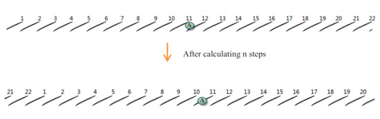
Figure 22.
Changes in the computational domain of the rotor under unsteady calculation.
Since the blade calculation domain has a rotational motion during the calculation process, the displacement term UΔt > 0 generated by the rotor domain implicated motion during the unsteady calculation process.
From the knowledge of the velocity triangle, it can be seen that the directions of Wu and U are opposite, and ; if the direction of motion of the rotor blade is positive, then
From the velocity triangle relationship, and when the gas micelle enters the rotor blade channel, it can be concluded that Cu > 0, and , so, therefore
Then the direction of the SA is positive, so A moves to the right side of 180°. SA represents the movement of low-energy leakage flow, so in the case of unsteady CFD calculations, low-energy fluids are collected on the right side of 180°. Therefore, in the case of unsteady CFD calculations, the region with the smallest mass flow rate and the smallest axial velocity are on the right side of the maximum tip clearance position.
Through the above analysis, we can find that when the eccentric compressor is calculated by the steady CFD method, since there is no implicated motion of the calculation domain, the circumferential movement direction of the low energy tip leaking gas cluster is determined by the direction of Wu. Therefore, in the case of steady CFD calculations, the region with the smallest mass flow rate is on the left of the maximum tip clearance position. However, when the eccentric compressor is calculated by the unsteady CFD method, the circumferential motion direction of the low energy tip leaking gas micelles is determined by the direction of U + Wu in the calculation process due to the implicated motion of the rotor domain. In addition, ; therefore, the direction of the circumferential movement of the low energy tip leaking gas micelles is determined by the direction of U. Therefore, in the case of unsteady CFD calculations, the circumferential position where the flow coefficient is the smallest must occur at a position located on the side deviating toward the direction of rotation of the rotor.
5. Conclusions
In this paper, ROTOR67 was taken as the research object. The three eccentricity compressors were calculated by the steady and the unsteady CFD calculation methods. The following conclusions can be drawn and extended to all axial compressors.
The eccentricity has different effects on the total pressure ratio, efficiency and stability boundary, and the effect on the stability boundary is the most pronounced.
When the eccentricity is not zero, there is obvious different results between the steady calculation and the unsteady calculation at the near stall point. In the inlet section and the tip clearance region, the minimum flow coefficient region calculated by the steady CFD method is on the left of the maximum tip clearance position. However, the minimum flow coefficient region calculated by the unsteady CFD method is on the right of the maximum tip clearance position.
For an axial compressor with an eccentricity greater than zero, it will produce a circumferentially non-uniform flow field in the inlet section or the rotor tip clearance region. In addition, the circumferential position where the flow coefficient and the axial velocity are the smallest must occur at a position close to the maximum tip clearance and located on the side deviating toward the direction of rotation of the rotor.
When simulating the flow in axial compressors with a non-uniform tip clearance, the steady CFD method has obvious defects, and the unsteady CFD has better predictive capability for the flow field distribution in axial compressors with non-uniform tip clearance.
Author Contributions
Conceptualization, C.J.; methodology, C.J.; software, C.J., J.W., and L.C.; validation, C.J., J.W., and L.C.; formal analysis, C.J. and J.H.; investigation, C.J., J.W., and L.C.; resources, J.H.; writing—original draft, C.J. and J.W.; supervision, J.H.; project administration, J.H.; funding acquisition, J.H. All authors have read and agreed to the published version of the manuscript.
Funding
The research presented here was funded by the National Science and Technology Major Project of China, grant number [2017-II-0004-0017].
Acknowledgments
The authors would like to acknowledge the supports of the National Science and Technology Major Project of China.
Conflicts of Interest
The author(s) declared no potential conflicts of interest with respect to the research, authorship, and/or publication of this article.
Nomenclature
| Symbols | |
| ε | Tip clearance |
| θ | Circumferential coordinate/direction |
| ω | Angular speed |
| t | Time |
| ν | Whirl rotating speed |
| Ma | Relative Mach number |
| Φ | Flow Coefficient |
| Ψ | Total-to-static pressure rise coefficient |
| Λ | Tnertia of fluid in rotor |
| W | Axial velocity |
| U | Rotor blade speed |
| Ρ | Air density |
| ρref | Reference density |
| Axial velocity coefficient | |
| C | Velocity in stationary frame |
| W | Velocity in rotating frame |
| S | Absolute displacement |
| Subscripts | |
| Mid | Mid-span value |
| max/min | Maximum/minimum |
| u | The direction of the blade velocity |
| in | Inlet |
| Abbreviations | |
| CFD | Computational fluid dynamics |
| NC | Near choke |
| NPE | Near Peak efficiency |
| NS | Near stall |
| IBMSG | Immersed Boundary Model with Smeared Geometry |
References
- Smith, L.H., Jr. The effect of tip clearance on the peak pressure rise of axial-flow fans and compressors. ASME Symp. Stall. 1958, 149, 152. [Google Scholar]
- Storer, J.A.; Cumpsty, N.A. An approximate analysis and prediction method for tip clearance loss in axial compressors. J. Turbomach. 1994, 116, 648–656. [Google Scholar] [CrossRef]
- Wisler, D.C. Loss reduction in axial-flow compressors through low-speed model testing. J. Eng. Gas Turbines Power 1985, 107, 354–363. [Google Scholar] [CrossRef]
- Gordon, K.A. Three-Dimensional Rotating Stall Inception and Effects of Rotating Tip Clearance Asymmetry in Axial Compressors; Diss. Massachusetts Institute of Technology: Cambridge, MA, USA, 1999. [Google Scholar]
- Lakshminarayana, B. Methods of predicting the tip clearance effects in axial flow turbomachinery. J. Basic Eng. 1970, 92, 467–480. [Google Scholar] [CrossRef]
- Chima, R.V. Calculation of Tip Clearance Effects in a Transonic Compressor Rotor; American Society of Mechanical Engineers: Birmingham, UK, 1996; Volume 78729. [Google Scholar]
- Suder, K.L.; Celestina, M.L. Experimental and computational investigation of the tip clearance flow in a transonic axial compressor rotor. J. Turbomach. 1996, 118, 218–229. [Google Scholar] [CrossRef]
- Inoue, M.; Kuroumaru, M. Structure of tip clearance flow in an isolated axial compressor rotor. J. Turbomach. 1989, 111, 250–256. [Google Scholar] [CrossRef]
- Graf, M.B.; Wong, T.S.; Greitzer, E.M.; Marble, F.E.; Tan, C.S.; Shin, H.W.; Wisler, D.C. Effects of Non-Axisymmetric Tip Clearance on Axial Compressor Performance and Stability. In Turbo Expo: Power for Land, Sea, and Air; American Society of Mechanical Engineers: Orlando, FL, USA, 1997; Volume 78682. [Google Scholar]
- Wong, T.S. Effects of Asymmetric Tip Clearance on Compressor Performance and Stability; Diss. Massachusetts Institute of Technology: Cambridge, MA, USA, 1996. [Google Scholar]
- Song, S.J.; Kil, Y.P. Rotordynamic effects of compressor rotor-tip clearance asymmetry. AIAA J. 2001, 39, 1347–1353. [Google Scholar] [CrossRef][Green Version]
- Cameron, J.D.; Bennington, M.A.; Ross, M.H.; Morris, S.C.; Corke, T.C. Effects of Steady Tip Clearance Asymmetry and Rotor Whirl on Stall Inception in an Axial Compressor. In Proceedings of the ASME Turbo Expo 2007: Power for Land, Sea, and Air, Parts A and B, Montreal, QC, Canada, 14–17 May 2007; Volume 6, pp. 457–468. [Google Scholar]
- Morris, S.C.; Cameron, J.D.; Bennington, M.A.; McNulty, G.S.; Wadia, A. Performance and short length-scale disturbance generation in an axial compressor with non-uniform tip clearance. In Proceedings of the ASME Turbo Expo: Power for Land, Sea, and Air, Berlin, Germany, 9–13 June 2008; Volume 43161. [Google Scholar]
- Young, A.; Ivor, D.; Graham, P. Stall warning by blade pressure signature analysis. J. Turbomach. 2013, 135, 011033. [Google Scholar] [CrossRef]
- Young, A.; Cao, T.; Day, I.J.; Longley, J.P. Accounting for eccentricity in compressor performance predictions. J. Turbomach. 2017, 139, 091008. [Google Scholar] [CrossRef]
- Cao, T.; Paul, H.; Paul, G.T. Hierarchical immersed boundary method with smeared geometry. J. Propuls. Power 2017, 33, 1151–1163. [Google Scholar] [CrossRef]
- Fidalgo, V.; Jerez, C.A.; Colin, Y. A study of fan-distortion interaction within the nasa rotor 67 transonic stage. J. Turbomach. 2012, 134, 051011. [Google Scholar] [CrossRef]
- Yao, J.; Gorrell, S.E.; Wadia, A.R. High-fidelity numerical analysis of per-rev-type inlet distortion transfer in multistage fans—Part I: Simulations with selected blade rows. J. Turbomach. 2010, 132, 041014. [Google Scholar] [CrossRef]
- Yao, J.; Gorrell, S.E.; Wadia, A.R. High-fidelity numerical analysis of per-rev-type inlet distortion transfer in multistage fans—Part II: Entire component simulation and investigation. J. Turbomach. 2010, 132, 041015. [Google Scholar] [CrossRef]
- Zhang, W.; Vahdati, M. A parametric study of the effects of inlet distortion on fan aerodynamic stability. J. Turbomach. 2019, 141, 011011. [Google Scholar] [CrossRef]
- Wang, Z.; Lu, B.; Liu, J.; Hu, J. Numerical simulation of unsteady tip clearance flow in a transonic compressor rotor. Aerosp. Sci. Technol. 2018, 2, 193–203. [Google Scholar] [CrossRef]
- Mao, X.; Liu, B.; Tang, T.; Zhao, H. The impact of casing groove location on the flow instability in a counter-rotating axial flow compressor. Aerosp. Sci. Technol. 2018, 76, 250–259. [Google Scholar] [CrossRef]
- Chen, Y.; Hou, A.; Zhang, M.; Li, J.; Zhang, S. Effects of Nonuniform Tip Clearance on Fan Performance and Flow Field. In Turbo Expo: Power for Land, Sea, and Air; American Society of Mechanical Engineers: Montreal, QC, Canada, 2015; Volume 56635. [Google Scholar]
- Chen, Y.; Hou, A.; Wang, W.; Zhang, M. Performance estimation method for nonuniform tip clearance cases. J. Propuls. Power 2018, 34, 1355–1363. [Google Scholar] [CrossRef]
- Kumar, S.S.; Alone, D.B.; Thimmaiah, S.M.; Mudipalli, J.R.R.; Ganguli, R.; Kandagal, S.B.; Jana, S. Aerodynamic characterization of a transonic axial flow compressor stage–with asymmetric tip clearance effects. Aerosp. Sci. Technol. 2018, 82, 272–283. [Google Scholar] [CrossRef]
- Strazisar, A.J.; Powell, J.A. Laser anemometer measurements in a transonic axial flow compressor rotor. J. Eng. Power 1981, 103, 430–437. [Google Scholar] [CrossRef][Green Version]
- Du, J.; Lin, F.; Zhang, H.; Chen, J. Numerical investigation on the self-induced unsteadiness in tip leakage flow for a transonic fan rotor. J. Turbomach. 2010, 132, 021017. [Google Scholar] [CrossRef]
- Bruna, D.; Turner, M.G. Isothermal boundary condition at casing applied to the rotor 37 transonic axial flow compressor. J. Turbomach. 2013, 135, 034501. [Google Scholar] [CrossRef]
- Denton, J.D. Some Limitations of Turbomachinery CFD. In Turbo Expo: Power for Land, Sea, and Air; American Society of Mechanical Engineers: Glasgow, UK, 2010; Volume 44021. [Google Scholar]
- Antoniadis, A.; Drikakis, D.; Zhong, B.; Barakos, G.N.; Steijl, R.; Biava, M.; Vigevano, L.; Brocklehurst, A.; Boelens, O.; Dietz, M.; et al. Assessment of CFD methods against experimental flow measurements for helicopter flows. Aerosp. Sci. Technol. 2012, 19, 86–100. [Google Scholar] [CrossRef]
Publisher’s Note: MDPI stays neutral with regard to jurisdictional claims in published maps and institutional affiliations. |
© 2020 by the authors. Licensee MDPI, Basel, Switzerland. This article is an open access article distributed under the terms and conditions of the Creative Commons Attribution (CC BY) license (http://creativecommons.org/licenses/by/4.0/).