Testing the Accuracy of the Modified ICP Algorithm with Multimodal Weighting Factors

Abstract

SLAM technology is increasingly used to self-locate mobile robots in an unknown environment. One of the methods used in this technology is called scan matching. Increasing evidence is placed on the accuracy and speed of the methods used in terms of navigating mobile robots. The aim of this article is to present a modification to the standard method of Iterative Closest Point (ICP) environment scan matching using the authors’ three original weighting factors based on the error modeling. The presented modification was supported by a simulation study whose aim was not exclusively to check the effect of the factors but also to examine the effect of the number of points in scans on the correct and accurate development of the rotation matrix and the translation vector. The study demonstrated both an increase in the accuracy of ICP results following the implementation of the proposed modification and a noticeable increase in accuracy with an increase in the mapping device’s angular resolution. The proposed method has a positive impact on reducing number of iteration and computing time. The research results have shown to be promising and will be extended to 3D space in the future.

1. Introduction

Environment scan matching algorithms are widely used in mobile robot navigation and geomatics. They are often the core of a localisation system, being an important factor in the sensory data filtration process, e.g., using the Extended Kalman Filter (EKF) or a Particle Filter. The algorithms in the group mentioned above make use of the possibilities offered by modern mapping devices which are capable of developing an accurate projection of the environment, based on measurements of the direction and distance to the objects located in the vicinity of a vehicle’s position, in two or three dimensions. The matching of scans of the environment in many implementations through the determination of a robot’s position is the core of the localisation system [1]. However, the most common solution is the application of scan matching to correct odometric data resulting from measurements affected by the error of path-calculating and direction-determining devices [2]. Scientific publications most often provide the following methods for environment scan matching. Iterative Closest Point (ICP) [3,4,5] is an algorithm used to match a pair of two-or-three-dimensional point clouds with unknown dependencies of the transition from scan $s_{\left(k\right)}$ to scan $s_{(k+1)}$. Its operation can be divided into many stages. Two of them, however, are crucial from the perspective of the algorithm result. The first of them matches, to each point from the reference scan $s_{\left(k\right)}$, the closest point from $s_{(k+1)}$. The second stage involves searching for a transformation that minimises the error between the matched point correspondences based on the minimalisation of the Euclidean distance between them. The stages are executed by a specific number of algorithm iterations, or until the convergence of both scans is achieved, i.e., the so-called convergence criterion is met [6]. An example of matching two scans by the ICP method is shown in Figure 1.

The principle of ICP algorithm functioning leads to certain problems. The reasons for the first of them include the relatively low angular resolution of measurements and the lack of a fixed reference direction identical for both scans (adopted in relation to the mid-perpendicular of a mobile vehicle). This is particularly noticeable in scans taken over large areas, where the distance between neighbouring points is relatively large. This leads to a situation in which two scans of the same environment cannot be effectively linked. Another disadvantage is the assumption that a single point from the reference scan is the same, closest point from the scan being matched. Therefore, the algorithm returns results while achieving only a local solution (the criterion function achieves the convergence criterion in its local minimum). However, despite the quantifiable disadvantages, the algorithm is widely used in the SLAM technique [7,8,9,10,11] as well as in other applications [12]. Another well-known and widely used environment scan matching algorithms from the iterative algorithm family is the Iterative Closest Line (ICL). The simplest variants of algorithms from the ICL family determine sections between two neighbouring points. However, the majority of implementations are executed based on heuristic methods used to determine sets of points belonging to the same plane, line, or section [13]. In practical applications of the SLAM technique, there are numerous algorithms based on the image correlation methods. One of them is the Extended Histogram Matching (EHM). The basic idea behind this algorithm is to find the features of a scan which remain unchanged during the exploration of the same environment by a vehicle, despite a change in the position coordinates and orientation. The distinguished features form the so-called class signatures and are determined as histograms of the distribution of distances and angles present in scans. The resulting distribution is invariable depending on the mobile vehicle’s translation and rotation. The histogram is developed in two or three axes, depending on the type of a SLAM task. The algorithm checks the similarity of the histograms developed based on the separate, consecutive scans of the environment, and determines the translation vector and the vehicle’s rotation matrix on this basis. The method is described in more detail in [14] The algorithm presented in [15] uses the cross-correlation to match scans. The consecutive scans are converted to a low-resolution bitmap. The reference scan in the form of a bitmap is subjected to a series of translations and rotations. The analysed values are those of the Pearson linear correlation coefficient from all the rotations and translations performed. The algorithm recognises that the matching of scans occurs for the greatest numerical value of the correlation coefficient. The methods based on searching for common features consist of finding the same characteristics of point pairs or groups on scans of the same environment. A typical example of the use of this group of methods is the Complete Line Segment (CLS) algorithm which compares line sections isolated from $s_{\left(k\right)}$ and $s_{(k+1)}$. It is also used for the matching of environment maps compiled from scans. This method is described in [16], and has been implemented in the SLAM technique [17]. The CLS algorithm assumes that a single section has a unique Euclidean distance and that the map is comprised of sections with pre-defined starting and ending points which, when observed from different locations, have an equal length. The matching of scans is performed based on the comparison of the lengths of individual sections, the relative position of their central points, and their relative rotation.

The article emphasises improving the accuracy of determining the translations and rotations of a 2D scan using the ICP algorithm by assigning weights to individual point pairs corresponding with one another. In this way, the influence of the correspondences which are mutually affected by a greater error of the coordinates of point positions in the pair is damped. The coefficients in question take into account not only the mean error of the coordinates but also its geometrical distribution. To date, the following approaches to assigning weights to individual correspondences (paired points) have been mentioned in the literature:

• the application of fixed weightings of pairs (the standard approach)—each pair has an equal impact on the rotation and translation parameters;
• assigning a smaller weighting to pairs with a greater error metric (a greater Euclidean distance between the paired points than those assumed in the limit criterion) [18,19,20];
• the weight of a pair determined as the products of norms [21];
• weighting of the pairs of points in the same colour [18];
• assigning weights depending on the mapping sensor errors [21,22];
• weighting of points determined as a projection of sensor errors on the surface being scanned [21].

The multitude of environment scan matching algorithms contributes to the lack of the scientific community’s focus on the development of a specific solution, and results in the fragmentation of efforts to improve the operation of many algorithms. It has been noted that few scientific publications deal with issues related to weighting based on the sensor error model. The available publications [21] do not present details of such implementations. There is also a noticeable tendency to simplify the error model of laser scanners or RADAR devices into error only in distance measurement. The impact of an error determining the angle to the object [18,23] is ignored.

In this article, the authors focus on the determination of three weighting factors for the ICP algorithm, based on the model of errors generated by the mapping device LiDAR. The presented method will take into account the sensor measurement model taking into account both the distance measurement error and the angle error. In this way, one attempts to improve the accuracy of determination of translation and rotation parameters and reduce number of iteration needed by a modified ICP algorithm, compared to the standard version.

The article is divided into six sections. The introduction presents the sources of the problem, while the article focuses on the classic version of the ICP algorith. Then, sources of errors occurring for ICP algorithm work are presented. After this section, authors focused on the mathematical representation of the adopted sensor error model with particular emphasis on the proposed three weighting factors. The methodology of the simulation study to confirm the effectiveness of the proposed solution was presented. Moreover, this article includes the results of the processing time of the algorithms in each proposed version.

2. ICP Algorithm

The basic form of the ICP algorithm is presented in the literature on the topic [21,24,25]. Considering that for the z-th iteration of the algorithm, the translation vector is ${\mathbf{T}}_{\left(z\right)}$, and the rotation matrix ${\mathbf{R}}_{\left(z\right)}$, it is as follows:

• Sample selection—the selection of points in both clouds which, according to specified criteria, will be suitable for further matching, e.g., the use of all available points, or those with the highest reflection intensity;
• Matching—the selection of points from both clouds and arranging them into pairs i.e., assigning the i-th point from the scan $s_{\left(k\right)}$ to the i-th point from the scan $s_{(k+1)}$, taking into account that [25]:

  $$j=\underset{j}{\mathrm{argmin}}\left|\right|{\mathbf{R}}_{\left(z\right)}·{{\mathit{p}}_i}_{\left(k\right)}+{\mathbf{T}}_{\left(z\right)}-{{\mathit{p}}_j}_{(k+1)}\left|\right|;$$

  (1)

  where:
  ${{\mathit{p}}_i}_{\left(k\right)}$—i-th point from scan $s_{\left(k\right)}$ (vector of coordinates);
  ${{\mathit{p}}_j}_{(k+1)}$—j-th point from scan $s_{(k+1)}$ (vector of coordiantes).
• Pair weighting—assigning an appropriate hierarchy to the previously matched pairs, based on the previously assumed criterion (the study adopted the criterion based on one of three types of measures of the error of a point’s position coordinates);
• Rejecting, i.e., damping the influence of outlying pairs—at this stage, the algorithm either rejects or reduces the influence of individual point pairs on the scan matching process, based on the adopted robust function;
• Assigning an error metric—the selection of an error metric type appropriate for the case under consideration. In this article, the “point-to-point” metric was used.
• Minimalisation of error metric—the minimalisation of the objective function until the convergence criterion or other final condition is achieved, taking into account that the error cumulative sum E amounts to [25]:

  $$E(\mathbf{R},\mathbf{T})=\sum _{i=1}^n{w_i}_{(k,k+1)}·\left|\right|{\mathbf{R}}_z{\mathit{p}}_{\left(k\right)}+{\mathbf{T}}_z-{{\mathbf{p}}_j}_{(k+1)}{\left|\right|}^2.$$

  (2)

  in this article, the authors employed the SVD (Singular Value Decomposition) method for the minimalisation of Function (2). It is described in more detail in [22,26,27].

3. Sources of ICP Inaccuracies

The inaccuracies of ICP algorithm results are due to three main factors: the characteristics of the algorithm itself, the inaccuracies of measurement data and the limited number of paired elements. To date, the issues of ICP inaccuracies have been addressed in [23,28,29]. The literature distinguishes the following detailed factors determining the accuracy of ICP algorithm results:

• Sensor white noise—each measuring point found in a scan (or in a point cloud) is affected by an independent random error that is considered as a function of depth (a distance from the sensor) and the measurement beam angle [30,31,32].
• Sensor bias—the measured points share a common error resulting from the temperature-drift effect, laser beam stability [32], characteristics of the object under observation (its transparency, colour, material roughness, etc.) [31], the beam width [33], or incorrect calibration of the mapping sensor [34].
• Initial shift—developed based on odometric data or a preliminary assumption about the rotation matrix and translation vector elements. Such heuristic models often result in only the local minimum of objective function being achieved [35,36].
• Random characteristics of the ICP algorithm model—in the process of finding the global minimum of the objective function, the algorithm takes into account many random factors, e.g., a random decrease in the number of points in the cloud, in order to improve the effectiveness of calculations, data filtration processes [37], etc.

4. Multimodal Weighting Factors Based on the Sensor Error Model

The method assumed that the mapping device performed a measurement of point coordinates within the space based on the distance r to the object in angle $\alpha$ (please see Figure 2). It can be assumed that [22,38]:

$$\alpha =arctan\frac{x}{y},$$

(3)

$$r=\sqrt{x^2+y^2}.$$

(4)

Based on Equations (3) and (4) as well as on the known parameters of mean errors of the parameters being measured (${\sigma }_{\alpha }$, ${\sigma }_r$) the mean errors of positional lines can be determined [22,38]:

$${\sigma }_{l\left(\alpha \right)}=\frac{{\sigma }_{\alpha }}{\sqrt{{\left(\frac{\partial \alpha }{\partial x}\right)}^2+{\left(\frac{\partial \alpha }{\partial y}\right)}^2}},$$

(5)

$${\sigma }_{l\left(r\right)}=\frac{{\sigma }_r}{\sqrt{{\left(\frac{\partial r}{\partial x}\right)}^2+{\left(\frac{\partial r}{\partial y}\right)}^2}},$$

(6)

which enables the determination of the mean error of position [22,38]:

$$M=\frac{1}{sin\omega }·\sqrt{{{\sigma }_{l\left(\alpha \right)}}^2+{{\sigma }_{l\left(r\right)}}^2}=\sqrt{{({\sigma }_{\alpha }·r)}^2+{{\sigma }_r}^2},$$

(7)

where:

• $\omega$—the angle between positional lines,
• ${\sigma }_{\alpha }$—the value of the mean error of the angle measurement $\alpha$,
• ${\sigma }_r$—the value of the mean error of the distance measurement r,
• r—the distance (euclidean metric) from the sensor to the environmental obstacle or an object (measured),
• a—the length (euclidean metric) of the longer semi-axis of the mean error ellipse,
• b—the length (euclidean metric) of the shorter semi-axis of the mean error ellipse.

Having taken into account the known lengths of the long and short semi-axis $a,b$ of the mean error ellipse, and based on the known direction of the measurement of $\alpha$ (the direction measured in the local system associated with the mapping sensor mid-perpendicular), one can determine the covariance matrix $\mathbf{cov}$ of the coordinates of the measured point coordinates $\mathbf{p}(x,y)$ [39]:

$$\mathbf{cov}(x,y)=\left[\begin{array}{cc}{{\sigma }_y}^2& co{v}_{xy}\\ co{v}_{yx}& {{\sigma }_x}^2\end{array}\right]=\left[\begin{array}{cc}{a}^2·{cos}^2{\alpha }_a+b^2·{sin}^2{\alpha }_a& (a^2-b^2)·sin{\alpha }_a·cos{\alpha }_a\\ (a^2-b^2)·sin{\alpha }_a·cos{\alpha }_a& a^2·{sin}^2{\alpha }_a+b^2·{cos}^2{\alpha }_a\end{array}\right]$$

(8)

where:

• ${\alpha }_a$—is the angle between the a and b axes of the error ellipse,
• ${\sigma }_x$—is the mean error of the x coordinate,
• ${\sigma }_y$—is the mean error of the y coordinate,
• $co{v}_{xy},co{v}_{yx}$—is the cross-corelation between coordinates x and y.

where the determined values of the lengths of semi-axes a,b and the covariance matrix of the coordinates of the position of the i-th point from scan $s_{\left(k\right)}$ and the corresponding j-th point (paired based on, e.g., the algorithm of the closest neighbour [24]) from scan $s_{(k+1)}$ are known, one can determine multimodal error distributions determined by the mutual position of both points in a pair in the same local system. Having assumed that the direction between the paired points is $\beta$ for the point from scan $s_{\left(k\right)}$ and $\beta +{180}^{\circ }$ for the point from $s_{(k+1)}$, one can determine the mean error of both points in the direction, the mean vector error in the direction, and the mean error independent of $\beta$ (previously marked as M).

Multimodal Weighting Factors

The method assumed that the environment mapping device had an error of measurement of the $\alpha$ and r parameters. Therefore, by determining two groups of measurements representing the scans (model and date), a series of parameters being measured, which are represented by the set of ${\mathbb{Z}}_{\left(k\right)}$ and ${\mathbb{Z}}_{(k+1)}$$\left\{\left({r_1}_{\left(k\right)},{{\alpha }_1}_{\left(k\right)}\right)\right\},\dots ,\left\{\left({r_n}_{\left(k\right)},{{\alpha }_n}_{\left(k\right)}\right)\right\}$ and $\left\{\right({r_1}_{(k+1)},$${{\alpha }_1}_{(k+1)}\left)\right\}$$,\dots ,\left\{\left({r_n}_{(k+1)},{{\alpha }_n}_{(k+1)}\right)\right\}$ of the n measurements of r and $\alpha$. Based on these, sets of points $s_{\left(k\right)}=\left\{{{\mathit{p}}_1}_{\left(k\right)},\dots ,{{\mathit{p}}_n}_{\left(k\right)}\right\}$ and $s_{(k+1)}=\left\{{{\mathit{p}}_1}_{(k+1)},\dots ,{{\mathit{p}}_n}_{(k+1)}\right\}$, which are scans of the environment from the moment $\left(k\right)$ and $(k+1)$ are determined. Each point in the scans has its own covariance matrix or the position’s coordinates determined in Formula (8). Assuming that for the i-th point ${{\mathbf{p}}_i}_{\left(k\right)}$ from the scan $s_{\left(k\right)}$, the nearest corresponding j-th point ${{\mathbf{p}}_j}_{(k+1)}$ from the scan $s_{(k+1)}$ occurs, then

$$\beta =arctan\frac{\Delta Y}{\Delta X},$$

(9)

$$\Delta Y=y_{j_{(k+1)}}-y_{i_{\left(k\right)}},$$

(10)

$$\Delta X={x_j}_{(k+1)}-{x_i}_{\left(k\right)}.$$

(11)

With the direction $\beta$, one can determine the formula for the mean factor of a position’s coordinates in a particular direction [22] (graphical representation of the mean error in the direction is provided in Figure 3b).

$$\begin{array}{c}\hfill {\sigma }_{\beta }^2={\mathbf{S}}_{\beta }·\mathbf{cov}(x,y)·{\mathbf{S}}_{\beta }^{\mathrm{T}}=\\ \hfill =sin\beta ·(sin\beta (r^2·{\sigma }_{\alpha }^2·si{n}^2{\alpha }_a+{\sigma }_r^2·cos{\alpha }_a)-cos{\alpha }_a·cos\beta ·sin{\alpha }_a({\sigma }_r^2-r^2·{\sigma }_{\alpha }^2))+\\ \hfill +sin\beta ·(sin\beta ·(r^2·{\sigma }_{\alpha }^2·{cos}^2{\alpha }_a+{\sigma }_r^2·{sin}^2{\alpha }_a)-cos{\alpha }_a·sin{\alpha }_a·sin\beta ·({\sigma }_r^2-r^2·{\sigma }_{\alpha }^2)),\end{array}$$

(12)

where: ${\mathbf{S}}_{\beta }=\left[\begin{array}{cc}cos\beta & sin\beta \end{array}\right].$

Another type of a position’s coordinate error that can be adapted to the ICP algorithm is the vector error in the direction. Having assumed that both points ${\mathbf{p}}_{i\left(k\right)}$ and ${\mathbf{p}}_{j(k+1)}$ lie on the straight line described by the equation $y=tan\beta ·x$, then angle $\gamma$ (of the shift form the ellipse system to the local system) is expressed using the following equation

$$\gamma =arctan\left(\frac{a·cos{\alpha }_a·tan\beta +a·(-sin{\alpha }_a)}{b·sin\beta ·tan\beta +b·cos{\alpha }_a}\right).$$

(13)

The value of the direction error vector can be determined by applying the following relationship

$$V_{\beta }=\sqrt{{(a·cos\gamma ·cos{\alpha }_a-b·sin\gamma ·sin{\alpha }_a)}^2+{(b·sin\gamma ·cos{\alpha }_a+a·cos\gamma ·sin{\alpha }_a)}^2}.$$

(14)

In accordance with the above formulas, the weighting factor for the ICP algorithm can be determined as

$${w_i}_{(k,k+1)}={\left({K_i}_{(k,k+1)}\right)}^{-\frac{1}{2}},$$

(15)

where ${K_i}_{(k,k+1)}$—the sum of errors calculated with one of the factors:

$${K_{1,\dots ,n}}_{(k,k+1)}={M_i^2}_{\left(k\right)}+{M_j^2}_{(k+1)},$$

(16)

$${K_{1,\dots ,n}}_{(k,k+1)}={{\sigma }_{{\beta }_i}^2}_{\left(k\right)}+{{\sigma }_{{\beta +\pi /2}_j}^2}_{(k+1)},$$

(17)

$${K_{1,\dots ,n}}_{(k,k+1)}={V_{{\beta }_i}^2}_{\left(k\right)}+{V_{{\beta +\pi /2}_j}^2}_{(k+1)}.$$

(18)

The complete ICP algorithm including multimodal weighting factors is presented below. Before entering Algorithm 1, version of ICP should be selected. There are three to choose from, the ICP algorithm with a coefficient based on the mean error—$IC{P}_{ME}$ (Equation (16)), the ICP algorithm with a coefficient based on the mean error in the direction—$IC{P}_{MDE}$ (Equation (17)) or the ICP algorithm with a coefficient based on the vector error—$IC{P}_{VDE}$ (Equation (18)).

Algorithm 1: The pseudocode of the modified ICP algorithm with the used weighting factors $w_i$.

5. Experimental Results and Methods

The aim of the simulation test was to demonstrate higher accuracy of the proposed solution, which consisted of introducing additional weighting factors to the ICP algorithm based on one of the three proposed solutions. Research compared the results obtained applying the classical ICP method with the proposed weighted ICP methods to the surveying of two structures of square and circle shape.

An easy-to-repeat simulation of the ICP algorithm (similar to used e.g., in [23,30]) was carried out with the aim of demonstrating the optimisation of accuracy of the translation and rotation developed using the algorithm while taking into account the changing angle resolution of the mapping sensor. The simulation described below was performed using the Matlab 2020a software. It was assumed that:

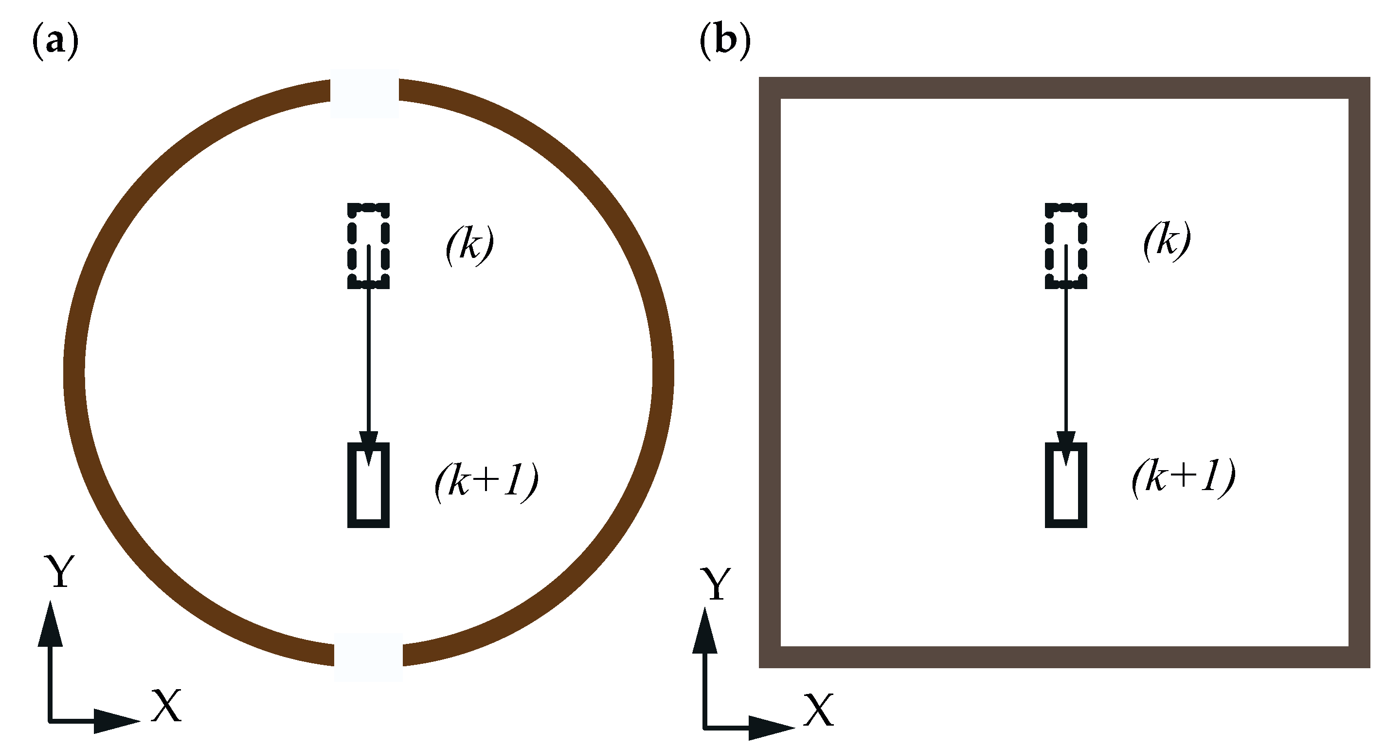
• USV was moving rectilinearly along the N(Y) axis while changing its position step-wise by 1 m within the area whose walls were square or circular in shape.
• The scanning device produced and recorded two sets of environment scans. The first $z{s}_1=\{{s_{\left(k\right)}}_{1,1},$${s_{\left(k\right)}}_{1,2},\dots ,{s_{\left(k\right)}}_{1,900}\}$ at the vehicle’s position at the moment $\left(k\right)$. The second $z{s}_2=\{{s_{(k+1)}}_{2,1},$${s_{(k+1)}}_{2,2},\dots ,$${s_{(k+1)}}_{2,900}\}$ at the vehicle’s position at the moment $(k+1)$.
• The number of points in subsequent scans from the sets $z{s}_1$ and $z{s}_2$ was increased by 1, starting from 100 points (${s_{\left(k\right)}}_{1,1}$, ${s_{(k+1)}}_{2,1}$) and ending after having achieved 1000 points (${s_{\left(k\right)}}_{1,900}$, ${s_{(k+1)}}_{2,900}$). A change in the number of points in the scan was aimed at the simulation, i.e., a change in the angle resolution of the measurement.
• The scan pairs from the sets $z{s}_1$ and $z{s}_2$ (e.g., ${s_{\left(k\right)}}_{1,50}$ and ${s_{(k+1)}}_{2,50}$), corresponding to one another in terms of the number of points, were matched to one another by the standard algorithm, the ICP algorithm—$ICP$, and algorithms based on introduced coefficients—$IC{P}_{ME}$, $IC{P}_{MDE}$, $IC{P}_{VDE}$. Scans from the set $z{s}_1$ were regarded as reference ones.
• Points in the sets $z{s}_1$ and $z{s}_2$ were determined for the walls of figures based on the pairs of measurements of the distances r and the direction $\alpha$ from the vehicles’s position $(x_{\left(k\right)},y_{\left(k\right)})$ at the moment $\left(k\right)$ and $(x_{(k+1)},y_{(k+1)})$ at the moment $(k+1)$. In order to make the simulation more realistic, the corrections $v_r\sim \mathbb{N}(0,{\sigma }_r^2)$, $v_{\alpha }\sim \mathbb{N}(0,{\sigma }_{\alpha }^2)$, where ${\sigma }_r=0,03m$, ${\sigma }_{\alpha }=0,5^{\circ }$ were added to the measurements r and $\alpha$.
• The simulation was carried out 150 times for each of the variants illustrated in Figure 4 for a particular sample size per scan (e.g., 150 times for the scans ${s_{\left(k\right)}}_{1,50}$ and ${s_{(k+1)}}_{2,50}$…, 150 times for ${s_{\left(k\right)}}_{1,51}$ and ${s_{(k+1)}}_{2,51}$, etc.).
• The condition which ended the iterations of ICP algorithm was the assumption that $\Delta <{10}^{-8}\mathrm{m}$ (the equation is presented in line 18 of Algorithm 1).

The simulation result included the parameters of translation and rotation of the model scan to reference scan $\widehat{\mathbf{x}}={\left[\begin{array}{ccc}\Delta {\widehat{x}}_{(k+1)}& \Delta {\widehat{y}}_{(k+1)}& \Delta {\widehat{\theta }}_{(k+1)}\end{array}\right]}^{\mathrm{T}}$. The conducted tests were aimed at determining the elements of descriptive statistics of the distribution from the sample of 150 increments of position coordinates and the estimated rotation ${\widehat{X}}_{(k+1)}(x_k+\Delta {\widehat{x}}_{(k+1)},y_k+\Delta {\widehat{y}}_{(k+1)}),{\theta }_k+\Delta {\widehat{\theta }}_{(k+1)}$ from the reference coordinates and the rotation $X_{(k+1)}(x_{(k+1)},y_{(k+1)}),{\theta }_{(k+1)}$.

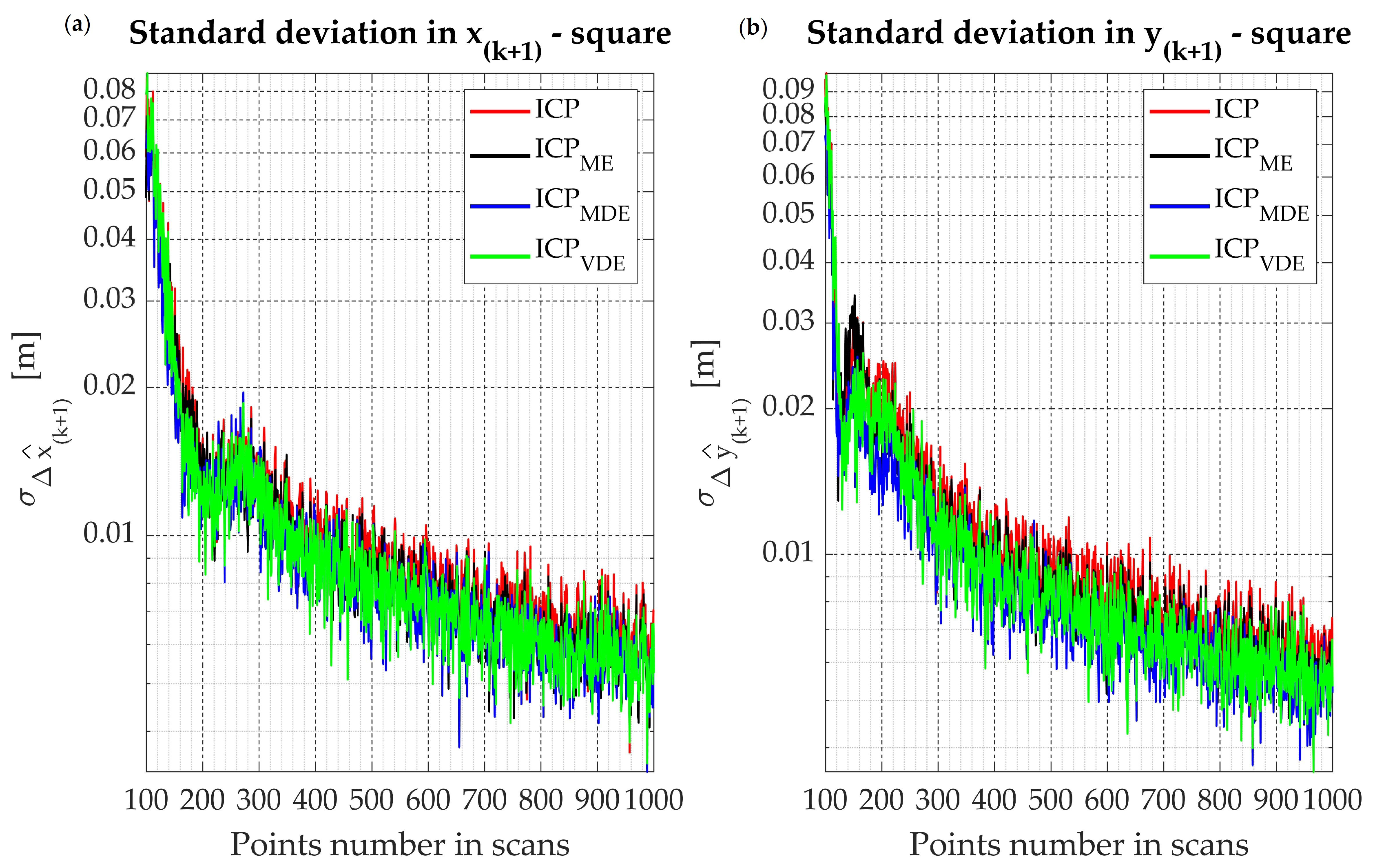
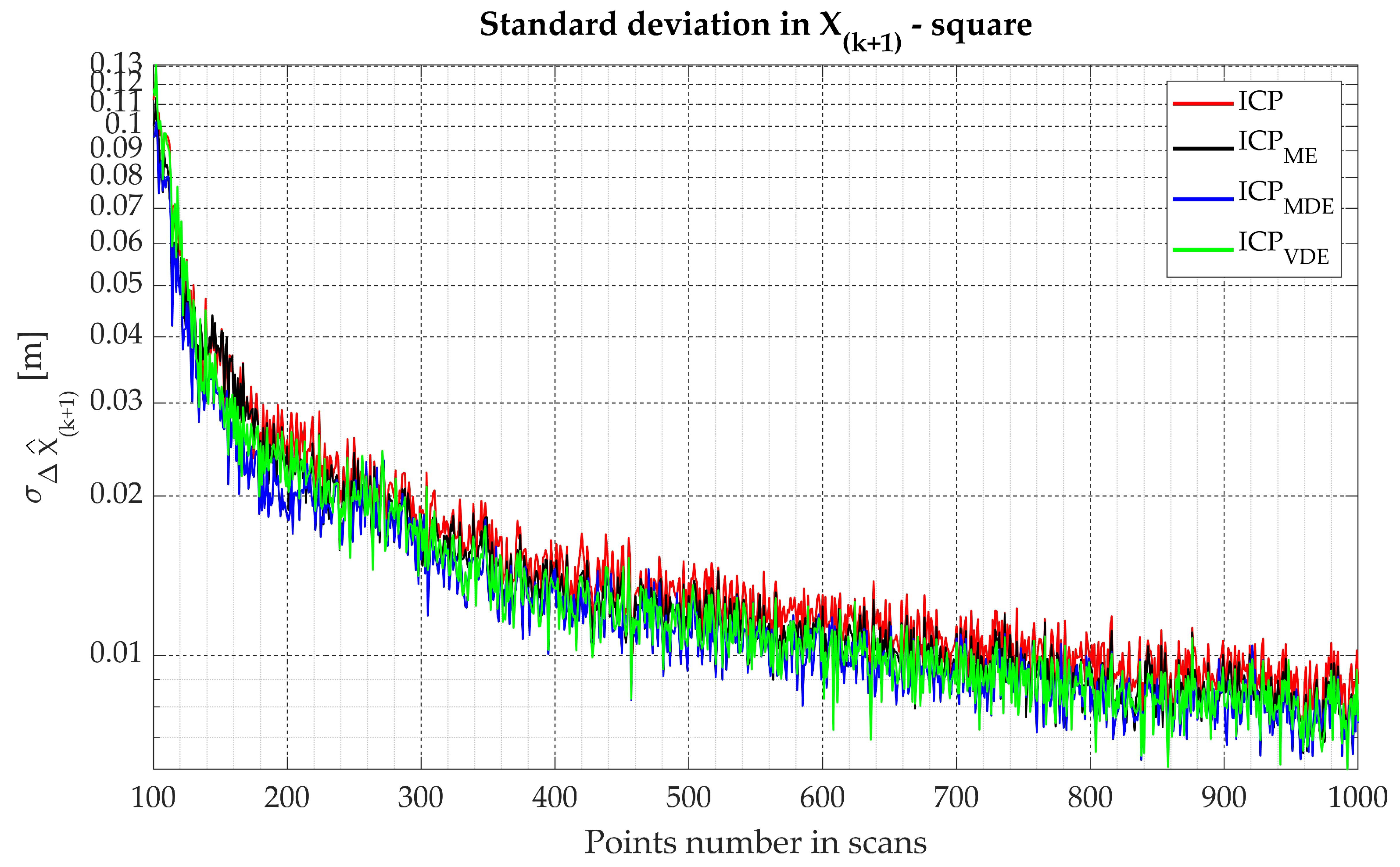
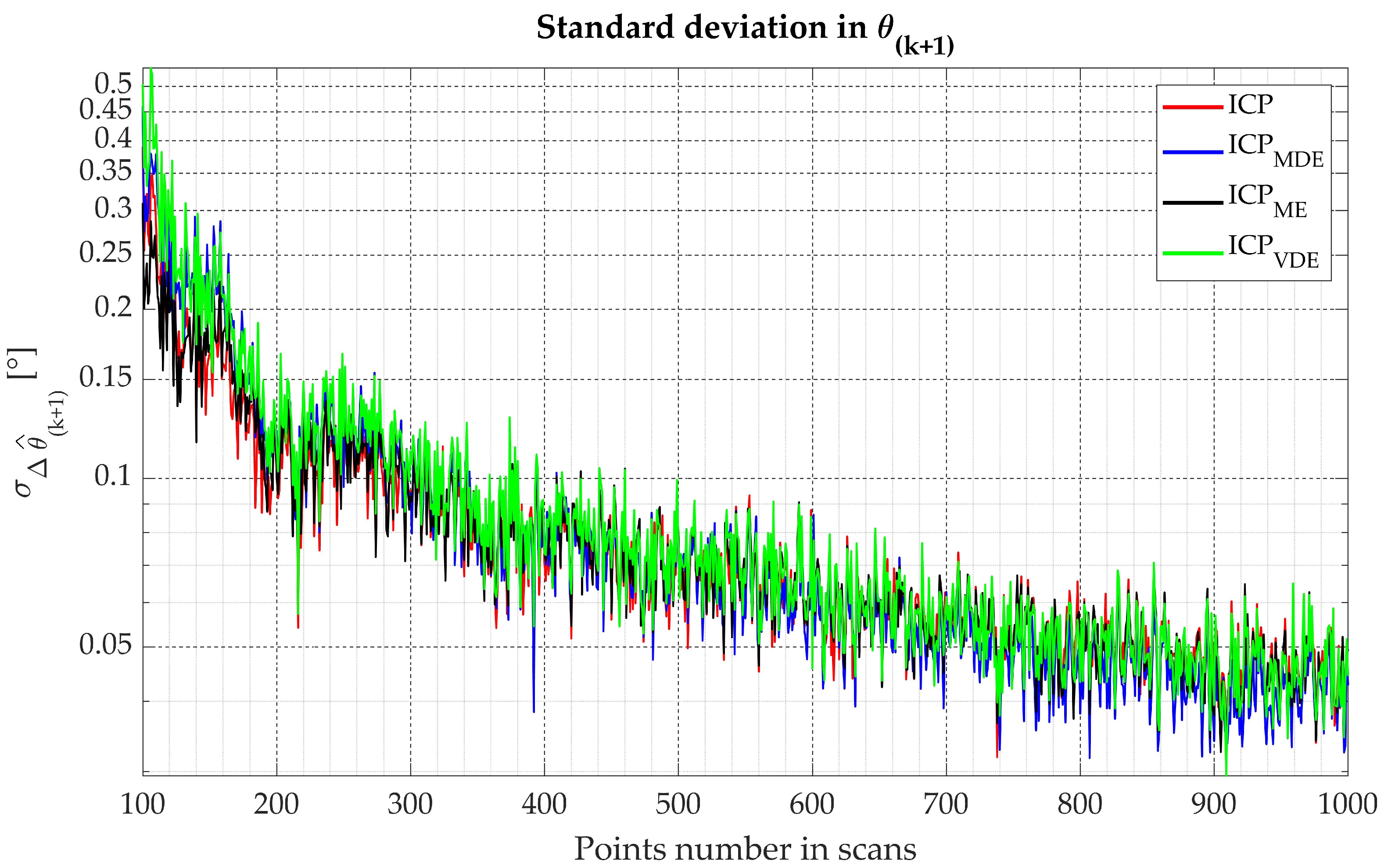
5.1. Results—Translation and Rotation Accuracy in a Square-Shaped Area

For the motion within a square-shaped area, for the initial sample sizes in the sets (for a small number of points), the accuracy of translation on the X-axis is higher than for Y (the values illustrated in Figure 5). However, the initial imbalance is eliminated with an increase in the number of the points concerned. For the entire simulation within the square, the ratio of $\frac{{\sigma }_{{\widehat{y}}_{(k+1)}}}{{\sigma }_{{\widehat{x}}_{(k+1)}}}$ amounts to 0.89–0.93 (depending on the weighting factor type). It should be noted that the motion took place along the Y-axis. Having carried out an accuracy analysis in relation to the Y-axis and the X-axis, the following conclusions can be drawn. $IC{P}_{MDE}$ yielded the most accurate results in $54.4\%$ of cases (along the X-axis), and in $68.5\%$ (along the Y-axis). $IC{P}_{VDE}$ demonstrated the lowest value of standard deviation in $33.0\%$ of cases (along the X-axis), and in $23.3\%$ of cases (along the Y-axis). For the motion within the square-shaped area, $IC{P}_{ME}$ yielded the best accuracy results for $12.6\%$ of cases (along the X-axis), and in $8.2\%$ of cases (along the Y-axis).

The study showed that the most accurate results for the motion within a square-shaped area were demonstrated by the algorithm in the $IC{P}_{MDE}$ version, which was the most accurate in $70\%$ of cases of the increment of ${{\sigma }_{\Delta }}_{{\widehat{X}}_{(k+1)}}$—Figure 6. The algorithm in the $IC{P}_{VDE}$ version proved to be the second in the ranking. The estimated coordinate obtained with its use had the lowest standard deviation values in $27.3\%$ of the cases considered. The last one, $IC{P}_{ME}$, yielded the most accurate position in $2.3\%$ of the cases considered. The standard $ICP$ algorithm demonstrated no lowest value of standard deviation for any of the point number intervals in the scans.

The study showed that the most accurate results for the rotation within a square-shaped area were demonstrated by the algorithm in the $IC{P}_{VDE}$ version, which was the most accurate in $46.8\%$ of cases of the increment of ${{\sigma }_{\Delta }}_{{\widehat{\theta }}_{(k+1)}}$—Figure 7. The standard $ICP$ algorithm proved to be the second in the ranking. The estimated coordinated obtained with its use had the lowest standard deviation values in $20.2\%$ of the cases considered. $IC{P}_{ME}$ yielded the most accurate angle increment in $19.4\%$ of the cases considered, while $IC{P}_{MDE}$ was the most accurate for $13.6\%$ of the cases.

5.2. Results—Translation and Rotation Accuracy in a Circular-Shaped Area

What is noticeable is the greater dispersion of the yielded positions along the motion direction (Figure 8). However, the difference in standard deviation in relation to the axis decreases as the function of the number of points in the scan. Having considered all variants of the number of points in the scans, the ratio $\frac{{\sigma }_{{\widehat{y}}_{(k+1)}}}{{\sigma }_{{\widehat{x}}_{(k+1)}}}$ amounts to 1.04–1.13 (depending on the algorithm variant). This ratio is high for the initial scans from the set (with a small number of points). However, with an increase in the number of points in the scans, it approaches unity. An analysis of the values of the mean error of coordinates ${\widehat{x}}_{(k+1)}$ and ${\widehat{y}}_{(k+1)}$ on the X- and Y-axes leads to conclusions similar to those for the mean error of the position’s coordinates. $IC{P}_{MDE}$ was the most accurate in $84.3\%$ (along the X-axis) and $87.2\%$ (along the Y-axis) of the quantitative variants, while $IC{P}_{VDE}$ was the most accurate in $15.7\%$ of cases (along the X-axis) and $12.8\%$ of cases (along the Y-axis).

The algorithm in two variants, i.e., $IC{P}_{MDE}$ and $IC{P}_{VDE}$, yielded better results in terms of the accuracy of $\Delta {\widehat{X}}_{(k+1)}$ (lower dispersion of the position’s coordinates)—Figure 9. $IC{P}_{MDE}$ was the most accurate in $92.2\%$ of quantitative variants, while $IC{P}_{VDE}$ was the most accurate in $7.8\%$.

The study showed that the most accurate results for the motion within a circular-shaped area were demonstrated by the algorithm in the standard version, which was the most accurate in $47.3\%$ of cases of the increment of ${{\sigma }_{\Delta }}_{{\widehat{\theta }}_{(k+1)}}$—Figure 10. The $IC{P}_{ME}$ algorithm proved to be the second in the ranking. The estimated coordinated obtained with its use had the lowest standard deviation values in $28.9\%$ of the cases considered. $IC{P}_{VDE}$ yielded the most accurate angle increment in $18.9\%$ of the cases considered, while $IC{P}_{MDE}$ was the most accurate in $4.9\%$ of the cases.

5.3. Results—Summary

First of all, it is visible in all graphs (for both, circle and squere-shaped area) [5, 6, 7, 8, 9, 10] that the value of the standard deviation of the estimated increments decreases with an increase in the number of points in the scans. For the actual use of sensors of the LiDAR or RADAR type, neither the same number of points in the neighbouring scans nor the subsequent pairs during the entire measurement can be guaranteed. This is due to measurement equipment interference, the occlusion phenomenon, measurement noise, etc. In view of the above, a tabular (

Table 1. Statistical values characterising the algorithms under study. The values accumulated below were determined for the entire simulation study, without being divided according to the number of points in scans (${{\sigma }_X}_{(k+1)}$ is square root of the sum of squares of standard deviations in two axes).

		Circle			Square
ICP’s Version	${\mathit{ICP}}_{}$	${\mathit{ICP}}_{\mathit{MDE}}$	${\mathit{ICP}}_{\mathit{ME}}$	${\mathit{ICP}}_{\mathit{VDE}}$	$\mathit{ICP}$	${\mathit{ICP}}_{\mathit{MDE}}$	${\mathit{ICP}}_{\mathit{ME}}$	${\mathit{ICP}}_{\mathit{VDE}}$
${{\sigma }_x}_{(k+1)}\left[\mathrm{m}\right]$	0.0074	$0.0059$	0.0073	0.0062	0.0101	$0.0086$	0.0091	0.0102
${{\sigma }_y}_{(k+1)}\left[\mathrm{m}\right]$	0.0080	$0.0058$	0.0077	0.0061	0.0095	$0.0075$	0.0087	0.0093
${{\sigma }_X}_{(k+1)}\left[\mathrm{m}\right]$	0.0111	$0.0084$	0.0107	0.0088	0.0160	$0.0141$	0.0153	0.0150
${{\sigma }_{\theta }}_{(k+1)}{[}^{\circ }]$	0.1213	$0.1112$	0.1126	0.1195	0.1195	0.0836	$0.0795$	0.0889
Proc. time $\left[\mathrm{s}\right]$	0.0423	0.0651	$0.0413$	0.0624	0.0589	0.0923	$0.0564$	0.0876

) summary of results of the entire study (taking into account all the cases considered, i.e., 135,000 scan configurations—150 cases × 900 sample size intervals) was determined, and the data characterising the accuracy of the algorithms in individual variants (presented below) were generated.

5.4. Results—RMS Alignment Error

Researchers into the ICP algorithm focus their particular attention on the RMS alignment error. Studies into this indicator, depending on the algorithm modification, are presented inter alia in [21,40,41]. The mean error of the developed increments of the coordinates and the rotation angle is a different measure in relation to the mean error of environment scans matching using the ICP algorithm. This is a measure that specifies the accuracy of matching of two environment scans as a function of the arithmetic mean of the squares of individual determination deviations (residuals) as

$$RMS=\frac{{\sum }_{i=1}^n\left|\right|{\mathbf{R}}_z{\mathit{p}}_{\mathbf{i}}\left(k\right)+{\mathbf{T}}_z-{{\mathit{p}}_j}_{(k+1)}{\left|\right|}^2}{n}.$$

(19)

As can be noted in Figure 11, the application of weighting factors in the ICP algorithm has a decisive influence on the algorithm’s convergence. The algorithm based on damping based on the mean error in the direction ($IC{P}_{MDE}$) achieves convergence with a smaller number of iterations, i.e., from 5 to 7 iterations depending on the environment. The standard algorithm needs at least three more iterations to achieve the same level of RMS, compared to the $IC{P}_{MDE}$ algorithm. The $IC{P}_{MD}$ algorithm yields the same results in terms of the RMS as the standard algorithm $ICP$.

This part of reserch shows that the use of specific weighting factor reduces not only the number of iterations needed to achieve convergence but also the time required for scan alignment. The results illustrated in Figure 11 were generated for the number of points in the sets $z{s}_1$ and $z{s}_2$ at a level of 500 points.

The results show that despite the long processing time of a single iteration compared to other algorithms, the $IP{C}_{MDE}$ algorithm requires fewer loops and achieves the same convergence level as the other algorithms in a shorter time. The results regarding processing times are given in

Table 2. Time of computation till convergence (RMS on the lavel of $IC{P}_{MDE}$ in 6th iteration for circle and 5th iteration for square).

		Circle			Square
ICP’s Version	${\mathit{ICP}}_{}$	${\mathit{ICP}}_{\mathit{MDE}}$	${\mathit{ICP}}_{\mathit{ME}}$	${\mathit{ICP}}_{\mathit{VDE}}$	$\mathit{ICP}$	${\mathit{ICP}}_{\mathit{MDE}}$	${\mathit{ICP}}_{\mathit{ME}}$	${\mathit{ICP}}_{\mathit{VDE}}$
Proc. time $\left[\mathrm{s}\right]$	0.0223	$0.0199$	$0.0224$	0.0210	0.0254	$0.0212$	$0.0280$	0.0217
No of iterations	8	6	8	7	8	5	8	6
Avg. time of iteration [s]	$0.0027$	0.0033	0.0028	0.0030	$0.0032$	0.0042	0.0035	0.0036

.

6. Conclusions and Further Work

The article presents the results of a simulation study on modified algorithms from the ICP family. Based on an extensive study, it was demonstrated that the proposed modifications based on measurement errors of the mapping sensor contribute considerably to an increase in the accuracy of the obtained translation and rotation angle values. The algorithm, using the proposed modification, also achieved convergence with a smaller number of algorithm iterations. The proposed weighting factors are presented in detail, which may facilitate their further implementation. It should be noted that since the presented methods are based on sensor errors, the error model needs to be perfectly recognised prior to possible use. However, the data obtained in the simulation study indicate that the accuracy of determination of parameters using the $IC{P}_{MDE}$ and $IC{P}_{VDE}$ algorithms is affected by the increased duration of data processing, compared to the standard version. It should be noted, however, that the algorithms were not optimised in terms of speed. The next stage of the study will be the implementation of damping coefficients into the ICP algorithm for three-dimensional space.

References

1. Nieto, J.; Bailey, T.; Nebot, E. Scan-SLAM: Combining EKF-SLAM and Scan Correlation. In Springer Tracts in Advanced Robotics; Springer: Berlin/Heidelberg, Germany, 2006; pp. 167–178. [Google Scholar] [CrossRef]
2. Zhang, J.; Singh, S. LOAM: Lidar Odometry and Mapping in Real-time. In Proceedings of the Robotics: Science and Systems X Conference, Berkeley, CA, USA, 12–16 July 2014. [Google Scholar] [CrossRef]
3. Besl, P.; McKay, N.D. A method for registration of 3-D shapes. IEEE Trans. Pattern Anal. Mach. Intell. 1992, 14, 239–256. [Google Scholar] [CrossRef]
4. Ezra, E.; Sharir, M.; Efrat, A. On the ICP algorithm. In Proceedings of the Twenty-Second Annual Symposium on Computational Geometry—SCG 06; ACM Press: New York, NY, USA, 2006. [Google Scholar] [CrossRef]
5. Baek, S.; Gil, Y. Human Pose Estimation Using Articulated ICP. In Proceedings of the 2019 2nd International Conference on Control and Robot Technology; ACM: New York, NY, USA, 2019. [Google Scholar] [CrossRef]
6. Yang, J.; Li, H.; Campbell, D.; Jia, Y. Go-ICP: A globally optimal solution to 3D ICP point-set registration. IEEE Trans. Pattern Anal. Mach. Intell. 2016, 38, 2241–2254. [Google Scholar] [CrossRef] [PubMed] [Green Version]
7. Diebel, J.; Reutersward, K.; Thrun, S.; Davis, J.; Gupta, R. Simultaneous localization and mapping with active stereo vision. In Proceedings of the 2004 IEEE/RSJ International Conference on Intelligent Robots and Systems (IROS) (IEEE Cat. No.04CH37566), Sendai, Japan, 28 September–2 October 2004; IEEE: New York, NY, USA, 2004. [Google Scholar] [CrossRef]
8. Rowekamper, J.; Sprunk, C.; Tipaldi, G.D.; Stachniss, C.; Pfaff, P.; Burgard, W. On the position accuracy of mobile robot localization based on particle filters combined with scan matching. In Proceedings of the 2012 IEEE/RSJ International Conference on Intelligent Robots and Systems, Vilamoura, Portugal, 7–12 October 2012; IEEE: New York, NY, USA, 2012. [Google Scholar] [CrossRef] [Green Version]
9. Wang, J.; Zhao, M.; Chen, W. MIM_SLAM: A Multi-Level ICP Matching Method for Mobile Robot in Large-Scale and Sparse Scenes. Appl. Sci. 2018, 8, 2432. [Google Scholar] [CrossRef] [Green Version]
10. Jiang, G.; Yin, L.; Liu, G.; Xi, W.; Ou, Y. FFT-Based Scan-Matching for SLAM Applications with Low-Cost Laser Range Finders. Appl. Sci. 2018, 9, 41. [Google Scholar] [CrossRef] [Green Version]
11. Lenac, K.; Cuzzocrea, A.; Mumolo, E. An effective and efficient hybrid scan matching algorithm for mobile object applications. In Proceedings of the Symposium on Applied Computing—SAC 17; ACM Press: New York, NY, USA, 2017. [Google Scholar] [CrossRef]
12. Zhu, Q.; Wu, J.; Hu, H.; Xiao, C.; Chen, W. LIDAR Point Cloud Registration for Sensing and Reconstruction of Unstructured Terrain. Appl. Sci. 2018, 8, 2318. [Google Scholar] [CrossRef] [Green Version]
13. Olson, E.B. Robust and Efficient Robotic Mapping. Ph.D. Thesis, Massachusetts Institute of Technology, Cambridge, MA, USA, 2008. [Google Scholar]
14. Rofer, T. Using histogram correlation to create consistent laser scan maps. In Proceedings of the IEEE/RSJ International Conference on Intelligent Robots and System, Lausanne, Switzerland, 30 September–4 October 2002; IEEE: New York, NY, USA, 2002. [Google Scholar] [CrossRef] [Green Version]
15. Konecny, J.; Prauzek, M.; Kromer, P.; Musilek, P. Novel Point-to-Point Scan Matching Algorithm Based on Cross-Correlation. Mob. Inf. Syst. 2016, 2016, 1–11. [Google Scholar] [CrossRef] [Green Version]
16. Zezhong, X.; Jilin, L.; Zhiyu, X. Scan matching based on CLS relationships. In Proceedings of the IEEE International Conference on Robotics, Intelligent Systems and Signal Processing, Changsha, China, 8–13 October 2003; IEEE: New York, NY, USA, 2003. [Google Scholar] [CrossRef]
17. Zezhong, X.; Jilin, L.; Zhiyu, X. Map building and localization using 2D range scanner. In Proceedings of the 2003 IEEE International Symposium on Computational Intelligence in Robotics and Automation, Kobe, Japan, 16–20 July 2020; IEEE: New York, NY, USA, 2003; Volume 2, pp. 848–853. [Google Scholar]
18. Godin, G.; Rioux, M.; Baribeau, R. Three-dimensional registration using range and intensity information. In Videometrics III; El-Hakim, S.F., Ed.; SPIE: Boston, MA, USA, 1994. [Google Scholar] [CrossRef]
19. Liu, B.; Gao, X.; Liu, H.; Wang, X.; Liang, B. A Fast Weighted Registration Method of 3D Point Cloud Based on Curvature Feature. In Proceedings of the 3rd International Conference on Multimedia and Image Processing—ICMIP 2018; ACM Press: New York, NY, USA, 2018. [Google Scholar] [CrossRef]
20. Wang, R.; Geng, Z. WA-ICP algorithm for tackling ambiguous correspondence. In Proceedings of the 2015 3rd IAPR Asian Conference on Pattern Recognition (ACPR), Kuala Lumpur, Malaysia, 3–6 November 2015; IEEE: New York, NY, USA, 2015. [Google Scholar] [CrossRef]
21. Rusinkiewicz, S.; Levoy, M. Efficient variants of the ICP algorithm. In Proceedings of the Third International Conference on 3-D Digital Imaging and Modeling, Quebec City, QC, Canada, 28 May–1 June 2001; IEEE: New York, NY, USA, 2001. [Google Scholar] [CrossRef] [Green Version]
22. Naus, K.; Marchel, Ł. Use of a Weighted ICP Algorithm to Precisely Determine USV Movement Parameters. Appl. Sci. 2019, 9, 3530. [Google Scholar] [CrossRef] [Green Version]
23. Censi, A. An accurate closed-form estimate of ICPs covariance. In Proceedings of the 2007 IEEE International Conference on Robotics and Automation, Roma, Italy, 10–14 April 2007; IEEE: New York, NY, USA, 2007. [Google Scholar]
24. He, Y.; Liang, B.; Yang, J.; Li, S.; He, J. An Iterative Closest Points Algorithm for Registration of 3D Laser Scanner Point Clouds with Geometric Features. Sensors 2017, 17, 1862. [Google Scholar] [CrossRef] [PubMed] [Green Version]
25. Bengtsson, O.; Albert-Jan, B. Robot localization based on scan-matching estimating the covariance matrix for the IDC algorithm. Robot. Auton. Syst. 2003, 44, 29–40. [Google Scholar] [CrossRef]
26. Marden, S.; Guivant, J. Improving the Performance of ICP for Real-Time Applications using an Approximate Nearest Neighbour Search. In Proceedings of the Australasian Conference on Robotics and Automation, Wellington, New Zealand, 3–5 December 2012; pp. 3–5. [Google Scholar]
27. Leal, N.; Zurek, E.; Leal, E. Non-Local SVD Denoising of MRI Based on Sparse Representations. Sensors 2020, 20, 1536. [Google Scholar] [CrossRef] [PubMed] [Green Version]
28. Pfister, S.; Kriechbaum, K.; Roumeliotis, S.; Burdick, J. Weighted range sensor matching algorithms for mobile robot displacement estimation. In Proceedings of the 2002 IEEE International Conference on Robotics and Automation, Washington, DC, USA, 11–15 May 2002; IEEE: New York, NY, USA, 2002. [Google Scholar] [CrossRef] [Green Version]
29. Barczyk, M.; Bonnabel, S. Towards realistic covariance estimation of ICP-based Kinect V1 scan matching: The 1D case. In Proceedings of the 2017 American Control Conference (ACC), Seattle, WA, USA, 24–26 May 2017; IEEE: New York, NY, USA, 2017. [Google Scholar] [CrossRef] [Green Version]
30. Brossard, M.; Bonnabel, S.; Barrau, A. A New Approach to 3D ICP Covariance Estimation. IEEE Robot. Autom. Lett. 2020, 5, 744–751. [Google Scholar] [CrossRef] [Green Version]
31. Pomerleau, F.; Breitenmoser, A.; Liu, M.; Colas, F.; Siegwart, R. Noise characterization of depth sensors for surface inspections. In Proceedings of the 2012 2nd International Conference on Applied Robotics for the Power Industry (CARPI), Zurich, Switzerland, 11–13 September 2012; IEEE: New York, NY, USA, 2012. [Google Scholar] [CrossRef] [Green Version]
32. Wang, Z.; Liu, Y.; Liao, Q.; Ye, H.; Liu, M.; Wang, L. Characterization of a RS-LiDAR for 3D Perception. arXiv 2018, arXiv:1709.07641v1. [Google Scholar]
33. Laconte, J.; Deschenes, S.P.; Labussiere, M.; Pomerleau, F. Lidar Measurement Bias Estimation via Return Waveform Modelling in a Context of 3D Mapping. In Proceedings of the 2019 International Conference on Robotics and Automation (ICRA), Montreal, QC, Canada, 20–24 May 2019; IEEE: New York, NY, USA, 2019. [Google Scholar] [CrossRef] [Green Version]
34. Deschaud, J.E. IMLS-SLAM: Scan-to-Model Matching Based on 3D Data. In Proceedings of the 2018 IEEE International Conference on Robotics and Automation (ICRA), Brisbane, QLD, Australia, 21–25 May 2018; IEEE: New York, NY, USA, 2018. [Google Scholar] [CrossRef] [Green Version]
35. Landry, D.; Pomerleau, F.; Giguère, P. CELLO-3D: Estimating the Covariance of ICP in the Real World. arXiv 2019, arXiv:1810.01470v1. [Google Scholar]
36. Iversen, T.M.; Buch, A.G.; Kraft, D. Prediction of ICP pose uncertainties using Monte Carlo simulation with synthetic depth images. In Proceedings of the 2017 IEEE/RSJ International Conference on Intelligent Robots and Systems (IROS), Vancouver, BC, Canada, 24–28 September 2017; IEEE: New York, NY, USA, 2017. [Google Scholar] [CrossRef]
37. Pomerleau, F.; Colas, F.; Siegwart, R. A Review of Point Cloud Registration Algorithms for Mobile Robotics. Found. Trends Robot. 2015, 4, 1–104. [Google Scholar] [CrossRef] [Green Version]
38. Naus, K.; Nowak, A. The Positioning Accuracy of BAUV Using Fusion of Data from USBL System and Movement Parameters Measurements. Sensors 2016, 16, 1279. [Google Scholar] [CrossRef] [Green Version]
39. Marchel, Ł.; Naus, k.; Specht, M. Optimisation of the Position of Navigational Aids for the Purposes of SLAM technology for Accuracy of Vessel Positioning. J. Navig. 2019, 73, 282–295. [Google Scholar] [CrossRef] [Green Version]
40. Du, S.; Xu, Y.; Wan, T.; Hu, H.; Zhang, S.; Xu, G.; Zhang, X. Robust iterative closest point algorithm based on global reference point for rotation invariant registration. PLoS ONE 2017, 12, e0188039. [Google Scholar] [CrossRef] [PubMed] [Green Version]
41. Tazir, M.; Gokhool, T.; Checchin, P.; Malaterre, L.; Trassoudaine, L. CICP: Cluster Iterative Closest Point for Sparse-Dense Point Cloud Registration. Robot. Auton. Syst. 2018, 108, 66–86. [Google Scholar] [CrossRef] [Green Version]
Figure 1. Scans of a room: (a) prior to matching; (b) following matching by the Iterative Closest Point (ICP) algorithm.
Energies 13 05939 g001
Figure 2. The principle of measurement by a mapping sensor with the positional line errors taken into account.
Energies 13 05939 g002
Figure 3. Graphical representation of the: (a) mean error; (b) vector error in the direction, and (c) mean error in the direction.
Energies 13 05939 g003
Figure 4. Simulation tests (a) motion within a circle with a radius of 15 m; (b) motion within a square with a side length of 30 m.
Energies 13 05939 g004
Figure 5. Standard deviations of the increments of coordinates (a) along the OX axis; (b) along the OY axis.
Energies 13 05939 g005
Figure 6. The root of the sum of deviation squares along the OX and OY axes, the mean error of the coordinates X ( k + 1 ) for the motion within a square.
Energies 13 05939 g006
Figure 7. Standard deviation of the determination of the rotation angle increment Δ θ ( k + 1 ) within a square.
Energies 13 05939 g007
Figure 8. Standard deviations of the increments of coordinates (a) along the OX axis; (b) along the OY axis.
Energies 13 05939 g008
Figure 9. The root of the sum of deviation squares along the OX and OY axes, the mean error of the coordinates X ( k + 1 ) for the motion within a circle.
Energies 13 05939 g009
Figure 10. Standard deviation of the determination of the rotation angle increment Δ θ ( k + 1 ) within a circle.
Energies 13 05939 g010
Figure 11. The mean square error of the matching of scans s ( k ) to s ( k + 1 ) as a function of the number of iterations for the sample size of 500 points in the scans: (a) for the motion within a circular-shaped area (b) for the motion within a square-shaped area.
Energies 13 05939 g011