Deep Reinforcement Learning Control of Cylinder Flow Using Rotary Oscillations at Low Reynolds Number

Abstract

We apply deep reinforcement learning to active closed-loop control of a two-dimensional flow over a cylinder oscillating around its axis with a time-dependent angular velocity representing the only control parameter. Experimenting with the angular velocity, the neural network is able to devise a control strategy based on low frequency harmonic oscillations with some additional modulations to stabilize the Kármán vortex street at a low Reynolds number $Re=100$. We examine the convergence issue for two reward functions showing that later epoch number does not always guarantee a better result. The performance of the controller provide the drag reduction of 14% or 16% depending on the employed reward function. The additional efforts are very low as the maximum amplitude of the angular velocity is equal to $8\%$ of the incoming flow in the first case while the latter reward function returns an impressive $0.8\%$ rotation amplitude which is comparable with the state-of-the-art adjoint optimization results. A detailed comparison with a flow controlled by harmonic oscillations with fixed amplitude and frequency is presented, highlighting the benefits of a feedback loop.

1. Introduction

A well-known Kármán vortex street is typically formed in the wake of the flow over a bluff body exerting an oscillating value of the force [1]. This unsteadiness may cause structural damages due to the coupling of the body vibrations and pressure fluctuations of the fluid. Over time, many flow control strategies have been proposed to influence and suppress these unwanted dynamical features [2]. The overall classification includes passive and active methods due to the possible energetic input to the flow [3]. Active methods represent open- and closed-loop control, depending on the presence of a feedback from sensors to actuators with a further update of a control signal. An appealing way to design new closed-loop control strategies is to rely on the so-called data-driven and learning-based methods, which lately receive well-deserved attention [4].

In fluid dynamics, machine learning techniques have been fruitfully applied to the issue of the turbulence closure modelling within Large-eddy simulations and Reynolds-averaged Navier–Stokes equations [5], estimating and reconstructing flow fields [6], recovering dynamical features [7] and control [8]. In particular, closed-loop flow control extensively benefits from the application of genetic algorithms to canonical turbulent flows, such as mixing layers, jets and wakes [9,10,11,12,13,14,15,16,17,18,19]. Contrary to the typical gradient-based optimization techniques, these methods introduce a population of the control laws which are selected step-by-step according to the target objective function. Even more promising is a combination of multilayer (deep) neural networks combined with the reinforcement learning (RL) strategy [20] resulting in a deep reinforcement learning (DRL) paradigm succeeding in a large number of multidisciplinary problems [21] as well as fluid dynamics in particular [22]. RL represents a self-learning strategy introducing an agent who interacts with the environment through particular actions in order to get a maximum reward. Recent examples mainly consider the manipulation of the flow over a cylinder using multiple synthetic jets and numerical simulations at low Reynolds numbers delivering robust DRL-based control strategies [23,24,25,26,27,28] as well as other applications [29,30,31,32].

In this work, we study a closed-loop control strategy for the flow over a cylinder rotating around its axis with the time-dependent angular velocity being the only control parameter. The direct numerical simulations (DNS) of the Navier–Stokes equations are employed coupled with the DRL method, which relies on the proximal policy optimization algorithm [33] maximizing the expected reward. The reward value is based on the lift and drag forces acting on the cylinder with the neural network employing the information on the pressure field in the wake region. The particular focus of the work is on the deviation of the control signal from the intuitive one typically considered as a harmonic oscillation.

The control method based on sinusoidal wall oscillations around the axis of the cylinder is known to dramatically suppress the drag coefficient up to 85% for a certain parameters of the amplitude and frequency for $Re=1.5\times {10}^4$ [34]. This experimental result has been qualitatively confirmed by a series of numerical simulations extending the study to even higher $Re=1.4\times {10}^5$ demonstrating that high-frequency and rather high-amplitude rotary oscillations lead to even larger decrease of the drag [35,36,37,38,39]. These experiments also showed that the method is energetically efficient only for high Reynolds numbers. However, at low Reynolds numbers, the drag reduction is not that impressive with a decrease between 30% and 60% [40,41,42,43,44,45]. One way to improve this performance and neutralize the effect of the fluid viscosity is to reduce the amplitude of oscillations also avoiding high-frequency rotary motion. This fact indicates that the harmonic control signal at low $Re$ is far from optimal. To stabilize the vortex shedding, a closed-loop strategy has to be employed rather than a straightforward destruction of the wake region by a high-frequency harmonic motion. A feedback optimization has already been used for low Reynolds numbers, although constraining the control to sinusoidal-based forcing and its basic extensions [41,45,46]. The optimal control approach relying on the adjoint optimization and control law of the free waveform provided a reduction of up to 15% for $Re=150$, obtaining the required low amplitude rotary motion [43]. The results depend on the time horizon of the optimization procedure. Recently, it has been shown that a significant increase of the time horizon leads to the drag reduction of 19% for $Re=100$ together with a low-amplitude control law. Thus, the results of optimal control theory may serve as a verification point for the fully data-driven DRL method with a reduced complexity of implementation.

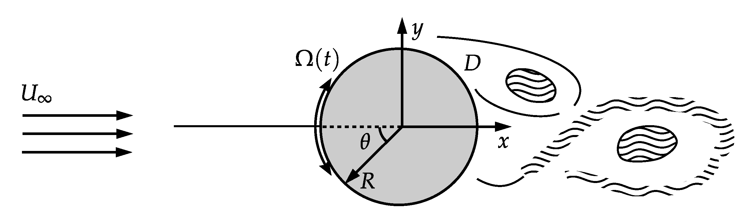
2. Problem Formulation and Computational Details

We consider a cylinder of the diameter D in a fluid cross-flow with a uniform incoming velocity $U_{\infty }$ (see Figure 1). The considered Reynolds number $Re=U_{\infty }D/\nu =100$ representing a laminar flow regime with a Kármán vortex shedding, where $\nu$ is the kinematic viscosity. The applied control strategy is based on the rotation of the cylinder around its axis with the wall velocity $U_w\left(t\right)=U_{\infty }\Omega \left(t\right)$. The primary goal is to find the optimal signal $\Omega \left(t\right)$ to influence drag and lift coefficients:

$$C_D=\frac{2F_x}{{\displaystyle \rho U_{\infty }^2}},C_L=\frac{2F_y}{{\displaystyle \rho U_{\infty }^2}},$$

(1)

where $F_x$ and $F_y$ are the drag and lift forces acting on the cylinder per unit length and $\rho$ is the fluid density.

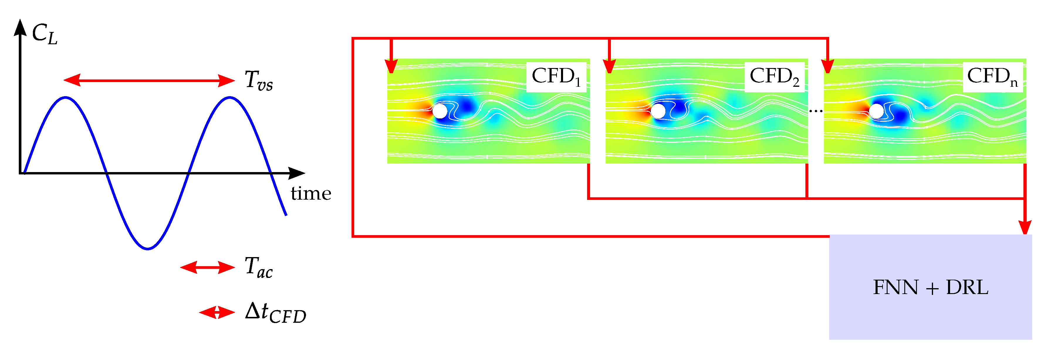
2.1. Flow Computations

To describe the flow field, we solve the non-dimensional incompressible Navier–Stokes equations:

$$\frac{\partial u_i}{\partial t}+u_j\frac{\partial u_i}{\partial x_j}=-\frac{\partial p}{\partial x_i}+\frac{1}{Re}\frac{{\partial }^2{u}_i}{\partial x_j^2},\frac{\partial u_j}{\partial x_j}=0,$$

(2)

where $u_i$ and p are the velocity components and pressure field and all quantities are non-dimensionalized using $U_{\infty }$ and D. We employ direct numerical simulations in a two-dimensional setup with the coordinate system located in the center of the cylinder and x, y representing the streamwise and vertical coordinates, respectively. The computations are performed using an open source unstructured finite-volume code T-Flows below referred to as the CFD solver [47,48]. The code features second-order accurate discretization in space and time. The SIMPLE algorithm is used to couple velocity and pressure fields. The dimensions of the computational domain representing a rectangle are $L_x\times L_y=30D\times 20D$ in the streamwise and vertical directions with the center of the cylinder placed $10D$ from the inlet boundary. The slip condition is set at the top and bottom boundaries and convective outflow condition is prescribed at the outlet, while control law representing the tangential velocity of the cylinder wall is described below. The mesh contains $15,140$ hexahedral cells and the computational timestep is $\Delta t_{CFD}={10}^{-2}$. We validate the simulations of the stationary cylinder case. The typical quantities of interest are the time-averaged drag coefficient ${\overline{C}}_D=1.33$ and vortex shedding frequency $f_{vs}=0.17$, which are in excellent agreement with available results [1].

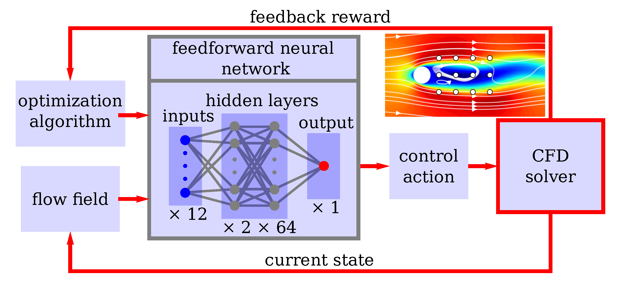
2.2. Machine-Learning Architecture, Feedback Loop and Parallelization

Below, we describe a set of algorithms employed to obtain the angular velocity signal $\Omega \left(t\right)$ with the closed-loop controller synthesized by training a fully connected neural network (FNN). The optimal control strategy evaluation relies on the reinforcement learning (RL) approach [20] and a policy gradient (PG) algorithm [33] with a maximization of a defined reward function. A schematic view of optimization of the feedback control system is shown in Figure 2. In RL, the environment representing the CFD solver interacts with the agent which is the FNN controller in our case. The agent takes a new action based on the current state of the environment representing the data from $4\times 3$ array of pressure sensors placed in the near wake beside the cylinder (see ‘inputs’ and the flow schematics in Figure 2). The FNN has two hidden layers with 64 neurons each and a single output for the mean of the policy PDF of the cylinder angular velocity during evaluation of the controller. The training employed two networks of the similar structure for policy and value prediction including a trainable dispersion coefficient of the policy PDF for a smooth transition from exploration to exploitation of the learned policy. The number of neurons was determined experimentally observing the learning speed and the mean reward after convergence with a fixed number of inputs and the reward function. The neurons in the hidden layers used the sigmoidal activation function while the activation of the output neuron was linear. The action defined the next value of $\Omega$ which was put forward to the CFD solver with a specific relaxation procedure in time. The action time step $T_{ac}$ was set small enough compared to the characteristic time scale $T_{vs}=1/f_{vs}$ of the vortex shedding according to recommendations [24] (see Figure 3 for the hierarchy of timescales). We employed the value $T_{ac}\approx 0.05T_{vs}$ with $T_{ac}=30\Delta t_{CFD}=0.3$. After receiving a new target value of $\Omega$, the angular velocity of the cylinder was updated from the old value to a new target one linearly in time within the whole interval $T_{ac}$. We performed additional tests with the exponential relaxation scheme [24] as well as step-like change of $\Omega$; however, a better behavior of the linear one for a test harmonic control law was observed.

The parallelization strategy is twofold and represents a cornerstone of this research. The CFD code employs a standard MPI-based decomposition of the computational domain with each subdomain treated by a separate computational core. However, with the present low number of cells the speed-up is limited by the number around 10 cores due to the necessary frequent data exchange between neighboring domains sharing common cell faces. For RL algorithms, one needs a sufficient number of actions or control steps for the optimization scheme to succeed. Recently, a successful multi-environment approach [25] has been proposed where multiple independent CFD runs feed the data to one optimization algorithm (see Figure 3). Following this approach, we used three independent CFD runs in parallel with a typical wall time for training a controller using a blade server with two CPUs Intel(R) Xeon(R) CPU E5-2695 v2 @ 2.40GHz with 24 cores in total taking around three days with full CPU utilization. This parallelization was implemented through a vectorized environment feature provided in the OpenAI Baselines code [49] used in this study. As a parameter for the control optimization algorithm, we chose the learning rate constant of the value $3\times {10}^{-4}$, clip parameter $\epsilon =0.2$, GAE parameters with discount rate $\gamma =0.99$ and $\lambda =0.95$, value coefficient $c_1=0.5$ and entropy coefficient $c_2=0.01$ [33]. The instantaneous reward value was parameterized in the following form:

$$r=R_1-({\langle C_D\rangle }_{ac}+R_2|{\langle C_L\rangle }_{ac}\left|\right),$$

(3)

where the drag and lift coefficients were averaged over the action time step. For convenience, the constant $R_1$ was chosen so that the reward values per action were close to zero. The non-zero constant $C_2$ is expected to constrain the non-zero time-averaged lift, leading to the asymmetric flow regimes. With $R_2=0$, in the long run, the control law tended to return a rotating regime. We chose the final value as $R_1=3$ and tried two cases with $R_2=0.1$ (Case 1) and $R_2=0.2$ (Case 2) [24]. The code with the DRL agent adapted for the CFD solver and the corresponding configuration can be found in a public Github repository [50].

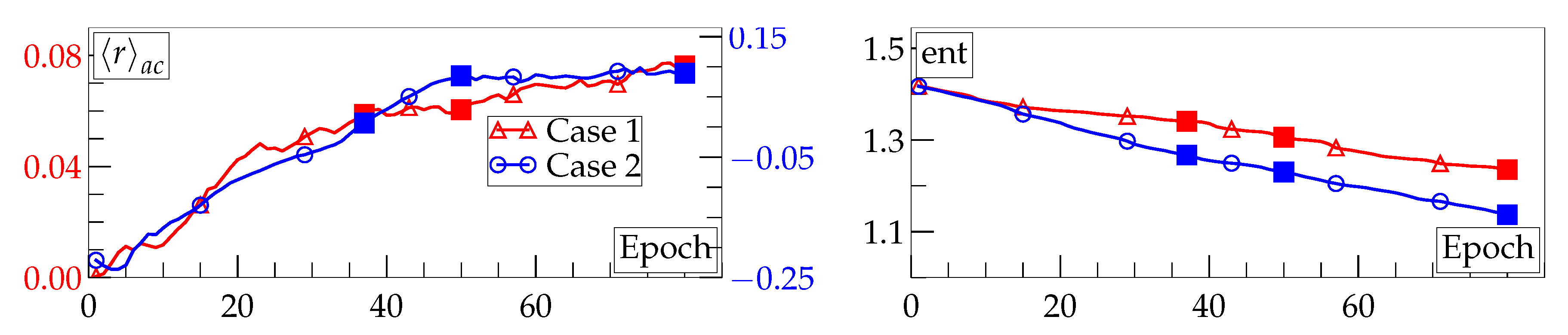
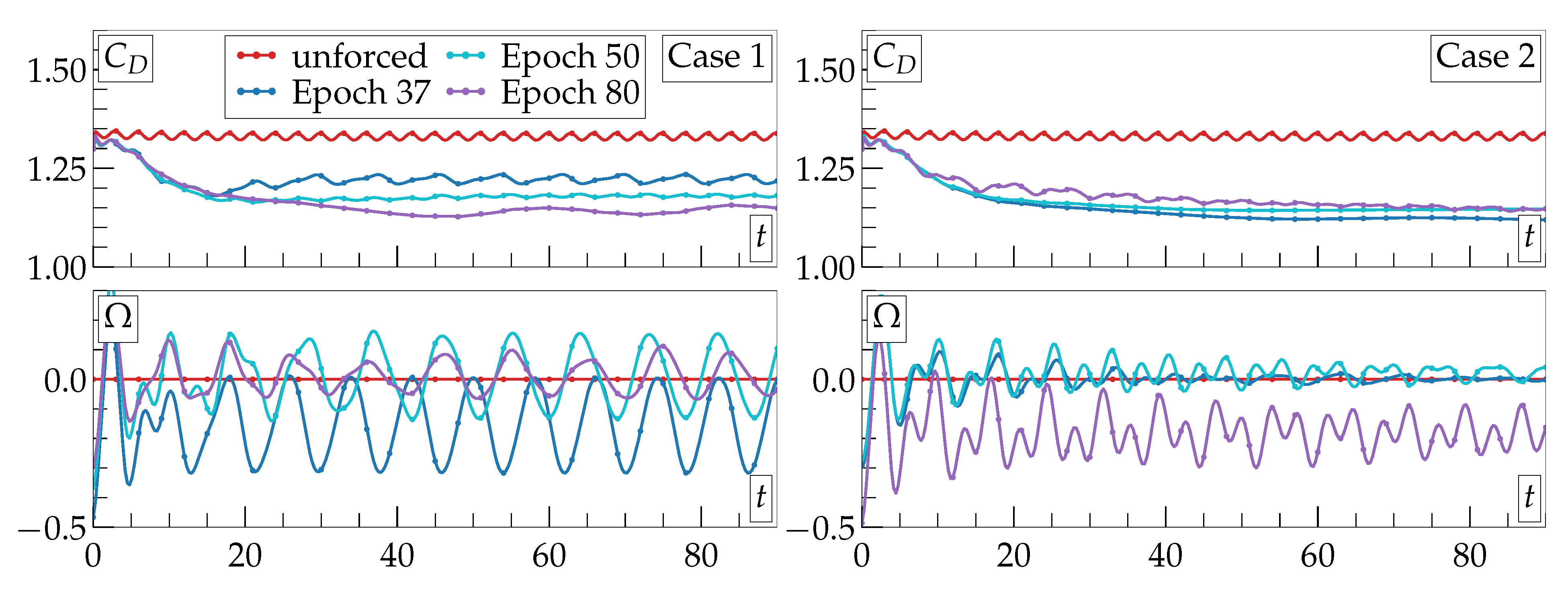
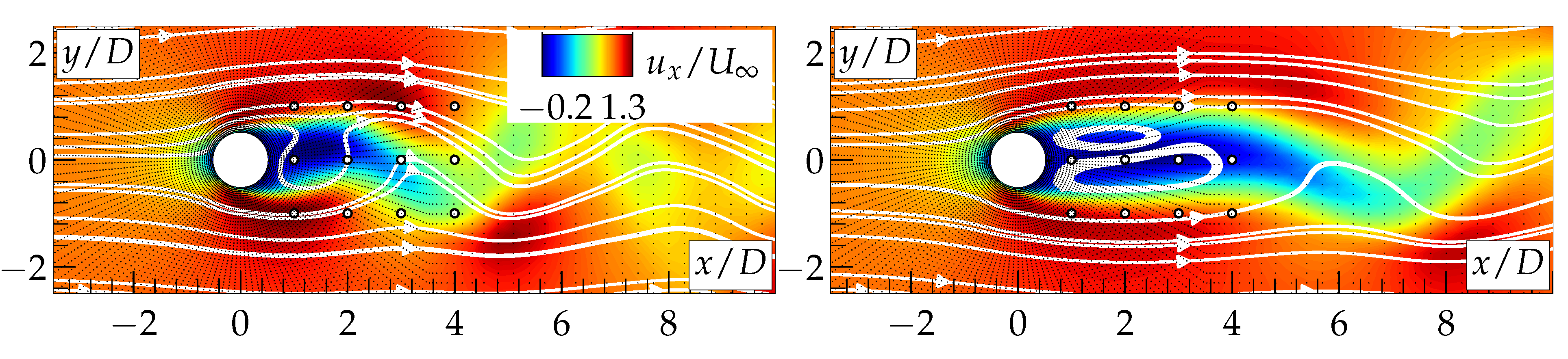
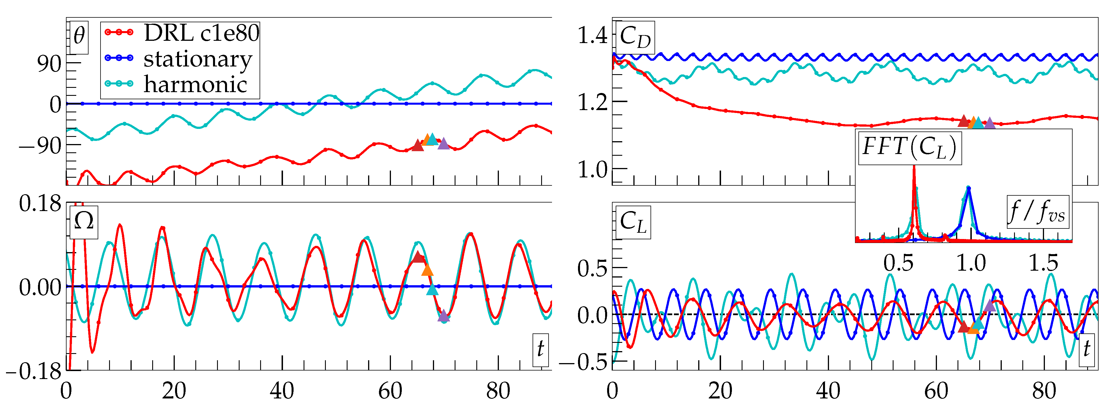
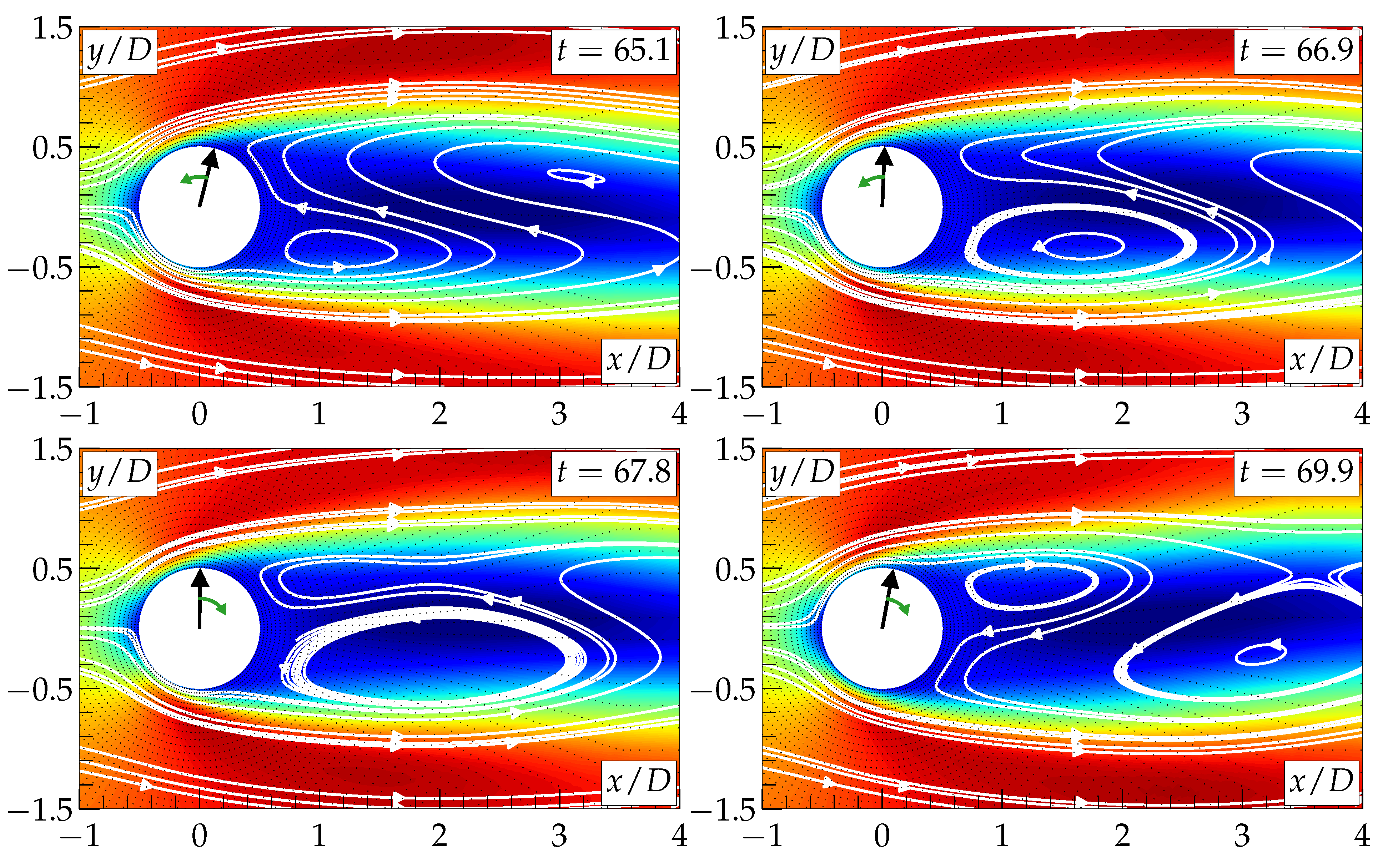
3. Results and Discussion

We performed the training process for 80 epochs to test the convergence issue where the epoch corresponds to the interval between control actions resulting in the overall time interval of nearly 40,000 time units in terms of $D/U_{\infty }$. Figure 4 shows a typical evolution of the reward value averaged over the action time step ${\langle r\rangle }_{ac}$ reaching the saturation after around 50 epochs for Case 2 while still growing for Case 1. The entropy function is expected to characterize the convergence of the training process and decreases monotonically for both cases, indicating that the controller behaves more deterministic and less exploratory with increasing the number of epoch [33].

However, as for the on-policy algorithm a new training set is generated before each policy update using a recently obtained result, stabilization of the algorithm remains an issue [20]. Below, we demonstrate this inherent instability due to a small change of a reward function altering the convergence and leading to a situation with a better policy obtained in the middle of the training process. After accomplishing the training process, we evaluated the performance of the neural controllers.

Table 1. Characteristics of several flow regimes corresponding to the number of epoch during the training process, as depicted in Figure 4 by square points.

	c1e37	c1e50	c1e80	c2e37	c2e50	c2e80
$\Delta {\overline{C}}_D$ (%)	8.1	11.3	13.9	16.1	13.7	14.7
$\Delta (\mathrm{rms}{C}_L$) (%)	−50.5	−21.8	29.6	92.8	86.1	76.8
$\Delta \Omega /2$	0.158	0.139	0.082	0.008	0.031	0.126
$\alpha$ (${}^{\circ }$)	−17.1	1.37	1.39	0.178	2.58	−20.6

and Figure 5 summarize the characteristics of the flow regimes with the applied DRL-based control scheme corresponding to the number of epochs during the training process depicted in Figure 4 by square points below referred to as ‘cXeY’, where ‘X’ stands for the case number (1 or 2) while ‘Y’ corresponds to the epoch number (37, 50 or 80). We address the issue of the drag reduction as well as the change of the root-mean-square of the lift coefficient in comparison with the stationary cylinder flow.

Note an opposite behavior of $C_D$ signal and other characteristics with the increase of the epoch number for Cases 1 and 2. While c1e80 features a decrease of ${\overline{C}}_D$ with $\Delta {\overline{C}}_D=13.9\%$ compared to stationary cylinder regime and outperforms earlier epochs, c2e37 appears to be more optimal compared to later epochs with $\Delta {\overline{C}}_D=16.1\%$. We introduce $\Delta \Omega ={\Omega }_{max}-{\Omega }_{min}$ to evaluate tangential velocity amplitude with the value $\Delta \Omega$ being averaged over a number of local maximum ${\Omega }_{max}$ and minimum ${\Omega }_{min}$ values, respectively. The same cases, c1e80 and c2e37, return the lowest amplitude within each run with $\Delta \Omega /2=8.2\%$ and impressive $0.8\%$ of $U_{\infty }$, respectively. Coming back to the reward value parameterization as in Equation (3), we mention the possible asymmetric flow behavior due to DRL control. Indeed, Cases 1 and 2 (see Table 1) for different epoch numbers recover strategies displaying constant rotation of a fixed point on the surface of the cylinder $\theta \left(t\right)$ as $\alpha t$ combined with oscillatory perturbation ${\theta }^{\prime }\left(t\right)$, i.e., $\theta =\alpha t+{\theta }^{\prime }$ with the angle expressed in degrees, even with $C_L$ being present in the reward expression. Although $\alpha$ is nonzero for most of the regimes, it is relatively low for two out of three cases for each run with the maximum value $\alpha =-{17.1}^{\circ }$ and $-{20.6}^{\circ }$ for c1e37 and c2e80, respectively. Below, we proceed with the analysis of c1e80 as the case where the outcome delivers an appealing slightly modulated harmonic control strategy while better performing c2e37 represents a mixture of a few Fourier modes with close frequency values and may be not very intuitive as an example.

Figure 6 shows the instantaneous streamwise velocity field around the cylinder for the case without control and corresponding to the DRL-based scheme for c1e80 case after a new steady state is reached with its evolution shown in Figure 7. As a result, the flow stabilizes close to the cylinder with a small rotational input trying to balance this inherent instability. The length of the recirculation bubble becomes larger with the local pressure minimum moving further downstream. This leads to a smaller pressure difference between the front and rear of the cylinder with a final decrease of $C_D$. Figure 7 shows the evolution of several characteristics such as the angle $\theta$, angular velocity $\Omega$ and drag and lift coefficients $C_D$ and $C_L$ for different flow regimes. The case of a stationary cylinder is demonstrated as a reference one with $\theta =\Omega =0$. The drag coefficient exhibits sinusoidal behavior with a frequency $2f_{vs}$ around a time-averaged value ${\overline{C}}_D=1.33$ while $C_L$ fluctuates with a natural frequency $f_{vs}=0.17$, reflecting the vortex shedding process, as mentioned above. The application of the DRL-scheme corresponding to c1e80 for control leads to a transient period of about 20 time units, resulting in a modulated harmonic signal of the angular velocity $\Omega$. However, the angle $\theta$ also evolves harmonically in time with a linear trend of a relatively small slope $\alpha ={1.39}^{\circ }$ (see Table 1), corresponding to around ${14}^{\circ }$ rotation within the period $T_1=1/f_1\approx 10$ where $f_1\approx 0.6f_{vs}$ represents the main peak of the Fourier spectrum of the $C_L$ signal. Note also secondary peaks at higher and lower frequencies giving room for modulations of $\Omega$ (see the peaks at $\approx 0.2$, $0.4$ and $0.8f_{vs}$). These modulations turn out to be essential for a drag reduction which is demonstrated in a straightforward manner. We apply a modulated harmonic forcing to the cylinder with $\Omega ={\Omega }_0[sin(2\pi f_{1}t+{\phi }_1)+0.15][1+0.1sin(2\pi f_{2}t+{\phi }_2)]$ where ${\Omega }_0=0.09$, $f_1=0.61f_{vs}$, $f_2=0.22f_{vs}$ well approximates the signal from a DRL-scheme. The outcome of this control strategy is a slight decrease of ${\overline{C}}_D=1.28$ compared to the stationary case and is far from a DRL-scheme. Thus, the feedback loop is indeed gives a benefit for active flow control correctly responding to the instantaneous phase of the vortex shedding process by tuning the angular velocity of the cylinder to stabilize the wake and decrease the drag.

As mentioned above, the DRL-scheme stabilizes the recirculation bubble suppressing the formation of the Kármán vortex street and leading to the elongated bubble behind the bluff body with the reduced value of $C_D$. The mechanism behind the curtain represents the phasor control (see [51] for applications to wake flows), when the appropriate value of almost harmonic variation of angular velocity of the cylinder acts on the near-wall fluid. To get some additional insight into the control routine, Figure 8 shows the instantaneous streamwise velocity field corresponding to four time instants highlighted with triangular symbols in Figure 7 spanning half of the oscillation period of $\Omega$.

At $t=65.1$, the rotation amplitude reaches its local maximum while rotating counterclockwise (see Figure 7). Previous time history shows that $C_D$ and $C_L$ are monotonically decreasing with time and reward function increases. DRL-scheme continues the counterclockwise rotation while also stimulating the growth of the attached eddy in the lower side of the cylinder. Reaching a certain size the eddy and its asymmetric location lead to the increase of $|C_L|$ as for $t=67.8$, which negatively affects the reward function r. To counteract this trend, DRL-scheme switches the rotation direction producing new recirculation zone on the upper side of the cylinder at $t=69.9$, leading to a more symmetric bubble reversing the growth of $C_L$.

4. Conclusions

We applied deep reinforcement learning to active closed-loop control of a two-dimensional flow over a cylinder oscillating around its axis with a time-dependent angular velocity representing the only control parameter. Probing different values of the angular velocity, the neural network was able to create a control strategy based on low frequency harmonic oscillations with some additional modulations to stabilize the Kármán vortex street at a low Reynolds number $Re=100$. We examined the convergence issue for two reward functions showing that later epoch number does not always guarantee a better result. The performance of the controller provide the drag reduction of 14% or 16% depending on the employed reward function comparable with a state-of-the-art control theory optimization routines based on adjoint methods [52]. The additional input of energy to rotate the cylinder was very low as the maximum amplitude of the angular velocity was equal to $8\%$ of the incoming flow in the first case while the latter reward function returned an impressive $0.8\%$ rotation amplitude. A detailed comparison with a flow controlled by harmonic oscillations with one frequency and a fixed amplitude is presented, highlighting the necessity of a feedback loop. Further work will be focused on extending the DLR-schemes to higher Reynolds numbers keeping a computational setup two-dimensional as well as going with a three-dimensional configurations for moderate $Re$.

References

1. Williamson, C. Vortex dynamics in the cylinder wake. Annu. Rev. Fluid Mech. 1996, 28, 477–539. [Google Scholar] [CrossRef]
2. Choi, H.; Jeon, W.P.; Kim, J. Control of flow over a bluff body. Annu. Rev. Fluid Mech. 2008, 40, 113–139. [Google Scholar] [CrossRef] [Green Version]
3. Gad-el Hak, M. Flow Control: Passive, Active, and Reactive Flow Management; Cambridge University Press: Cambridge, UK, 2007. [Google Scholar]
4. Brunton, S.; Noack, B.; Koumoutsakos, P. Machine learning for fluid mechanics. Annu. Rev. Fluid Mech. 2020, 52, 477–539. [Google Scholar] [CrossRef] [Green Version]
5. Weatheritt, J.; Sandberg, R. A novel evolutionary algorithm applied to algebraic modifications of the RANS stress-strain relationship. J. Comput. Phys. 2016, 325, 22–37. [Google Scholar] [CrossRef]
6. Leoni, P.; Mazzino, A.; Biferale, L. Inferring flow parameters and turbulent configuration with physics-informed data assimilation and spectral nudging. Phys. Rev. Fluids 2018, 3, 104604. [Google Scholar] [CrossRef] [Green Version]
7. Agostini, L. Exploration and prediction of fluid dynamical systems using auto-encoder technology. Phys. Fluids 2020, 32, 067103. [Google Scholar] [CrossRef]
8. Bewley, T.; Moin, P.; Temam, R. DNS-based predictive control of turbulence: An optimal benchmark for feedback algorithms. J. Fluid Mech. 2001, 447, 179–225. [Google Scholar] [CrossRef] [Green Version]
9. Müller, S.; Milano, M.; Koumoutsakos, P. Application of machine learning algorithms to flow modeling and optimization. Annu. Res. Briefs 1999, 169–178. [Google Scholar]
10. Milano, M.; Koumoutsakos, P. A clustering genetic algorithm for cylinder drag optimization. J. Comput. Phys. 2002, 175, 79–107. [Google Scholar] [CrossRef]
11. Parezanović, V.; Laurentie, J.; Fourment, C.; Delville, J.; Bonnet, J.; Spohn, A.; Duriez, T.; Cordier, L.; Noack, B.; Abel, M.; et al. Mixing layer manipulation experiment. Flow, turbulence and combustion. Flow Turbul. Combust. 2015, 94, 155–173. [Google Scholar] [CrossRef]
12. Gautier, N.; Aider, J.; Duriez, T.; Noack, B.; Segond, M.; Abel, M. Closed-loop separation control using machine learning. J. Fluid Mech. 2015, 770, 442–457. [Google Scholar] [CrossRef] [Green Version]
13. Antoine, D.; Von Krbek, K.; Mazellier, N.; Duriez, T.; Cordier, L.; Noack, B.; Abel, M.; Kourta, A. Closed-loop separation control over a sharp edge ramp using genetic programming. Exp. Fluids 2016, 57, 40. [Google Scholar]
14. Li, R.; Noack, B.; Cordier, L.; Borée, J.; Harambat, F. Drag reduction of a car model by linear genetic programming control. Exp. Fluids 2017, 58, 103. [Google Scholar] [CrossRef]
15. Li, R.; Noack, B.; Cordier, L.; Borée, J.; Kaiser, E.; Harambat, F. Linear genetic programming control for strongly nonlinear dynamics with frequency crosstalk. Arch. Mech. 2018, 70, 505–534. [Google Scholar]
16. Bingham, C.; Raibaudo, C.; Morton, C.; Martinuzzi, R. Suppression of fluctuating lift on a cylinder via evolutionary algorithms: Control with interfering small cylinder. Phys. Fluids 2018, 30, 127104. [Google Scholar] [CrossRef]
17. Ren, F.; Wang, C.; Tang, H. Active control of vortex-induced vibration of a circular cylinder using machine learning. Phys. Fluids 2019, 31, 093601. [Google Scholar] [CrossRef]
18. Raibaudo, C.; Zhong, P.; Noack, B.; Martinuzzi, R. Machine learning strategies applied to the control of a fluidic pinball. Phys. Fluids 2020, 32, 015108. [Google Scholar] [CrossRef]
19. Li, H.; Maceda, G.; Li, Y.; Tan, J.; Morzyński, M.; Noack, B. Towards human-interpretable, automated learning of feedback control for the mixing layer. arXiv 2020, arXiv:2008.12924. [Google Scholar]
20. Sutton, R.; Barto, A. Reinforcement Learning: An Introduction; MIT Press: Cambridge, MA, USA, 2018. [Google Scholar]
21. Mnih, V.; Kavukcuoglu, K.; Silver, D.; Rusu, A.; Veness, J.; Bellemare, M.; Graves, A.; Riedmiller, M.; Fidjeland, A.; Ostrovski, G.; et al. Human-level control through deep reinforcement learning. Nature 2015, 7540, 529–533. [Google Scholar] [CrossRef]
22. Rabault, J.; Ren, F.; Zhang, W.; Tang, H.; Xu, H. Deep reinforcement learning in fluid mechanics: A promising method for both active flow control and shape optimization. J. Hydrodyn. 2020, 32, 234–246. [Google Scholar] [CrossRef]
23. Bingham, C.; Raibaudo, C.; Morton, C.; Martinuzzi, R. Feedback control of Karman vortex shedding from a cylinder using deep reinforcement learning. In Proceedings of the AIAA, Atlanta, GA, USA, 25–29 June 2018; p. 3691. [Google Scholar]
24. Rabault, J.; Kuchta, M.; Jensen, A.; Reglade, U.; Cerardi, N. Artificial neural networks trained through deep reinforcement learning discover control strategies for active flow control. J. Fluid Mech. 2019, 865, 281–302. [Google Scholar] [CrossRef] [Green Version]
25. Rabault, J.; Kuhnle, A. Accelerating deep reinforcement learning strategies of flow control through a multi-environment approach. Phys. Fluids 2019, 31, 094105. [Google Scholar] [CrossRef] [Green Version]
26. Ren, F.; Rabault, J.; Tang, H. Applying deep reinforcement learning to active flow control in turbulent conditions. arXiv 2020, arXiv:2006.10683. [Google Scholar]
27. Tang, H.; Rabault, J.; Kuhnle, A.; Wang, Y.; Wang, T. Robust active flow control over a range of Reynolds numbers using an artificial neural network trained through deep reinforcement learning. Phys. Fluids 2020, 32, 053605. [Google Scholar] [CrossRef]
28. Paris, R.; Beneddine, S.; Dandois, J. Robust flow control and optimal sensor placement using deep reinforcement learning. arXiv 2020, arXiv:2006.11005. [Google Scholar]
29. Belus, V.; Rabault, J.; Viquerat, J.; Che, Z.; Hachem, E.; Reglade, U. Exploiting locality and translational invariance to design effective deep reinforcement learning control of the 1-dimensional unstable falling liquid film. AIP Adv. 2019, 9, 125014. [Google Scholar] [CrossRef]
30. Bucci, M.; Semeraro, O.; Allauzen, A.; Wisniewski, G.; Cordier, L.; Mathelin, L. Control of chaotic systems by deep reinforcement learning. Proc. R. Soc. A 2019, 475, 20190351. [Google Scholar] [CrossRef] [Green Version]
31. Beintema, G.; Corbetta, A.; Biferale, L.; Toschi, F. Controlling Rayleigh-Bénard convection via Reinforcement learning. arXiv 2020, arXiv:2003.14358. [Google Scholar] [CrossRef]
32. Han, Y.; Hao, W.; Vaidya, U. Deep learning of Koopman representation for control. arXiv 2020, arXiv:2010.07546. [Google Scholar]
33. Schulman, J.; Wolski, F.; Dhariwal, P.; Radford, A.; Klimov, O. Proximal policy optimization algorithms. arXiv 2017, arXiv:1707.06347. [Google Scholar]
34. Tokumaru, P.; Dimotakis, P. Rotary oscillation control of a cylinder wake. J. Fluid Mech. 1991, 224, 77–90. [Google Scholar] [CrossRef]
35. Shiels, D.; Leonard, A. Investigation of a drag reduction on a circular cylinder in rotary oscillation. J. Fluid Mech. 2001, 431, 297–322. [Google Scholar] [CrossRef] [Green Version]
36. Sengupta, T.; Deb, K.; Talla, S. Control of flow using genetic algorithm for a circular cylinder executing rotary oscillation. Comput. Fluids 2007, 36, 578–600. [Google Scholar] [CrossRef]
37. Du, L.; Dalton, C. LES calculation for uniform flow past a rotationally oscillating cylinder. J. Fluids Struct. 2013, 42, 40–54. [Google Scholar] [CrossRef]
38. Palkin, E.; Hadžiabdić, M.; Mullyadzhanov, R.; Hanjalić, K. Control of flow around a cylinder by rotary oscillations at a high subcritical Reynolds number. J. Fluid Mech. 2018, 855, 236–266. [Google Scholar] [CrossRef]
39. Hadžiabdić, M.; Palkin, E.; Mullyadzhanov, R.; Hanjalić, K. Heat transfer in flow around a rotary oscillating cylinder at a high subcritical Reynolds number: A computational study. Int. J. Heat Fluid Flow 2019, 79, 108441. [Google Scholar] [CrossRef]
40. Baek, S.; Sung, H. Numerical simulation of the flow behind a rotary oscillating circular cylinder. Phys. Fluids 1998, 10, 869–876. [Google Scholar] [CrossRef] [Green Version]
41. He, J.; Glowinski, R.; Metcalfe, R.; Nordlander, A.; Periaux, J. Active control and drag optimization for flow past a circular cylinder: I. Oscillatory cylinder rotation. J. Comput. Phys. 2000, 163, 83–117. [Google Scholar] [CrossRef]
42. Cheng, M.; Chew, Y.; Luo, S. Numerical investigation of a rotationally oscillating cylinder in mean flow. J. Fluids Struct. 2001, 15, 981–1007. [Google Scholar] [CrossRef]
43. Protas, B.; Styczek, A. Optimal rotary control of the cylinder wake in the laminar regime. Phys. Fluids 2002, 14, 2073–2087. [Google Scholar] [CrossRef]
44. Protas, B.; Wesfreid, J.E. Drag force in the open-loop control of the cylinder wake in the laminar regime. Phys. Fluids 2002, 14, 810–826. [Google Scholar] [CrossRef]
45. Homescu, C.; Navon, I.; Li, Z. Suppression of vortex shedding for flow around a circular cylinder using optimal control. Int. J. Numer. Methods Fluids 2002, 38, 43–69. [Google Scholar] [CrossRef] [Green Version]
46. Bergmann, M.; Cordier, L.; Brancher, J. Optimal rotary control of the cylinder wake using proper orthogonal decomposition reduced-order model. Phys. Fluids 2005, 17, 097101. [Google Scholar] [CrossRef]
47. Ničeno, B.; Hanjalić, K. Unstructured large eddy and conjugate heat transfer simulations of wall-bounded flows. Model. Simul. Turbul. Heat Transf. 2005, 32–73. [Google Scholar]
48. Ničeno, B.; Palkin, E.; Mullyadzhanov, R.; Hadžiabdić, M.; Hanjalić, K. T-Flows Web Page. 2018. Available online: https://github.com/DelNov/T-Flows (accessed on 27 October 2020).
49. GitHub OpenAI Baselines Code Repository. Available online: https://github.com/openai/baselines (accessed on 27 October 2020).
50. GitHub AICenterNSU Code Repository. Available online: https://github.com/AICenterNSU/cylindercontrol (accessed on 27 October 2020).
51. Pastoor, M.; Henning, L.; Noack, B.; King, R.; Tadmor, G. Feedback shear layer control for bluff body drag reduction. J. Fluid Mech. 2008, 608, 161–196. [Google Scholar] [CrossRef] [Green Version]
52. Flinois, T.; Colonius, T. Optimal control of circular cylinder wakes using long control horizons. Phys. Fluids 2015, 27, 087105. [Google Scholar] [CrossRef] [Green Version]
Figure 1. A rotary oscillating cylinder in a cross-flow.
Energies 13 05920 g001
Figure 2. Active closed-loop flow control optimization scheme.
Energies 13 05920 g002
Figure 3. (Left) Illustration of different time scales referred to in the text with the vortex shedding period T v s , action time step T a c and CFD time step Δ t C F D ; and (Right) multi-environment scheme of the flow control approach.
Energies 13 05920 g003
Figure 4. (Left) Evolution of the reward value averaged over the action time step r a c during training (random policy); and (Right) random policy entropy decrease during the optimization process. Square points on both sets correspond to Epochs 37, 50 and 80.
Energies 13 05920 g004
Figure 5. Evolution of C D and Ω for Cases 1 (Left) and 2 (Right) for different epoch number DRL-based control schemes in comparison with the stationary cylinder flow.
Energies 13 05920 g005
Figure 6. Typical instantaneous streamwise velocity field with streamlines: (Left) stationary cylinder; and (Right) DRL-based control for c1e80 after sufficiently long time interval to establish a steady regime. See also the Supplementary Material Video S1 (also available at: https://youtu.be/9X8XtHk0R84). The array of 4 × 3 white points corresponds to pressure sensors serving as the input for the neural network (see Figure 2).
Energies 13 05920 g006
Figure 7. Rotation angle and angular velocity (Left); and the drag and lift coefficients (Right). Three flow regimes are shown: the stationary cylinder (blue line), with a DRL-scheme corresponding to c1e80 for control (red line) and forced with harmonic-based oscillations with Ω ( t ) = Ω 0 [ sin ( 2 π f 1 t + φ 1 ) + 0.15 ] [ 1 + 0.1 sin ( 2 π f 2 t + φ 2 ) ] where Ω 0 = 0.09 , f 1 = 0.61 f v s , f 2 = 0.22 f v s (green line). See also the Supplementary Material Video S1 (also available at: https://youtu.be/9X8XtHk0R84). Several triangle points within t = 65.1 69.9 interval are depicted on DRL-based results and are discussed below in the text.
Energies 13 05920 g007
Figure 8. Instantaneous streamwise velocity field for c1e80 at particular time instants for t = 65.1 , 66.9 , 67.8 and 69.9 , respectively, highlighted in Figure 7 by four triangles. Black arrow denotes the instantaneous angular position of the rotating cylinder while the green circular arrow indicates the direction of the rotation.
Energies 13 05920 g008