Abstract
A numerical study was carried out to evaluate the influence of engine combustion chamber geometry and operating conditions on the performance and emissions of a homogeneous charge compression ignition (HCCI) engine. Combustion in an HCCI engine is a very complex phenomenon that is influenced by several factors that need to be controlled, such as gas temperature, heat transfer, turbulence and auto-ignition of the gas mixture. An eddy dissipation concept (EDC) combustion model was used to take into account the interaction between turbulence and chemistry. The model assumed that reactions occur in small turbulent structures called fine-scales, whose characteristic lengths and times depend mainly on the turbulence level. The model parameters were slightly modified with respect to the standard model proposed by Magnussen, to correctly simulate the characteristics of the HCCI combustion process. A reduced iso-octane chemical mechanism with 186 species and 914 chemical reactions was employed together with a sub-mechanism for NOx. The model was validated by comparing the results with available experimental data in terms of pressure and instantaneous heat release rate. Two engine chamber geometries with and without a cavity in the piston were considered, respectively. The two engines provided significant differences in terms of fluid-dynamic patterns and turbulence intensity levels in the combustion chamber. The results show that combustion started earlier and proceeded faster for the flat piston, leading to an increase in both the peak pressure and gross indicated mean effective pressure, as well as a reduction of CO and UHC emissions. An additional analysis was performed by considering a case without swirl for the flat-piston case. Such an analysis shows that the swirl motion reduces the time duration of combustion and slightly increases the gross indicated work per cycle.
1. Introduction
Homogeneous charge compression ignition (HCCI) combustion engines are positioned in between compression ignition (CI) and spark ignition (SI) engines, since they meet the main advantages of both combustion strategies (i.e., the high thermodynamic efficiency typical of CI engines, due to their high compression ratios, and the fast vaporization of fuel typical of engines based on the Otto cycle).
In SI engines, a homogeneous, near-stoichiometric fuel/air mixture is ignited by a spark plug. Such an ignition generates a flame kernel that propagates in the combustion chamber and releases the combustion heat, until fuel is completely burned. For these engines, gasoline self-ignition phenomena must be avoided, and thus the engine compression ratio, and consequently the engine efficiency, are upper bounded.
In CI engines, the fuel is injected into the combustion chamber, where it auto-ignites at high temperature due to the high values of the compression ratios, and a diffusive flame is established. The central region of the fuel spray, where fuel vapor-rich conditions occur, is heated by the combustion process that takes place in the fuel vapor near-stoichiometric region. At high temperatures, soot is produced in such a central region. On the other hand, in the near stoichiometric region, the temperature is high enough that an abundant production of occurs [1].
HCCI engines are characterized by a quasi-constant volume combustion, and exploit the benefits of a charge composed by a highly diluted fuel vapor/air mixture. Fuel can be either indirectly or directly injected into the combustion chamber. Then, the fuel/air mixture is compressed until auto-ignition occurs at several locations in the combustion chamber. In this way, the main benefit of HCCI is achieved, namely low soot and low emissions when compared with conventional engines. Indeed, the combustion temperature is relatively low in HCCI engines, thus avoiding the formation of thermal NOx. Soot formation, on the other hand, is strongly restrained due to the use of a highly diluted fuel/air mixture. Moreover, such a poor mixture provides a condition to avoid detonation, especially for gasoline, since a very fast heat release rate (HRR) occurs [2,3,4].
A very important issue with HCCI engines is the control of the combustion phasing. In SI engines, the combustion process is easily controlled by a spark ignition timing, whereas, in CI engines, such a process is controlled by the fuel injection timing. In HCCI, auto-ignition and the entire combustion process are mainly governed by both the turbulence/chemistry interaction and complex chemical kinetics. Specifically, kinetics are influenced by several factors [5,6,7] such as mixture composition and temperature, which in turn are related to fuel properties, the equivalence ratio, the amount of exhaust gas recirculation (EGR), wall heat transfer, combustion chamber geometry and the compression ratio. The control and optimization of all these factors is a challenging question that limits the production of HCCI engines on a large scale. In particular, the main limitations concern:
- the control of the auto-ignition timing and heat release rate;
- the narrow engine operating range. Under high loads, high pressure peaks caused by the instantaneous combustion could lead to structural damages of the engine. At low loads, it is cumbersome to keep the engine running, due to the highly diluted mixture;
- the sudden rise in pressure due to a large number of quasi-simultaneous spot ignitions in the combustion chamber, which can cause high noise or even structural damage;
- the non-perfect homogeneity of the charge. In order to obtain low pollutant emissions and an excellent fuel economy, a good charge homogeneity is requested. Thus, the fuel port injection (FPI) strategy is beneficial to increase the time duration for mixing between fresh air and fuel. However, in this case, it is necessary to operate at low loads and under low temperature regime (LTR) conditions with very lean mixtures, leading to an increase of unburnt hydrocarbons (UHCs) and CO. In addition, it is difficult to extend the engine rpm range, which would depend solely on the characteristics of the mixture and on the thermo-fluid-dynamic parameters. On the other hand, direct injection (DI) provides an improvement of the control on combustion (in particular on the auto-ignition time), but with a less homogeneity of the charge and consequences on combustion quality and emissions, especially in terms of soot and NOx;
- the high emissions of UHCs and CO, which typically increase when departing from near stoichiometric conditions.
Several strategies have been accomplished and are being studied to address all of these issues. The engine compression ratio (CR), the intake gas mixture temperature and the EGR need to be properly adjusted to improve the control over the combustion process. For instance, by reducing the CR, the auto-ignition timing is delayed, and therefore a wider time interval for fuel injection is available that will improve the charge homogeneity before auto-ignition [8]. As regards the intake gas mixture temperature, an increase in the charge temperature provides a decrease in the ignition delay. The sensitivity to this parameter mainly depends on the equivalence ratio and on the type of fuel, with consequences on emissions [9,10].
Some researchers have used some oxidizing species such as ozone [11,12,13] or nitrogen oxides [14] to control HCCI operations. The use of these oxidizing species, especially ozone, even in small concentrations, advances the auto-ignition time instant and leads to a higher rate of combustion. Hence, an increase in the engine performance at low loads can be obtained, even if combustion is still under an LTR regime (i.e., with low energy released) and likely still incomplete.
Wide load conditions are highly dependent on HRR, which may be either too slow or too fast to lead to knock. One approach to limit HRR is the use of a mixture temperature stratification within the combustion chamber [15]. With this strategy, the reactions occur at different rates and time instants, and therefore the combustion rate slows down as well as the pressure rise rate, which extends the engine operating range [16,17,18].
Two other parameters that affect both the combustion process and the pollutant emissions are the geometry of the combustion chamber and fluid flow patterns, like swirl and tumble. Indeed, both parameters contribute to increasing the turbulence levels in the engine chamber with a significant impact on the gas temperature distribution, on the mass transport of the chemical species, on the rate of the chemical reactions, on the homogeneity of the charge (especially in the case of direct injection) and on the wall heat transfer. Prasad et al. [19] performed several CFD simulations and showed how swirl and engine combustion chamber geometry can influence both performance and pollutant emissions of a diesel engine. Gafoor and Gupta [20] drew similar conclusions, showing that a decrease of either turbulent kinetic energy or swirl motion leads to an incomplete combustion process. It is well known that the turbulence–combustion interaction is a very complex phenomenon and deserves a more in-depth analysis when dealing with HCCI engines. Kong et al. [21] numerically investigated the influence of the piston shape of an engine that was running with a mixture of air and iso-octane under HCCI conditions. They considered two differently shaped pistons and their results showed that piston shape had a significant impact on combustion duration, which was in agreement with their experimental data. They also found that an auto-ignition time instant and emissions are very sensitive to initial temperature conditions. Christensen et al. [22] conducted an experimental study using a flat-headed and a square-cavity piston to study the influence of turbulence on conventional HCCI combustion of a mixture containing 50 vol% iso-octane and 50 vol% n-heptane. The results showed that under high turbulence levels, HRR was relatively low, leading to a time duration of the entire combustion process for the square-cavity geometry even twice that of the flat geometry. Another experimental study was carried out by Vressner et al. [23] on an HCCI engine fueled by a mixture of ethanol and acetone. In their work, two piston geometries (i.e., a disc-shaped profile and a square bowl in a piston) were analyzed by using chemiluminescence imaging, and their measurements led to similar results to those of [22]. For the square bowl in a piston case, combustion was slower, with a more pronounced stratification and fewer auto-ignition spots than the disc-shaped piston, due to a higher turbulence intensity and a non-uniform distribution of gas mixture temperature.
The aim of this work is to analyze how engine piston geometry influences the performance and emissions of a conventional HCCI engine by using a CFD approach. It is known from the literature that, for HCCI engines, combustion takes place under LTR, and that the auto-ignition time instant as well as the entire combustion process mainly depends on chemical kinetics. Moreover, the combustion is highly dependent on flow turbulent intensities and gas mixture temperature conditions in the chamber. This work aims to provide new findings in regards to the interaction between turbulence and combustion, both for a better understanding of the involved physical phenomena and to provide guidelines on how to control the combustion process of HCCI engines. Specifically, the results will be analyzed in order to compute the values of temperature and turbulent diffusivity that enhance combustion. Moreover, it will be assessed whether such conditions change with the piston geometry and the swirl motion in the chamber. The eddy dissipation concept (EDC) combustion model, initially proposed by Magnussen [24], was selected in this study to take all these aspects into account. This model is able to predict the interactions between detailed kinetic reactions and flow turbulence structures originating from the geometry of the combustion chamber. The EDC model has already been used to study several combustion strategies such as diffusive and premixed flames [25,26,27], a high-velocity oxygen-fuel (HVOF) thermal spray system [28] and MILD combustion [29,30]. It is interesting to recall the work by Grimsmo and Magnussen [31] in which a model was employed in an engine based on the Otto cycle, as well as the more recent work by Hong et al. [32] that implemented a modified version of the model to analyze the emissions of a CI engine. To our best knowledge, the use of the EDC model for HCCI engines was limited to Golovitchev’s work [25], where natural gas was used as a fuel.
In this work, the EDC model was employed to study an HCCI engine fueled by iso-octane. Initially, the engine model was carefully validated on the basis of experimental data available in the scientific literature, in regards to pressure and heat release profiles. Then, the model was used to analyze the influence of piston geometry and swirl on engine performance and emissions. This work is organized as follows: firstly, the combustion model is described in detail, followed by the computational setup of the HCCI engine; secondly, results are shown with different combustion chamber geometries, and the influence of swirl motion is discussed; finally, conclusions are summarized.
2. The Model
Reynolds-averaged Navier–Stokes equations were solved together with a RNG turbulence model. A standard wall function model was employed along the boundaries. The transport equations for each chemical species were solved by including a multi-component species diffusion model and source terms to take chemical kinetics into account. Simulations were performed using Ansys Academic Fluent Release 20.1 [33].
In the following sections, the combustion model is described in detail, then the selected test case is presented with the corresponding computational setup.
2.1. Combustion Model
In this work, an eddy dissipation concept combustion model was used. The model was proposed by Magnussen [24] and subsequently amended to adapt it to various conditions [34]. The model assumes that fluid can be separated into two regions: a first region where chemical reactions occur (fine-scales), and a second region that is non-reacting (surrounding fluid mixture). The fine-scales are turbulent structures of the same order of magnitude as Kolmogorov’s scales. At these scales, the turbulence leads to a mixture of the chemical species at a molecular level, then dissipates its kinetic energy into heat due to viscous forces. From the energy cascade occurring from the large turbulent structures up to Kolmogorov’s and consequently the fine-scales [24,35], it follows that the characteristic size of the fine-scales can be related to that of turbulence [36].
The fraction of the region occupied by the fine-scales can be expressed as a dimensionless fine structures length fraction [37]:
whereas the characteristic time scale of the fine structures (i.e., the mean residence time of the fluid within the fine structures) is expressed as:
where ν is the fluid kinematic viscosity, k is the turbulent kinetic energy, ϵ is the dissipation rate of turbulent kinetic energy and and are model constants. The term is the inverse of the mass transfer rate between fine structures and surroundings, divided by the fine structure mass. Furthermore, the characteristic quantities of the fine structures (denoted with *) and those of the surroundings (denoted with °) can be combined together to compute the average flow properties (denoted with an over bar) by using the following equation:
where is a generic fluid property and represents a probability that not all the fine structure volumes react. Generally, is assumed to be unity.
The mean reaction rate of the species i is expressed as:
where is the mean density of the fluid, and and are the surrounding and fine structure mass fractions of species i, respectively.
By applying Equation (3) to the species mass fractions, and combining Equations (3) and (4), the following expression of the mean reaction rate of i-th species is obtained:
In the original version of the EDC model, the fine structures are modeled as perfectly stirred reactors (PSRs). However, PSRs should be solved at a steady state to get the composition of the fine structures. To overcome this limitation and save computational time, the fine structures are modeled as plug flow reactors (PFRs), described by the following equations:
where is the instantaneous formation rate of species i derived from the law of mass action, h is the enthalpy and p is the pressure. Equation (6) is numerically integrated over the characteristic residence time of the fine structures, , to get . The initial conditions are those related to the specific computational cell.
Finally, the mean mass fraction is obtained by solving the transport equation of the i-th species:
where is the gas density, is the gas velocity and is the mass diffusion flux of species i in the mixture.
In the original version of the model, the constants and are equal to 0.134 and 0.50, respectively. It follows that and are equal to 2.1377 and 0.4082, respectively. These values have been assumed on the basis of both theoretical reasoning and experimental data, and represent a compromise in order to extend the range of validity of the model [35]. Recently, some researchers have modified such constants to apply the EDC model to other combustion strategies. For instance, in the case of MILD combustion, Parente et al. [29] modified the original values of the constants and . Further, they computed the constants locally as functions of the turbulent Reynolds number and Damköhler number. A similar approach has also been employed by Bao [30].
In this work, and have been assumed constant, but are slightly modified (by 7%, with respect to the original version of the model) to accurately take into account the combustion process of an HCCI engine. The values are:
Finally, a reduced iso-octane chemical mechanism with 186 species and 914 chemical reactions [38] was employed together with a sub-mechanism for [39].
2.2. The Test Case
The simulations were performed using the test case of [12], where the authors carried out an experimental campaign to evaluate the performance of a single cylinder of a PSA DW10 engine operating under HCCI conditions. The engine specifications are given in Table 1.

Table 1.
Engine specifications.
The engine had a rotation speed of 1500 rpm and was fully premixed. The fuel was iso-octane and stored in a pressurized tank. Iso-octane was mixed with air in a plenum located upstream of the intake duct. Both the plenum and the intake duct were equipped with heaters, which allowed selected constant temperatures of the gas mixture to be maintained (i.e., 373, 423 and 473 K). The intake pressure was 1 bar, and the equivalence ratio was 0.3. The experimental data were collected in terms of in-cylinder pressure during 100 working cycles and were recorded by a piezo-electric pressure sensor with an accuracy of 2% and positioned using an optical encoder that permitted a measure from 30 CAD BTDC to 30 CAD ATDC every 0.1 CAD. The instruments for measuring air and fuel mass flow rates had an accuracy of 0.2%. The intake temperature was measured with two thermocouples with an accuracy of 2 K. The intake pressure was measured with a piezo-resistive absolute pressure sensor with an accuracy of 0.3%. The heat release rate and the combustion characteristics were obtained from pressure measurements by employing simple thermodynamic relations.
2.3. Computational Setup
Closed-valve numerical simulations were carried out. Simulations started at intake valve closing (IVC = 157° BTDC) and ended at exhaust valve opening (EVO = 140° ATDC). Two axial-symmetrical geometries have been considered. The first one had a cavity in the piston, while the second one had a flat piston. The axial-symmetry saved computational time by performing 2-D computations.
Figure 1 shows the computational grid at 30 CAD BTDC for the case with a cup in the piston. A crevice volume equal to 3.46% of the TDC volume was also considered.
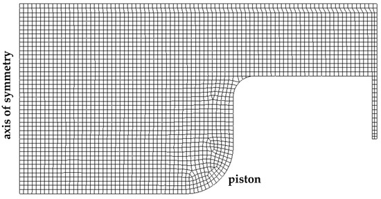
Figure 1.
Computational grid for the model validation at 30 CAD BTDC.
Based on the chamber’s geometry, the grid was fairly structured and uniform. Further, such a grid guaranteed acceptable values of y+ on the wall boundaries for the use of wall functions.
The grid employed between the head of the piston and the cylinder head was fully structured by using quadrilateral elements. The numerical domain, at the IVC, was composed of 16,346 numerical cells and 16,645 grid points and was generated by imposing an average cell size equal to 0.5 mm. The crevice, with a thickness of 0.6 mm, consisted of two rows of 0.3-mm numerical cells to guarantee a good accuracy. The grid motion was carried out by means of a layering technique.
The model was validated based on the experimental data available in [12] for the case without ozone and an intake mixture temperature of 473 K. A perfectly homogeneous mixture containing iso-octane and air was considered at the IVC, with a 10% mass fraction of CO2 and H2O, to take into account the residuals that remained trapped in the dead space between one work cycle and the next. The mass fractions of residuals were computed from both the equivalence ratio and the stoichiometry of a single global combustion reaction. Hence, the actual equivalence ratio based on the total mass at the IVC was slightly lower than the theoretical value of 0.3. The initial pressure and temperature of the gas mixture in the cylinder were selected based on the gas conditions in the intake duct and on the basis of a thermodynamic analysis of the total heat released. The wall temperature was assumed to be equal to 450 K and kept constant during the simulation. Such a value was chosen based on the temperature of the preheated gas mixture and by performing a parametric analysis in order to match the experimental pressure trace and heat release profile. The swirl ratio was set to 1 with a gas velocity linearly proportional to the distance from the cylinder axis (i.e., a rigid body profile). The initial values of the turbulent kinetic energy (k) and its dissipation rate (ϵ) could be determined by employing the following expressions [40]:
where and are constants equal to and , respectively; is the mean piston speed; is the angle, in radians, during which the intake valve remains open; and and are the piston area and the maximum open intake area, respectively.
The initial and boundary conditions are summarized in Table 2.
Table 2.
Initial and boundary conditions.
A time-dependence analysis was also carried out for the numerical time step and a value equal to 0.01 CAD was chosen to guarantee a good temporal accuracy. A spatial second-order upwind method for the convective terms and a centered second-order scheme for the diffusive terms were used, respectively. Chemistry was solved by directly integrating the system of ODEs [33].
3. Results and Discussion
3.1. Model Validation
The model can be validated by comparing the results in regards to in-cylinder pressure, heat release rate and cumulative heat release with the experimental measurements of [12], as shown in Figure 2 and Figure 3.
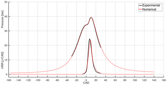
Figure 2.
Comparison between experimental and numerical results in terms of in-cylinder pressure and heat release rate (HRR).

Figure 3.
Comparison between experimental and numerical results in terms of cumulative heat release.
As shown in Figure 2, both the numerical pressure trace and the heat release profile followed the experimental data very closely. It is worth noting that the numerical profile of the heat release rate was computed by considering the enthalpy balance of each reaction of the kinetic reaction mechanism, whereas the experimental profile was obtained from the in-chamber pressure measurements by applying the first principle of thermodynamics. The computed in-cylinder pressure reproduced the measured pressure with great accuracy (i.e., a difference less than 1 bar for the entire range of the experimental data). The two-stage increase of pressure, which also occurred in the experimental case, was due to the fact that combustion occurred mainly after TDC. Up until TDC, the pressure mainly increased as a consequence of the piston’s motion. Combustion started at the beginning of the expansion stroke, with an increase of pressure caused by the heat released. The model was able to predict the mixture auto-ignition timing at about 9 CAD BTDC. The pressure peak was computed with excellent accuracy, both in terms of timing (10 CAD ATDC measured vs. 10.5 CAD ATDC computed) and value (39.3 bar measured vs. 39.38 bar computed). As regards the combustion process, the measured peak of heat release was and occurred around 7 CAD ATDC, whereas the computed peak occurred 1.2 CAD later with a heat release of . A further confirmation of the reliability of the model can be achieved by comparing the experimental and numerical cumulative heat release profiles, as shown in Figure 3. The total heat released at 30 CAD ATDC was 255 J from the measurements and 259 J from the simulation. This slight difference could have been related to the available experimental data up to 30 CAD ATDC. From the final slope of the experimental profile, it can be argued that the total heat released was somewhat larger. At EVO, the computed heat released was 264.5 J. The results show that the fuel burned almost completely; indeed only 4.76% of the initial iso-octane mass was present at EVO. The amount of unburned fuel was mainly located within the volume crevices, due to the low gas temperature in such volumes.
3.2. Influence of Piston Shape
3.2.1. Cup-in-Piston
The combustion process is highly dependent on the turbulent flow field in the engine chamber. The shape of the combustion chamber plays a fundamental role in driving the flow and enhancing turbulence in the chamber. As previously stated, combustion started at around 9 CAD BTDC, with the gas temperature in the piston cup fairly uniform and equal to about 1130 K. However, the influence of gas turbulence levels on the heat release, temperature and pressure were more clearly evident near TDC.
Figure 4 shows the gas temperature distribution at TDC. Fuel starts to burn in the middle of the combustion chamber, which is contrary to what one would expect from the uniform temperature distribution before auto-ignition. This is due to the interaction between chemistry and turbulence. The results show that even if the gas mixture temperature was high enough in the piston cup for the ignition to occur, combustion was relatively slow in regions with higher turbulence levels.
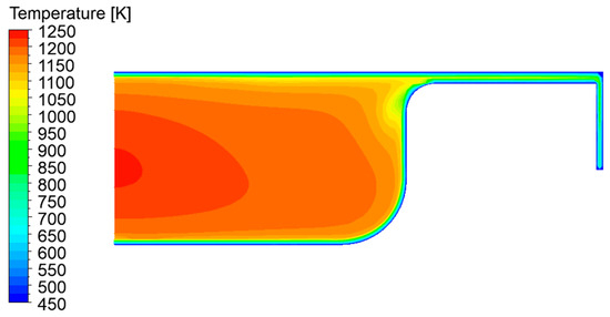
Figure 4.
Gas temperature distribution at TDC.
This is well explained in Figure 5, where the scatter plots of turbulent diffusivity as a function of temperature for each computational cell at several crank angles are shown.
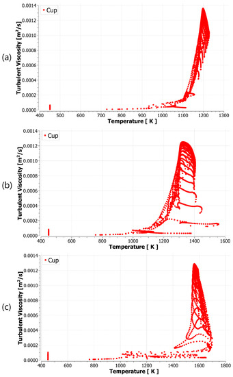
Figure 5.
Scatter plots of the turbulent diffusivity as a function of gas temperature at different crank angles: (a) TDC; (b) 5 CAD ATDC; (c) 10 CAD ATDC.
Figure 5a, which refers to TDC, shows that the regions in the piston cup where chemical reactions proceeded faster at the start of combustion were characterized by a turbulent diffusivity of about and a temperature of about 1225 K. The maximum value of turbulent diffusivity at TDC was , which corresponds to a temperature of about 1190 K. The influence of turbulence on the combustion process was even stronger when considering the situations at 5 and 10 CAD ATDC in Figure 5b,c, respectively. The figure shows that the combustion process sped up when turbulent diffusivity was low. For instance, at 5 CAD ATDC, chemical reactions were promoted by values of turbulent diffusivity of about .
Figure 6 shows the contour plots of gas mixture turbulent diffusivity and temperature at 10 CAD ATDC. It can be observed that the regions characterized by a compromise between turbulence and temperature for a fast combustion were those nearest to the piston wall. The peak of the heat release rate occurred at this crank angle. On the other hand, in the middle of the chamber, the chemical reactions resulted in a lower heat release rate.
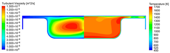
Figure 6.
Turbulent gas diffusivity (left) and temperature (right) contour plots at 10 CAD ATDC.
3.2.2. Flat Piston
The engine used in [12] was a diesel engine with a cup-in-piston geometry used to increase turbulence and enhance combustion. Specifically, the cup in the piston causes a squish during compression (especially near TDC) and a bulk flow recirculation in the cup. In order to understand the impact of such a flow structure on HCCI combustion, a simulation was carried out by using a flat piston, whose computational grid is shown in Figure 7. The grid resolution is the same as that of the previous engine. Initial and boundary conditions are the same as in the previous case.
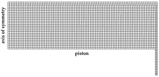
Figure 7.
Computational grid for the engine with a flat piston at 30 CAD BTDC.
The results show that for this case a faster combustion occurred. Indeed, Figure 8 shows a similarity between the case with the cup-in-piston and the case with the flat piston in terms of heat release rates and pressure profiles. Although the ignition timing is roughly comparable for both cases, combustion proceeded much faster for the flat-piston case. HRR reached a peak value of at 1.64 CAD ATDC, which is 6.76 CAD more advanced and increased compared to the cup-in-piston case. As a consequence, the pressure peak was 4.57 CAD more advanced, with an increase of 10.46 bar. This result is in agreement with the numerical findings of [41], where the combustion process of an HCCI engine was analyzed using different values of the initial turbulent diffusivity.
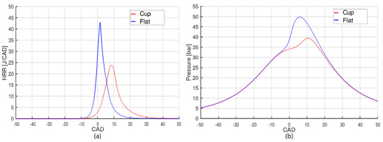
Figure 8.
Results obtained for the two piston shapes: (a) heat release rate; (b) in-cylinder pressure.
As regards the total heat released, for the flat-piston case, the energy released from combustion was 278 J, which was 5% higher than the cup-in-piston case. This increase was due to both a higher amount of burned fuel and a more complete combustion. Only 2.54% of the initial mass of iso-octane was left at EVO, which was about half of the amount of unburned fuel mass in the cup-in-piston case. Moreover, a larger amount of carbon dioxide and water were found within the exhaust gas in the flat-piston case, with a mass of carbon monoxide five times lower than that of the cup-in-piston case.
In order to assess the turbulence–chemistry interaction, Figure 9 shows the scatter plots of turbulent diffusivity versus temperature for the two engines at three different crank angles (i.e., 10, 5 and 3 CAD BTDC).
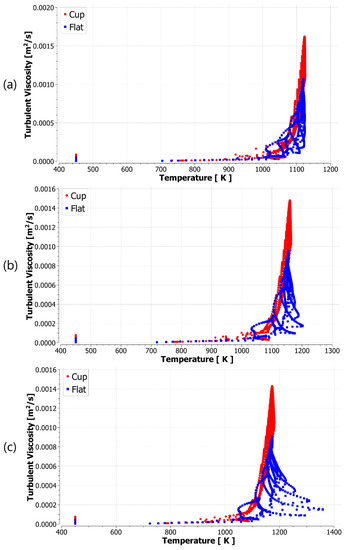
Figure 9.
Comparison between the scatter plots of the turbulent diffusivity as a function of gas temperature for the two piston shapes at different crank angles: (a) 10 CAD BTDC; (b) 5 CAD BTDC; (c) 3 CAD BTDC.
The results show that the maximum turbulent diffusivity at 10 CAD BTDC was 37.5% lower in the flat-piston case than in the cup-in-piston case, while the gas temperature was approximately the same. As with the cup-in-piston case, the combustion started in the middle of the combustion chamber, but it proceeded faster than that of the cup-in-piston case since the turbulence intensity was lower. Indeed, Figure 9a shows that the numerical cells with a higher temperature (T > 1100 K) were characterized by a turbulent diffusivity ranging from to for the cup-in-piston case, and from to for the flat-piston case. As shown in Figure 9b,c, this favorable compromise between turbulence and temperature accelerated the combustion process more rapidly in the flat-piston case. Figure 9c indicates that a turbulent diffusivity of about is the optimal condition for combustion, which is the same optimal condition promoting combustion in the original engine geometry.
In order to discover the region of the chamber in which the combustion initially takes place, Figure 10 shows the gas turbulent diffusivity and temperature contour plots at 9 and 3 CAD BTDC, respectively. The distribution of turbulent diffusivity was not perfectly symmetrical with respect to the middle plane between the piston and the head. Specifically, in the region where gas temperature increased, the turbulent intensity assumed the optimal value . Therefore, combustion started almost uniformly in the combustion chamber at about 9 CAD BTDC, as shown in Figure 10a, then proceeded with greater speed in the region with lower turbulence intensity and moved towards the piston and engine axis, as shown in Figure 10b.
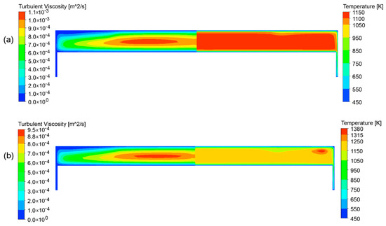
Figure 10.
Turbulent diffusivity (left) and temperature (right) distributions at different crank angles for the flat-piston case. (a) 9 CAD BTDC; (b) 3 CAD BTDC.
3.3. Influence of Swirl Motion
It is well known that a swirl motion in an engine affects the turbulence level distribution in the combustion chamber. In order to investigate the role of the swirl on combustion, simulations were carried out without swirl by employing the flat-piston engine with the same initial and boundary conditions. Specifically, the values of k and ε at IVC were kept the same as in the simulations with swirl. Therefore, the no-swirl simulations were aimed to understand how the absence/presence of a swirl motion influences turbulence distribution, then combustion, in the engine chamber.
Figure 11 shows the heat release and in-cylinder pressure profiles with and without swirl. The absence of swirl led to a slower combustion. Indeed, the maximum value of heat release rate decreased by 11.7 J/CAD and occurred 4.16 CAD later than the swirl case, leading to a 5 bar reduction and a 3.07 CAD delay of the pressure peak. The total heat released was the same for both cases with and without swirl, as was the amount of unburned fuel at EVO.
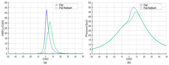
Figure 11.
Results obtained for the two flat cases: (a) heat release rate; (b) in-cylinder pressure.
The different profiles of Figure 11 are related to different turbulent diffusivities during the combustion process. Figure 12 shows a comparison between the two cases (i.e., with and without swirl) in terms of turbulent diffusivity distribution at 15 CAD BTDC. The maximum value of turbulent diffusivity was equal to for the case without swirl and for the case with swirl. Indeed, the swirl motion dissipated the initial turbulent kinetic energy more rapidly during the compression stroke. Since the turbulent diffusivity was higher without swirl motion, and considering the results of the previous sections, it can be concluded that combustion proceeds slower without swirl.
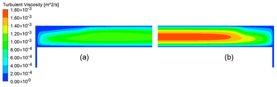
Figure 12.
Turbulent diffusivity distribution at 15 CAD BTDC in the case with a flat piston: (a) with swirl; (b) without swirl.
The lower combustion rate for the case without swirl resulted in a lower temperature rise. Figure 13 shows the scatter plots of the turbulent diffusivity versus temperature at 5 CAD BTDC and 5 CAD ATDC for the two cases. At 5 CAD BTDC, the maximum temperatures in the chamber were 1202 K and 1148 K for the cases with and without swirl, respectively. At this crank angle, the optimal value of turbulent diffusivity that promoted a faster combustion for the case without swirl was closer to the walls. Since the influence of the low temperature near the walls was still predominant compared to the low turbulence levels, combustion started in the middle of the chamber, as shown in Figure 14. The figure shows the gas temperature distribution at 7 CAD BTDC.
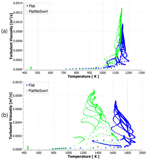
Figure 13.
Comparison between the scatter plots of the turbulent diffusivity as a function of gas temperature for the cases with and without swirl: (a) 5 CAD BTDC; (b) 5 CAD ATDC.
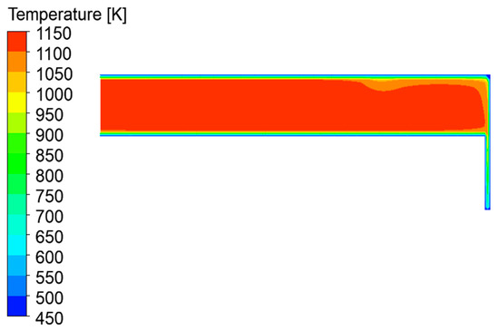
Figure 14.
Temperature distribution at 7 CAD BTDC without swirl.
The heat of combustion was mainly released in the center region of the cylinder, but at a low rate due to high turbulence levels, until the gas mixture temperature was sufficiently high in the low turbulence regions (i.e., regions closer to walls). Combustion then also proceeded in those regions, and the entire combustion chamber was involved in the process, except for the crevices. As in the previous cases, a sudden increase in the combustion rate occurred in the regions where the turbulent diffusivity was between 1 and , as shown in Figure 13b.
Figure 15 shows the gas temperature distribution in the engine chamber at 3 CAD BTDC. Two temperature regions are depicted where reactions occurred more rapidly. The first one, indicated with (I) in Figure 15, was located in the center of the combustion chamber; the second region, indicated with (II), was smaller and located closer to the liner. The latter was also visible in the flat-piston case with swirl (shown in Figure 10b) at higher gas temperatures, since the combustion evolved faster. Indeed, at 1 CAD BTDC, the temperature was still quite uniform, equal to about 1180 K in both high () and low turbulence () regions. Starting from TDC, combustion was favored within low turbulence regions. This is shown both in the scatter plot of Figure 13b at 5 CAD ATDC, and in Figure 16, where temperature distribution can be seen at 8 CAD ATDC.
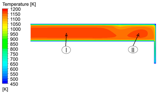
Figure 15.
Temperature distribution at 3 CAD BTDC for the flat-piston case without swirl.
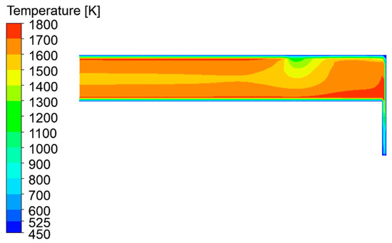
Figure 16.
Temperature distribution at 8 CAD ATDC without swirl.
3.4. Performance and Emissions
In this section, the three previous engine configurations (i.e., cup-in-piston with swirl, flat-piston with swirl and flat-piston without swirl) are compared in terms of engine performance and emissions. At first, heat release rate profiles are analyzed for the three cases, then the gross indicated work per cycle is computed and finally emissions are compared for the three configurations.
3.4.1. Heat Release Rate
Figure 17 shows the heat release rate profiles for the three configurations. The heat release of the flat-shaped piston geometry without swirl initially followed that of the case with the cup-in-piston. Indeed, the mixture temperature and turbulent diffusivity were very similar until auto-ignition. During the final part of the compression stroke, however, the cup-shaped piston geometry generated a squish and a bulk recirculation zone. Thus, the turbulent diffusivity did not dissipate as fast as for the case with the flat-piston engine geometry.
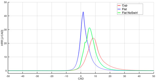
Figure 17.
Heat release rate for the three cases.
At 10 CAD BTDC, the maximum turbulent diffusivities were for the cup-in piston engine and for the flat-piston engine without swirl, whereas at TDC they decreased by 16% and 32%, respectively. This turbulence decrease involved the entire combustion chamber, and therefore several low turbulence regions where combustion accelerated were depicted for the flat-piston case with swirl, leading to a rise in HRR compared to the case with a cup.
For the flat-piston case without swirl, an HRR local maximum could be observed at 3 CAD ATDC, before starting to rise again shortly after. This trend may have been due to some low turbulence regions close to the walls, where combustion was initially favored, but the fuel/air mixture stopped burning due to relatively low temperatures in the surroundings. Indeed, for this case, as previously mentioned, the optimal levels of turbulent diffusivity for combustion were located closer to walls than for the case with swirl.
In addition to the HRR profiles, CA10, CA50 and CA90 (i.e., the crank angles when 10%, 50% and 90% of the total heat has been released, respectively) were computed. Table 3 summarizes the values for the three cases and the combustion duration, which was defined as the difference between CA90 and CA10.
Table 3.
CAx crank angles when x% of total heat has been released, and combustion duration for three cases analyzed.
From Table 3 and Figure 18, it can be seen that for the flat-piston engine with swirl, combustion proceeded faster with respect to the other two cases. Indeed, for this case, CA10 occurred before TDC, and the combustion duration was 9.59 CAD, which is 5.89 CAD and 1.41 CAD faster than the cup-in-piston and flat piston without swirl cases, respectively. Furthermore, it can be observed that the heat between CA50 and CA90 was released at about the same rate for the two flat-piston cases. On the other hand, for the cup-in-piston case, the entire process of combustion was slower and ended much later than for the flat-piston cases. These results are in agreement with other works available in the literature [21,22,23]. Specifically, reduction of the combustion duration for the case of a flat-piston engine has been determined both experimentally and numerically for this type of engines.
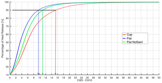
Figure 18.
Percentage of total heat release for the three cases. The value on the x-axis identified by the arrows represents the combustion duration.
Figure 18 shows the ratio between the cumulative heat release and the total heat release as a function of CAD, referring to CA10 for all cases. The combustion durations are also shown in the figure.
3.4.2. In-Cylinder Pressure Profiles and Gross Indicated Work
Figure 19 shows the in-cylinder pressure profiles for the three cases. For the flat-piston case with swirl, the pressure peak was equal to 49.85 bar and occurred at 6.03 CAD ATDC. This peak had an increase of 26.84% and an advance of 3.97 CAD with respect to the cup-in-piston with swirl case. This was due to both a shorter combustion duration and because a significant part of the heat was released before TDC. The pressure profile for the flat-piston geometry without swirl was in between the other two cases, with a pressure peak equal to 44.82 bar at 9.1 CAD ATDC.
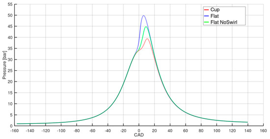
Figure 19.
Pressure profiles for the three cases.
The gross indicated work per cycle, , defined as the work delivered to the piston over the compression and expansion strokes, is computed as:
and given in Table 4.
Table 4.
Gross indicated work per cycle for the three cases.
The table shows that the flat-piston engines with and without swirl provided work increases of 9.64% and 8.59%, respectively, when compared to the cup-in-piston engine.
3.4.3. Emissions
Engine emissions were evaluated at 140 CAD ATDC, which corresponded to the exhaust valve opening. Measurements in terms of emissions of the main pollutants are not available, so a comparative analysis of the numerical results of the three cases is performed in this section, in order to give useful insights in terms of trends and to investigate the influence of combustion on emissions. Table 5 shows the amounts of the main pollutant species for the three cases, given in grams per kilogram of fuel.
Table 5.
Emissions at EVO .
Carbon oxides and UHCs depend on the completeness of the combustion process, and based on previous considerations a decrease in carbon monoxide and UHCs was expected for the flat-piston cases compared to the cup-in-piston case. Specifically, the amount of CO decreased by 86.79% and 80.65% for the flat piston with and without swirl cases, respectively.
The main chemical species of UHCs was unburnt iso-octane for all cases. A fuel fraction was trapped in the crevices, where temperature was relatively low. However, like the carbon monoxide, there were 56.05% and 55.21% less UHCs for the cup-in-piston case when compared to the flat-piston cases with and without swirl, respectively. A more complete combustion leads to an increase of CO2. For the three cases, the amount of carbon dioxide was comparable, with increases of 6.90% and 6.59% for the flat-piston cases with and without swirl, respectively, compared to the cup-in-piston case.
As regards nitrogen oxides, the most significant differences were in terms of nitrogen monoxide, with increases of 401% and 185% for the flat-piston cases with and without swirl, respectively, compared to the cup-in-piston case. Nitrogen oxides depend on the in-chamber temperature. Indeed, higher temperatures enhance the production of NO, whereas lower temperatures facilitate the complete oxidation of nitrogen to form NO2. The NO emissions, therefore, were related to the maximum temperature of 1778 K for the cup-in-piston case, whereas the in-chamber maximum temperatures were 1909 K and 1794 K for the flat-piston cases with and without swirl, respectively. Although the maximum temperature reached was comparable for both the cup-in-piston case and the flat-piston case without swirl, in the latter case a larger amount of fluid mass was involved at this high temperature. This difference in mass justified the increase of NO concentration for the flat-piston case without swirl.
4. Conclusions
In this work, the role of the turbulent flow structure in an HCCI engine has been analyzed in terms of engine performance and emissions by considering the influence of the geometry of the combustion chamber and of swirl motion. A reduced kinetic mechanism and EDC combustion model were used to perform this investigation. The model was able to accurately reproduce experimental data in terms of in-cylinder pressure and heat release profiles. In agreement with other works where different combustion models have been used, the increase of turbulence intensity in an HCCI engine led to a longer combustion duration. The final considerations are:
- combustion is favored in regions of the engine chamber characterized by temperatures of at least 1100 K and a turbulent diffusivity of about ;
- a swirl motion dissipates turbulence more rapidly during the compression stroke, thus favoring the occurrence of combustion;
- a flat-piston geometry provides a shorter combustion duration and an advance of the HRR peak timing with respect to cup-in-piston geometry. This is due to the decrease of turbulence intensity in the chamber, which leads to a faster combustion;
- the net gross work delivered to the piston over the compression and expansion strokes increases with a flat-piston geometry. Such an increase is larger for cases without swirl due to the increase of the in-cylinder pressure during the first part of the expansion stroke;
- UHCs and CO emissions decrease under flat-piston geometry due to a more complete combustion. The maximum reduction is in terms of carbon monoxide.
Based on such considerations, it can be concluded that, for the HCCI engine under examination, the flat-piston geometry provides better performance than the cup-in-piston geometry. Although the presence of a swirl motion reduces the combustion duration, a slight increase in the gross indicated work per cycle was observed. CO2, NO2 and UHCs emissions are only slightly influenced by the swirl, whereas CO decreases and NO increases. However, the flat-piston case without swirl should be preferred in order to limit the maximum value of the in-cylinder pressure.
Further investigations are needed to extend these analyses to HCCI engines operating under different equivalence ratios and compression ratios, among others. Such analyses would be useful to in order to verify if the thermofluid-dynamic conditions that have favored combustion in this work are still valid or they change as a function of other parameters. Furthermore, a validation of the numerical model in terms of emissions of the main pollutants would be useful to make the model a predictive tool to quantify the composition of exhaust gases.
Author Contributions
Conceptualization, A.V. and V.M.; Data curation, M.D.; Formal analysis, M.D.; Funding acquisition, V.M.; Investigation, M.D. and A.V.; Methodology, M.D.; Project administration, A.V. and V.M.; Resources, A.V. and V.M.; Software, M.D.; Supervision, A.V. and V.M.; Validation, M.D.; Visualization, M.D.; Writing–original draft, M.D.; Writing, review and editing, A.V. and V.M. All authors have read and agreed to the published version of the manuscript.
Funding
This research was funded by MIUR-“Ministero dell’Istruzione, dell’Università e della Ricerca” under project EXTREME-“Innovative technologies for EXTREMely Efficient spark ignited engines”, ARS01_00849.
Conflicts of Interest
The authors declare no conflict of interest.
References
- Heywood, J.B. Internal Combustion Engine Fundamentals; McGraw-Hill Inc.: New York, NY, USA, 1988. [Google Scholar]
- Bendu, H.; Murugan, S. Homogeneous Charge Compression Ignition (HCCI) Combustion: Mixture Preparation and Control Strategies in Diesel Engines. Renew. Sustain. Energy Rev. 2014, 38, 732–746. [Google Scholar] [CrossRef]
- Hasan, M.M.; Rahman, M.M. Homogeneous Charge Compression Ignition Combustion: Advantages over Compression Ignition Combustion, Challenges and Solutions. Renew. Sustain. Energy Rev. 2016, 57, 282–291. [Google Scholar] [CrossRef]
- Sharma, T.K.; Rao, G.A.P.; Murthy, K.M. Homogeneous Charge Compression Ignition (HCCI) Engines: A Review. Arch. Comput. Method. E 2016, 23, 623–657. [Google Scholar] [CrossRef]
- Dec, J.E.; Sjöberg, M. Isolating the Effects of Fuel Chemistry on Combustion Phasing in an HCCI Engine and the Potential of Fuel Stratification for Ignition Control. SAE Tech. Pap. 2004. [Google Scholar] [CrossRef]
- Yao, M.; Zheng, Z.; Liu, H. Progress and Recent Trends in Homogeneous Charge Compression Ignition (HCCI) Engines. Prog. Energy Combust. 2009, 35, 398–437. [Google Scholar] [CrossRef]
- Saxena, S.; Bedoya, I.D. Fundamental phenomena affecting low temperature combustion and HCCI engines, high load limits and strategies for extending these limits. Prog. Energy Combust. 2013, 39, 457–488. [Google Scholar] [CrossRef]
- Peng, Z.; Zao, H.; Ma, T.; Ladommatos, N. Characteristics of Homogeneous Charge Compression Ignition (HCCI) Combustion and Emissions of n-Heptane. Combust. Sci. Technol. 2005, 177, 2113–2150. [Google Scholar] [CrossRef]
- Gowthaman, S.; Sathiyagnanam, A.P. Analysis the Optimum Inlet air Temperature for Controlling Homogeneous Charge Compression Ignition (HCCI) Engine. Alex. Eng. J. 2018, 57, 2209–2214. [Google Scholar] [CrossRef]
- Tanaka, S.; Ayala, F.; Keck, J.C.; Heywood, J.B. Two-stage ignition in HCCI combustion and HCCI control by fuels and additives. Combust. Flame 2003, 132, 219–239. [Google Scholar] [CrossRef]
- Foucher, F.; Higelin, P.; Mounaїm-Rousselle, C.; Dagaut, P. Influence of ozone on the combustion of n-heptane in a HCCI engine. Proc. Combust. Inst. 2013, 34, 3005–3012. [Google Scholar] [CrossRef]
- Masurier, J.B.; Foucher, F.; Dayma, G.; Rousselle, C.; Dagaut, P. Application of an Ozone Generator to Control the Homogeneous Charge Compression Ignition Combustion Process. SAE Tech. Pap. 2015. [Google Scholar] [CrossRef]
- Masurier, J.B.; Foucher, F.; Dayma, G.; Dagaut, P. Homogeneous charge compression ignition combustion of primary reference fuels influenced by ozone addition. Energy Fuels 2013, 27, 5495–5505. [Google Scholar] [CrossRef]
- Masurier, J.B.; Foucher, F.; Dayma, G.; Dagaut, P. Investigation of iso-octane combustion in a homogeneous charge compression ignition engine seeded by ozone, nitric oxide and nitrogen dioxide. Proc. Combust. Inst. 2015, 35, 3125–3132. [Google Scholar] [CrossRef]
- Herold, R.; Krasselt, J.M.; Foster, D.E.; Ghandhi, J.B.; Reuss, D.L.; Najt, P.M. Investigations into the Effects of Thermal and Compositional Stratification on HCCI Combustion–Part II: Optical Engine Results. SAE Int. J. Engines 2009, 2, 1034–1053. [Google Scholar] [CrossRef]
- Viggiano, A.; Magi, V. An Investigation on the Performance of Partially Stratified Charge CI Ethanol Engines. SAE Tech. Pap. 2011. [Google Scholar] [CrossRef]
- Krasselt, J.M.; Foster, D.E.; Ghandhi, J.B.; Herold, R.; Reuss, D.L.; Najt, P.M. Investigations into the Effects of Thermal and Compositional Stratification on HCCI Combustion—Part I: Metal Engine Results. SAE Tech. Pap. 2009. [Google Scholar] [CrossRef]
- Yu, R.; Joelsson, T.; Bai, X.; Johansson, B. Effect of Temperature Stratification on the Auto-ignition of Lean Ethanol/Air Mixture in HCCI engine. SAE Tech. Pap. 2008. [Google Scholar] [CrossRef]
- Prasad, B.; Sharma, C.; Anand, T.; Ravikrishna, R. High Swirl-Inducing Piston Bowls in Small Diesel Engines for Emission Reduction. Appl. Energy 2011, 88, 2355–2367. [Google Scholar] [CrossRef]
- Abdul Gafoor, C.P.; Gupta, R. Numerical Investigation of Piston Bowl Geometry and Swirl Ratio on Emission From Diesel Engines. Energy Convers. Manag. 2015, 101, 541–551. [Google Scholar] [CrossRef]
- Kong, S.C.; Reitz, R.D.; Christensen, M.; Johansson, B. Modeling the Effects of Geometry Generated Turbulence on HCCI Engine Combustion. SAE Tech. Pap. 2003. [Google Scholar] [CrossRef]
- Christensen, M.; Johansson, B.; Hultqvist, A. The Effect of Combustion Chamber Geometry on HCCI Operation. SAE Tech. Pap. 2002. [Google Scholar] [CrossRef]
- Vressner, A.; Hultqvist, A.; Johansson, B. Study on Combustion Chamber Geometry Effects in an HCCI Engine Using High-Speed Cycle-Resolved Chemiluminescence Imaging. SAE Tech. Pap. 2007. [Google Scholar] [CrossRef]
- Magnussen, B.F. On the structure of turbulence and a generalized Eddy Dissipation Concept for chemical reaction in turbulent flow. In Proceedings of the 19th Aerospace Sciences Meeting, St. Louis, MO, USA, 12–15 January 1981. [Google Scholar] [CrossRef]
- Golovitchev, V.I.; Atarashiya, K.; Tanaka, K.; Yamada, S. Towards universal EDC-based combustion model for compression ignited engine simulations. SAE Tech. Pap. 2003. [Google Scholar] [CrossRef]
- Hong, S.; Assanis, D.; Wooldridge, M.S. Multi-Dimensional Modeling of NO and Soot Emissions with Detailed Chemistry and Mixing in a Direct Injection Natural Gas Engine. SAE Tech. Pap. 2002. [Google Scholar] [CrossRef]
- Sinha, A.; Sivaprakasam, M.; Ravikrishna, R.V. Spray Vortex Interactions in a Trapped Vortex Combustor. In Proceedings of the 22nd National Conference on IC Engines and Combustion NIT-Calicut, Kerala, India, 10–13 December 2011. [Google Scholar]
- Emami, S.; Jafari, H.; Mahmoudi, Y. Effects of Combustion Model and Chemical Kinetics in Numerical Modeling of Hydrogen-Fueled Dual-Stage HVOF System. J. Therm. Spray Tech. 2019, 28, 333–345. [Google Scholar] [CrossRef]
- Parente, A.; Malik, M.R.; Contino, F.; Cuoci, A.; Dally, B.B. Extension of the Eddy Dissipation Concept forturbulence/chemistry interactions to MILD combustion. Fuel 2016, 163, 98–111. [Google Scholar] [CrossRef]
- Bao, H. Development and Validation of a New Eddy Dissipation Concept (EDC) Model for MILD Combustion. Master’s Thesis, Delft University of Technology, Delft, The Netherlands, 2017. [Google Scholar]
- Grimsmo, B.; Magnussen, B.F. Numerical Calculation of Turbulent Flow and Combustion in an Otto Engine Using the Eddy Dissipation Concept. In Proceedings of the Comodia 90, Kyoto, Japan, 3–5 September 1990. [Google Scholar]
- Hong, S.; Wooldridge, M.S.; Im, H.G.; Assanis, D.N.; Kurtz, E. Modeling of Diesel Combustion, Soot and NO Emissions Based on a Modified Eddy Dissipation Concept. Combust. Sci. Technol. 2008, 180, 1421–1448. [Google Scholar] [CrossRef]
- Ansys® Academic Research CFD. Available online: http://www.ansys.com/academic (accessed on 11 October 2020).
- Bösenhofer, M.; Wartha, E.M.; Jordan, C.; Harasek, M. The Eddy Dissipation Concept—Analysis of Different Fine Structure Treatments for Classical Combustion. Energies 2018, 11, 1902. [Google Scholar] [CrossRef]
- Ertesvåg, I.S.; Magnussen, B.F. The Eddy Dissipation Turbulence Energy Cascade Model. Combust. Sci. Technol. 2007, 159, 213–235. [Google Scholar] [CrossRef]
- Magnussen, B.F. The Eddy Dissipation Concept—A Bridge between Science and Technology. In Proceedings of the ECCOMAS Thematic Conference on Computational Combustion, Lisbon, Portugal, 21–24 June 2005. [Google Scholar]
- Gran, I.R.; Magnussen, B.F. A Numerical Study of a Bluff-Body Stabilized Diffusion Flame. Part 2. Influence of Combustion Modeling and Finite-Rate Chemistry. Combust. Sci. Technol. 1996, 119, 191–217. [Google Scholar] [CrossRef]
- Luong, M.B.; Luo, Z.; Lu, T.F.; Chung, S.H.; Yoo, C.S. Direct numerical simulations of the ignition of lean primary reference fuel/air mixtures under HCCI condition. Combust. Flame 2013, 160, 2038–2047. [Google Scholar] [CrossRef]
- Saxena, P.; Williams, F.A. Numerical and Experimental Studies of Ethanol Flames. Proc. Combust. Inst. 2007, 31, 1149–1156. [Google Scholar] [CrossRef]
- Viggiano, A.; Magi, V. A comprehensive investigation on the emissions of ethanol HCCI engines. Appl. Energy 2012, 93, 277–287. [Google Scholar] [CrossRef]
- Viggiano, A.; Magi, V. Multidimensional Simulation of Ethanol HCCI Engines. SAE Tech. Pap. 2009. [Google Scholar] [CrossRef]


Publisher’s Note: MDPI stays neutral with regard to jurisdictional claims in published maps and institutional affiliations. |
© 2020 by the authors. Licensee MDPI, Basel, Switzerland. This article is an open access article distributed under the terms and conditions of the Creative Commons Attribution (CC BY) license (http://creativecommons.org/licenses/by/4.0/).