Abstract
The LLC resonant converter has been widely used in direct current (DC) power supply applications. However, fundamental harmonic approximation or other simplified analyses will introduce inevitable deviations. Therefore, the differential equation model with numerical solution of the LLC converter is proposed in this paper based on the operational principle of the ideal case. In order to solve the differential equation, initial values need to be substituted. The accurate LLC model based on time interval analysis is very complicated and cannot be used. In this paper, solution methods of the initial values corresponding to different switching frequencies are proposed. The initial values can be solved conveniently. Furthermore, the voltage gain curve is modified by the idealized analysis. Lastly, all the above research is verified by PSIM simulation. The work is helpful to understand the operational principle of the LLC resonant converter.
1. Introduction
The LLC resonant converter has many advantages such as isolation, adjustable voltage, and soft-switching characteristics [1,2]. Usually, it operates under the frequency modulation control strategy with half duty cycle. There are many analysis methods for the LLC resonant converter. The frequency-domain method is known as the fundamental harmonic approximation (FHA), which is the conventional analysis method of LLC [3,4]. But this method only analyzes the fundamental component and will introduce inevitable significant errors.
The state-plane method with state-trajectory is clear and useful to analyze the resonant converter. In [5], the 3D state-space trajectory of the LLC converter is simplified to a 2D state-plane trajectory by projection. Based on this work, the analysis and control methods of load transient, soft-start, and over-load protection are proposed [6,7]. The initial values of voltages and currents need to be acquired in the methods. However, there is no discussion on the solution of the initial values.
The time-domain method can be used to analyze the waveforms of periodic resonant current and voltage. The root-mean-square (RMS) value of the primary-side current can be calculated [8]. Due to the high circuit order of LLC, it is difficult to get the time domain solution. Therefore, simplified analysis has often been used in previous studies. In the simplified analysis, the value of the magnetizing inductance is assumed to be large and the magnetizing current remains unchanged in the freewheeling stage [9]. Another simplified method assumes the resonant capacitor is large enough so that its voltage remains unchanged in the freewheeling stage [10]. Calculated results with the above two simplified methods can not reflect the actual operating conditions of the LLC converter.
Numerical solution is another time-domain analysis method for the high order circuits. The differential equation model of the LLC resonant converter with parasitic components is solved in [11]. However, there is also a lack of analysis and calculation of the initial values. It is necessary to analyze the operating principle of the LLC converter correctly.
The accurate LLC model is proposed based on the generalized analysis of the operation modes. The model equations are derived from the current and voltage boundary conditions between stages to describe the circuit behavior [12,13]. The time interval analysis of the LLC converter is proposed in [14], and the equation system contains a certain number of trigonometric functions. Although they are both analyzed in the ideal case, the calculations are very complicated and difficult to be applied. The defined variables are different to each other. It is hard to transform the equation systems into other forms accurately.
In [10], the modified gain model and the corresponding design method are also proposed. The comparison results are based on the FHA method, which is just an approximation. The experimental verification is only conducted under different loads. More work on other operational conditions needs to be researched.
This paper presents a differential equation model of the LLC resonant converter in the ideal case. Section 2 establishes the model at the resonant frequency. Section 3 and Section 4 establish the model above and below the resonant frequency, respectively. The solution methods of initial values under different switching frequencies are described. The numerical solution is calculated through the MATLAB software. The simulation results by PSIM software are given for verification. The modification of the voltage gain curve is shown in Section 5. Lastly, conclusions are given in Section 6.
2. LLC Converter Model at Resonant Frequency
In the ideal case, the circuit diagram of the full-bridge LLC resonant converter is shown in Figure 1. The resonant network consists of the resonant inductance Lr, the resonant capacitance Cr, and the magnetizing inductance Lm of the transformer. The turns ratio of the transformer is N. Ideally, parasitic parameters in the converter devices and the influences of the dead time of switches are ignored.
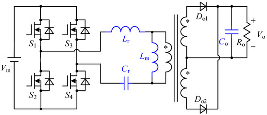
Figure 1.
The circuit of LLC resonant converter in the ideal case.
The resonant inductance and capacitance oscillate to transfer energy with unity voltage gain when the LLC resonant converter operates at the resonant frequency. In previous relevant references, it is usually assumed that the output capacitance is large enough, and the output voltage remains constant. In this paper, the output capacitance Co is considered to acquire a more accurate model. Therefore, the fourth-order differential equation model needs to be established. Since the duty cycle of LLC is fixed to 50%, the resonant tank waveforms in one half switching cycle are symmetrical in the reverse direction to the other half. Only the positive half cycle is discussed in this paper to simplify the analysis.
2.1. Differential Equation Model
When the LLC converter operates at the resonant frequency, the switching frequency fs is equal to resonant frequency fr, and the switching period is Tr. The waveforms of the converter are shown in Figure 2. vAB represents the voltage between the midpoints in the primary-side H-bridge.
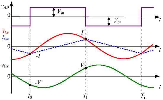
Figure 2.
Waveforms of LLC resonant converter at resonant frequency in the ideal case.
In the stage of (t0, t1), the equivalent circuit of LLC is shown in Figure 3. The energy is transferred directly from the primary-side to the secondary-side in this stage.

Figure 3.
Equivalent circuit of LLC resonant converter in the positive half cycle.
The expressions of inductance currents and capacitance voltages are listed as follows:
2.2. Solution of Initial Value
In order to calculate the numerical solution of the differential equations, it is necessary to solve the initial value of the switching cycle first. Assuming Zr1 is the characteristic impedance, and ωr1 is the resonant angular frequency:
At t1, it is assumed that the current iLr(t) is I, and vCr(t) is V. There is no current flowing through the secondary-side of transformer. The magnetizing current is exactly equal to the resonant current. By the symmetry principle, the current iLr(t) is −I, and the voltage vCr(t) is −V at t0.
The expressions of the resonant variables are given by:
The state-trajectory of iLr(t) and vCr(t) is drawn in the two-dimensional coordinate system as shown in Figure 4.

Figure 4.
The state-trajectory of LLC resonant converter at resonant frequency in the ideal case.
In the positive half switching cycle, iLm(t) changes from −I to I, thus:
Assuming the radius of the state-trajectory in Figure 4 is R, the resonant variables can be written as:
The current difference between the resonant current and the magnetizing current is transmitted to the secondary-side to supply the load, and it satisfies:
Replacing iLr(t) and iLm(t) gives:
That is:
Gathering the equation for I from (5) and V from (9) results in a system of equations, which is presented as:
If the input and output conditions are known, I and V can be calculated from the equations above. The expressions of iLr(t) and vCr(t) can be solved. It is also possible to get the RMS value of the resonant inductance current as:
2.3. Numerical Solution and Simulation Results
In this paper, a fourth-order differential equation model of the LLC converter is extracted. When the circuit order is higher than two, it is hard to solve the time-domain solution or the sign solution through inverse Laplace transformation. To obtain a more accurate LLC resonant converter model, a simple mathematical iterative method to calculate the numerical solution of the differential equations is applied in this paper. First, the voltage and current equation is transferred into the form as:
In which X is the variable matrix, X = (iLr vCr iLm vo)T, A and B are the coefficient matrices. The solution is iterated according to the simplest iterative equation with fixed step length as:
where δ represents the iteration step length, and n represents the number of iterations.
The expression of the positive half period is rewritten into the matrix form of the differential equation as below:
Table 1 shows the parameters of LLC converter used in this paper. At resonant frequency, the input voltage Vin is NVo = 864 V. First, the circuit parameters are set in the MATLAB software. Then, the initial values are solved. The matrix form of the differential equation is imported, and the iterative values are calculated. Lastly, the time-domain waveforms and the state-trajectories of the voltage and current are drawn. The correctness of the model and calculation is verified with two different values of the quality factor Q, which is expressed as:

Table 1.
The parameters of LLC converter.
The time-domain waveforms and the state-trajectories at the resonant frequency with Q1 = 0.1831 and Q2 = 0.3662 are shown in Figure 5. The numerical solution of one and a half cycles is calculated by MATLAB. The waveforms of the second half cycle are mainly the same as that of the first half cycle. It indicates that the calculation results of the differential equation model and the initial values are both correct.
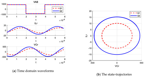
Figure 5.
MATLAB calculation results at resonant frequency.
Furthermore, PSIM simulation is used to verify the model and the numerical solution. Under the same circuit conditions, the waveforms are simulated, and the state-trajectories are drawn as Figure 6. It should be noted that the state-trajectories are nearly circular since the scales of the horizontal and vertical axes are different.

Figure 6.
PSIM simulation results of the state-trajectories at resonant frequency.
Comparing the MATLAB calculation results with the PSIM simulation results, the voltage and current changes in the LLC converter are mainly the same, and the state-trajectories are almost the same too. The differential equation model and the numerical solution is correct.
3. LLC Converter Model above the Resonant Frequency
3.1. Differential Equation Model
Ideally, when the voltage gain is less than the unity-gain, the switching frequency fs of the LLC resonant converter is above the resonant frequency fr. Assuming the switching period is Ts. There are two stages in half cycle at this condition, as shown in Figure 7, and they are named as positive resonant stage and negative resonant stage. The two stages both transmit energy from the input port to the load port. The equivalent circuit of positive resonant stage (t0, t1) is the same as Figure 3. The equivalent circuit of negative resonant stage (t1, t2) is shown in Figure 8.

Figure 7.
Waveforms of LLC resonant converter above resonant frequency in the ideal case.

Figure 8.
Equivalent circuit of the negative resonant stage of LLC resonant converter.
In the negative resonant stage, only the input voltage changes from Vin to −Vin, and the expression of voltage and current are as follows:
Then the expression is rewritten into the matrix form of the differential equation, as shown below:
The differential equations for the other half cycle can be listed similarly, which are not represented here.
3.2. Solution of Initial Value
Although there are two resonant stages in half cycle, the resonant devices are same, and the characteristic impedance and the resonant frequency are same. The analysis is relatively simple. It is assumed that the current iLr(t) is I1 and the voltage vCr(t) is V1 at time t2, and the current iLr(t) is I2 and the voltage vCr(t) is V2 at time t1. The length of time interval [t0, t1] is ∆t1, and the length of time interval (t1, t2) is ∆t2, as shown in Figure 7.
The state-trajectories of iLr(t) and vCr(t) are drawn in the two-dimensional coordinate system, as shown in Figure 9. To solve the values of these six variables, six equations are needed.

Figure 9.
The state-trajectory of LLC resonant converter above resonant frequency in the ideal case.
The magnetizing current increases linearly under the primary-side voltage of the transformer in the half cycle.
In the positive resonant stage, the state-trajectory can be written as:
The two instants t0 and t1 both satisfy the state-trajectory, and Equation (20) becomes:
From the state-trajectory, the time interval ∆t1 can be written as:
In the negative resonant stage, the state-trajectory can be written as:
The two instants t1 and t2 both satisfy the state-trajectory, and Equation (23) becomes:
From the state-trajectory, the time interval ∆t2 can be written as:
In the half cycle, the current difference between the resonant current and the magnetizing current transmits to the secondary-side to supply the load, and it satisfies:
Replace the variables and it becomes:
Gathering the equations above results in a system of equations that define these six unknown variables for the LLC converter above resonant frequency.
If the operational conditions with the input and output currents and voltages are known, V1, I1, V2, I2, ∆t1 and ∆t2 can be calculated using the MATLAB software. As there are inverse trigonometric functions in the equation, only the numerical solution can be solved instead of the sign solution.
3.3. Numerical Solution and Simulation Results
Using the same method in Section 2.3, the differential equation is imported into MATLAB, and the iterative values are calculated. The circuit parameters are the same as Table 1. The input voltage is set as 950 V, which is higher than NVo. The calculation results of one and a half cycles under two load conditions are shown in Figure 10.

Figure 10.
MATLAB calculation results above resonant frequency.
PSIM simulation is also used to verify the model and the numerical solution of the LLC converter above resonant frequency. Under the same load conditions, the state-trajectories are simulated as shown in Figure 11.
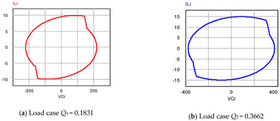
Figure 11.
PSIM simulation results of the state-trajectories above resonant frequency.
From the calculation results of MATLAB, the state-trajectories of the first cycle and the second half cycle basically coincide with each other. It shows that the calculation results are correct. The calculation method of initial values above resonant frequency presented in this paper is simple to use. Comparing the MATLAB calculation results with the PSIM simulation results, the voltage and current changes in the LLC converter are mainly the same, which verifies the correctness of the differential equation model.
4. LLC Converter Model below the Resonant Frequency
4.1. Differential Equation Model
The switching frequency fs of the LLC resonant converter is lower than the resonant frequency fr when the input voltage is lower than the transformed output voltage. There are two stages in the half cycle, named as the positive resonant stage and freewheeling stage. Only during the positive resonant stage, energy is transmitted from the input port to the load port. After the resonant inductance current is equal to the magnetizing inductance current, the rectifier diodes are reverse blocked. The waveforms are shown in Figure 12.

Figure 12.
Waveforms of LLC resonant converter below resonant frequency in the ideal case.
(t0, t1) is the positive resonant stage. The operational principle is same with the positive resonant stage shown in Section 3.1, and not listed anymore. (t1, t2) is the freewheeling stage. The equivalent circuit of the freewheeling stage is shown in Figure 13. Since the primary-side switches S1 and S4 are still ON, the input voltage of the resonant network is still Vin. The rectifier diode currents are zero, and the load is supplied by the output capacitance alone.

Figure 13.
Equivalent circuit of the freewheeling stage of LLC resonant converter.
In the freewheeling stage, the expressions of voltage and current are written as follows:
Then the above expressions are transformed into the matrix form of the differential equation, as shown below:
The differential equations for the negative half cycle can be listed similarly, which will not be repeated here.
4.2. Solution of Initial Value
When the switching frequency of the LLC resonant converter is lower than the resonant frequency, it is in the boost mode, and Vin < NVo. There are two stages in the half period. However, comparing with the mode above the resonant frequency, the operational principle is more complicated. This is because during the freewheeling stage, the rectifier diodes are OFF, and Lm is resonating with Lr and Cr. The new characteristic impedance Zr2 and the resonant angular frequency ωr2 are:
Similarly, the current iLr(t) is assumed to be I1, the voltage vCr(t) is V1 at time t2, the current iLr(t) is I2, the voltage vCr(t) is V2 at time t1, the length of time interval (t0, t1) is ∆t1. The length of time interval (t1, t2) is ∆t2. To represent the trajectories on the same state-plane, the trajectory of free-wheeling stage is compressed as an ellipse, as shown in Figure 14.

Figure 14.
The state-trajectory of LLC resonant converter below resonant frequency in the ideal case.
In the positive resonant stage below resonant frequency, the operational principle is same as the stage above resonant frequency. The state-trajectory is the same as Equations (20)–(22). As the free-wheeling stage is different from the other two stages, the other equations need to be listed differently.
During (t0, t1), the magnetizing current increases linearly under the voltage of the primary-side of the transformer that is equal to NVo.
In the free-wheeling stage, the state-trajectory can be written as
The two instants t1 and t2 both satisfy the state-trajectory, and Equation (33) becomes:
The time interval ∆t2 can be written as:
There is no current flowing through the rectifier diodes during [t1, t2]. Only the current difference between iLr and iLm in the time interval (t0, t1) is calculated when solving the output current.
Replace the variables and Equation (36) becomes:
Gathering the equations above results in a system of equations of LLC converter below resonant frequency. The numerical solution of V1, I1, V2, I2, ∆t1 and ∆t2 can be calculated by the MATLAB software with the operational conditions.
4.3. Numerical Solution and Simulation Results
The input voltage is set as 800 V, which is lower than the value of NVo. The differential equation with the circuit parameters of two different load conditions are imported into MATLAB. After calculating the initial values and the iterative values, the results of one and a half cycles below resonant frequency are shown in the paper as Figure 15.
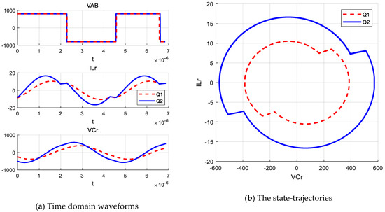
Figure 15.
MATLAB calculation results below resonant frequency.
Under the same load conditions, the LLC state-trajectories by PSIM simulation are shown as Figure 16. From the calculation results of MATLAB, the state-trajectories of the first cycle and the second half cycle of LLC below resonant frequency coincide with each other. Comparing the MATLAB calculation results with the PSIM simulation results, the initial values of voltage and current under different load conditions are basically the same, which verifies the correctness of the solution method of initial value. The PSIM simulation results show that the calculation results of the differential equation model are correct.

Figure 16.
PSIM simulation results of the state-trajectories below resonant frequency.
5. Modification of Voltage Gain Curve of LLC Converter
The initial values, which contain six parameters of the LLC resonant converter under different switching frequencies, are calculated easily in this paper. The calculated results can be used to modify the voltage gain curves of the LLC resonant converter theoretically. Three different load conditions are selected to calculate the voltage gains, which are Q1 = 0.1831, Q2 = 0.2441 and Q3 = 0.3662, respectively. The differential equation model with the initial value is used to solve the corresponding switching frequency by MATLAB. Comparisons between the results of the FHA method, MATLAB calculation, and the PSIM closed-loop simulation are listed in Figure 17. The limits of the gain curves are the maximum gain points of different load conditions, to make sure that the LLC converter is operating in the zero voltage switching (ZVS) zone. In addition, Table 2 shows the comparisons of switching frequencies of LLC converter at Q2 = 0.2441.

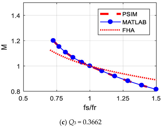
Figure 17.
The voltage gains curves of LLC converter with different Q values.
Table 2.
Comparisons of switching frequencies of LLC converter at Q2 = 0.2441.
The gain curves solved by MATLAB software using the differential equation model are almost the same as the PSIM simulation results. However, there are deviations between FHA and PSIM or MATLAB results. Below the resonant frequency, the voltage gains from FHA are lower than that of PSIM and MATLAB. In other words, the switching frequencies of FHA are lower than that of PSIM and MALTAB under the same voltage gains, as shown in Table 2. However, above resonant frequency, the voltage gains from FHA is higher than the other two curves in Figure 17. As only the fundamental component is considered, the switching frequency of FHA is far from the resonant frequency when Vin is far from NVo, and the deviation is large. With the differential equation model, the theoretical error of the FHA method is shown clearly in this paper.
It should be noticed that the PSIM and MATLAB results are both in the ideal case. The differences in voltage gain curves under different load conditions are not obvious. If considering the parasitic parameters, such as the ON resistors of the primary-side switches, the voltage gain curves in Figure 17 will be lower than that and the load should not be too light. If the load is too tight, the influence of parasitic parameters cannot be ignored anymore. The equivalent circuit will change greatly, and more work needs to be conducted.
6. Conclusions
The LLC resonant converter is analyzed using the numerical solution of the differential equation model. The main work is as follows:
- The differential equation models at, above and below the resonant frequency are built, respectively. The correctness of the differential equation model in the ideal case is verified by PSIM simulation.
- A novel numerical solution methods of the initial value with different switching frequencies are proposed, which can be calculated by MATLAB software easily. They can be used as a research foundation for other applications.
- The voltage gain curve is modified by the differential equation model, and it is almost the same as the PSIM simulation result in the ideal case. It can be used as the reference gain curve as a replacement of the curve acquired by the traditional FHA method.
However, all the pieces of research above are under the ideal condition. The complex operational principle of the LLC resonant converter with parasitic parameters in practical applications should be further studied.
Author Contributions
Conceptualization, F.L.; formal analysis, F.L. and H.L.; Funding acquisition, J.G.; investigation, H.L.; methodology, F.L.; resources, X.Y. and J.G.; software, S.L.; supervision, R.H. and X.Y.; validation, H.L. and S.L.; writing—original draft, S.L.; writing—review and editing, F.L. and R.H. All authors have read and agreed to the published version of the manuscript.
Funding
This research was funded by China Postdoctoral Science Foundation (grant no. 2019M650466), and Fundamental Research Funds for Beijing Technological Innovation and Service Capabilities (grant no. 77F1910913).
Conflicts of Interest
The authors declare no conflict of interest.
References
- Bhuvaneswari, C.; Babu, R.S.R. A review on LLC Resonant Converter. In Proceedings of the International Conference on Computation of Power, Energy Information and Communication (ICCPEIC), Chennai, India, 20–21 April 2016; pp. 620–623. [Google Scholar]
- Yang, B.; Lee, F.C.; Zhang, A.J.; Huang, G. Resonant converter for front end DC/DC conversion. In Proceedings of the APEC. Seventeenth Annual IEEE Applied Power Electronics Conference and Exposition (Cat. No.02CH37335), Dallas, TX, USA, 10–14 March 2002; Volume 2, pp. 1108–1112. [Google Scholar]
- Simone, S.D.; Adragna, C.; Spini, C.; Gattavari, G. Design-oriented steady-state analysis of LLC resonant converters based on FHA. In Proceedings of the International Symposium on Power Electronics, Electrical Drives, Automation and Motion (SPEEDAM), Taormina, Italy, 23–26 May 2006; pp. 200–207. [Google Scholar]
- Gu, Y.; Lu, Z.Y.; Hang, L.J.; Qian, Z.M.; Huang, G.S. Three-level LLC series resonant DC/DC converter. IEEE Trans. Power Electron. 2005, 20, 781–789. [Google Scholar] [CrossRef]
- Feng, W. State-Trajectory Analysis and Control of LLC Resonant Converters. Ph.D. Dissertation, Virginia Polytechnic Institute and State University, Blacksburg, VA, USA, 29 March 2013. [Google Scholar]
- Feng, W.; Lee, F.C.; Mattavelli, P. Simplified Optimal Trajectory Control (SOTC) for LLC Resonant Converters. IEEE Trans. Power Electron. 2013, 28, 2415–2426. [Google Scholar] [CrossRef]
- Feng, W.; Lee, F.C. Optimal Trajectory Control of LLC Resonant Converters for Soft Start-Up. IEEE Trans. Power Electron. 2014, 29, 1461–1468. [Google Scholar] [CrossRef]
- Lu, B.; Liu, W.; Liang, Y.; Lee, F.C.; Wyk, J.D. Optimal Design Methodology for LLC Resonant Converter. In Proceedings of the Twenty-First Annual IEEE Applied Power Electronics Conference and Exposition. APEC’06, Dallas, TX, USA, 3 March 2006; pp. 533–538. [Google Scholar]
- Ivensky, G.; Bronshtein, S.; Abramovitz, A. Approximate Analysis of Resonant LLC DC-DC Converter. IEEE Trans. Power Electron. 2011, 26, 3274–3284. [Google Scholar] [CrossRef]
- Liu, J.; Zhang, J.; Zheng, T.Q.; Yang, J. A Modified Gain Model and the Corresponding Design Method for an LLC Resonant Converter. IEEE Trans. Power Electron. 2017, 32, 6716–6727. [Google Scholar] [CrossRef]
- Li, F.; Hao, R.; Lei, H.; Zhang, X.; You, X. The influence of parasitic components on LLC resonant converter. Energies 2019, 12, 4305. [Google Scholar] [CrossRef]
- Fang, X.; Hu, H.; Shen, Z.J.; Batarseh, I. Operation Mode Analysis and Peak Gain Approximation of the LLC Resonant Converter. IEEE Trans. Power Electron. 2012, 27, 1985–1995. [Google Scholar] [CrossRef]
- Fang, X.; Hu, H.B.; Chen, F.; Somani, U.; Emil, A.; Shen, J.; Batarseh, I. Efficiency-Oriented Optimal Design of the LLC Resonant Converter Based on Peak Gain Placement. IEEE Trans. Power Electron. 2013, 28, 2285–2296. [Google Scholar] [CrossRef]
- Ettore, S.G.; Martin, O. MOSFET Power Loss Estimation in LLC Resonant Converters: Time Interval Analysis. IEEE Trans. Power Electron. 2019, 34, 11964–11980. [Google Scholar]
Publisher’s Note: MDPI stays neutral with regard to jurisdictional claims in published maps and institutional affiliations. |
Publisher’s Note: MDPI stays neutral with regard to jurisdictional claims in published maps and institutional affiliations. |
© 2020 by the authors. Licensee MDPI, Basel, Switzerland. This article is an open access article distributed under the terms and conditions of the Creative Commons Attribution (CC BY) license (http://creativecommons.org/licenses/by/4.0/).