Equivalent Modeling of Dfig-Based Wind Farms for Sub-Synchronous Resonance Analysis

Abstract

The order of the detailed model of doubly-fed induction generator (DFIG) wind farms are too high and the simulation is difficult. Most of the existing research has used a single-machine equivalent model and clustering aggregation model for equivalence and few papers have explored the principles and equivalent conditions of the single-machine equivalent model under sub-synchronous resonance (SSR). Due to this reason, this paper equates DFIG wind farms connected with series compensated transmission network to two separate units based on the principle of matrix similarity transformation and the mathematical model and physical model of each unit has been studied. Then, the DFIG wind farm equivalent model’s validity is analyzed in number difference and collecting line difference based on linearization analysis. Finally, the system model is built in EMTDC/PSCAD, the damping analysis method is used to test the equivalent model’s validity and further reveal the mechanism of the system’s unstable operation. The results show that: the equivalent model can effectively reduce the system dimension and accurately reflect the dominant oscillation characteristics of DFIG wind farm under SSR; when SSR occurs, the damping coefficient of DFIG wind farm is negative under the oscillation frequency.

1. Introduction

Large-scale development and utilization of wind energy is an important part of China’s energy strategy. By the end of 2019, the cumulative installed capacity of wind power in China has reached 210 million kW. It is estimated that wind power’s installed capacity in China will reach 2.4 billion kW by 2050 [1]. Most of the wind farms are far away from the load center. Thus the series compensation technology has been widely used in large-capacity and long-distance transmission of wind power; however, there is a risk of sub-synchronous resonance (SSR) [2,3,4].

Several SSR accidents have occurred recently. In October 2009, the doubly-fed induction generator (DFIG) wind farms in Texas, U.S., were radially connected with series compensation line, which caused many wind turbines to out of the grid and their protection circuits damaged [5]. In 2012, it experienced multiple SSR caused by DFIG wind farms and compensated lines in Guyuan, China, resulting in many wind turbines out of the grid. The oscillation frequency was 3–8 Hz [6].

Aiming at SSR between DFIG wind farms connected with a series compensated transmission network, global researchers analyze the generation mechanism and influencing factors by eigenvalue analysis, impedance analysis and time-domain simulation and so forth. The research results show that: the SSR mechanism of DFIG wind farm connected with the series compensated transmission network is an induction generator effect (IGE) related to the control system [7,8,9]. When the oscillation occurs, the equivalent resistance of DFIG wind farm becomes negative at the resonant frequency, when the absolute value of negative resistance exceeds the grid resistance, the current will continue to exist and increase and the system is unstable at sub-synchronous frequency.

In Reference [10], the impedance equivalent model in DFIG-based series compensated system was derived, the Nyquist criterion was used to verify the mechanism, at the same time, it concluded that SSR had nothing to do with torsional interaction (TI) in this condition. Based on the actual oscillation data in Guyuan, Reference [11] verified the negative resistance effect of DFIG by conducting impedance modeling of DFIG and permanent magnetic synchronous generator (PMSG). In addition, it studied that control parameters greatly increased the negative resistance at the oscillation frequency, which was the main reason for the self-excited SSR in low series compensation degrees. Based on impedance model, positive net damping analysis and open-loop modal resonance analysis, DFIG wind farm was modeled in Reference [12], it was studied that both negative resistance and negative net damping were closely related to the strong dynamic interactions between DFIG wind farms and grid. Based on the frequency domain modal analysis method, the impedance model was used to determine that when SSR oscillated in Guyuan area, the sub-synchronous current flowed along the oscillation path constituted by series-compensated lines and DFIG turbines [13].

The main influencing factors of stability in DFIG-based series compensated system are wind speed, series compensation degrees, a number of DFIG turbines and the proportional coefficient k_P in the inner ring of the rotor side converter [14,15]. Among them, the wind speed, series compensation degrees and k_P have a linear relationship with the system stability: the higher the wind speed, the smaller the series compensation degrees and k_P, the stronger the system stability; the number of DFIG turbines has a nonlinear relationship with the system stability. Moreover, DFIG turbines at different positions have different effects on SSR resonance characteristics [16].

The above research of DFIG wind farm is based on the single-machine multiplication model. Due to a large number of wind turbines, the detailed model dimension is too high and the simulation is difficult. Thus, most of the existing research use an equivalent model to represent DFIG wind farm. The common equivalent modeling methods are the single-machine equivalent multiplication method and the clustering aggregation method [17,18,19]. The single-machine multiplication equivalence method usually takes the equivalent wind speed of DFIG wind farm as the input wind speed of a single DFIG turbine and uses the weighted equivalence method to calculate all wind turbine parameters. The clustering aggregation method is used to cluster DFIG turbines according to certain indexes, then each group can be equivalent to a single-machine. [20,21] proposed a method for evaluating the accuracy of the equivalent model of wind turbines and evaluated two equivalent models’ accuracy under steady-state, sudden wind speed and fault conditions. Most of the existing research has focused on the power angle stability of the equivalent model under disturbance, while few papers focus on the mechanism and identical conditions of the single-machine multiplication model of DFIG wind farm under SSR.

The following is the core contributions of this paper:

• Based on the matrix similarity transformation theory, DFIG wind farm connected with series compensated transmission network can be equivalent to two separate units and the corresponding physical model and oscillation mode of two separate units are given. The theoretical analysis shows that: when the DFIG turbines have same characteristic parameters, load characteristics and the structure is symmetrical, the equivalent model can accurately describe the DFIG wind farm’s oscillation modes.
• Through the eigenvalue analysis method, the validity of the DFIG wind farm’s equivalent model was verified by considering the differences in operating conditions, the number of DFIG turbines and collecting lines. At the same time, other influencing factors are studied, the applicability of the equivalent model to super-synchronous oscillation is also briefly analyzed.
• Based on the damping analysis method, the sub-synchronous oscillation mechanism of DFIG wind farm connected with the series compensated transmission network is further revealed.

The rest of this paper is organized as follows. Section 2 gives the structure of the DFIG wind farm connected with series compensated transmission network. Section 3 describes the modeling method of DFIG turbines. In Section 4, the equivalent models of 2-machine system, n-machine system and DFIG wind farm are extended in detail. Section 5 verifies the effectiveness of DFIG wind farm equivalent model. Section 6 further analyzes the mechanism under SSR in DFIG-based series compensated system. Section 7 gives a conclusion.

2. Structure of DFIG Wind Farm Connected with Series Compensated Transmission Network

The structure of DFIG wind farm connected with the series compensated transmission network is shown in Figure 1. At first, the DFIG wind farm (multiple DFIG turbines with a capacity of 1.5 MW) is stepped up by a transformer and connected to the point of common coupling (PCC) in a radial manner, then stepped up again by the transformer and finally connected to the 500 kV system through a compensated transmission. In Figure 1, R_g, L_g and C_g are the resistance, inductance and series compensation capacitor of the transmission line respectively, L_c is the inductance between the DFIG turbines and PCC.

3. Modeling of DFIG

3.1. Mathematical Model of DFIG Turbine

The DFIG consists of the wind turbine, asynchronous induction motor, connection inductor of the converter, rotor side converter (RSC), grid side converter (GSC) and control system. Using the idea of a blocking model, each part of DFIG turbine is modeled as follows, separately. The List of notations is shown in

Table A1. Parameter of DFIG.

List of Notations
ψsdq	the flux linkage of stator
ψrdq	the flux linkage of rotor
ωr	actual value rotor speed
ωrref	reference value of rotor speed
Tm	mechanical torque
Qs	actual value of the stator reactive power
Qsref	reference value of the stator reactive power
icg	output current of GSC
ir	output current of RSC
ig	the transmission line current
udc	actual value of voltage in dc link
udcref	reference value of voltage in dc link
us	voltage of stator
ur	output voltage of RSC
ucg	output voltage of GSC
ut	actual voltage of PCC
utref	reference voltage of PCC
uc	the ground capacitance voltage
ucss	the series compensation capacitance voltage
x1~Δx8	State variables in the control

in Appendix A.

The induction generator’s stator and rotor windings adopt the motor convention and establish in dq axis, in which the q axis leads the d axis by 90° [22], where the state variables are flux linkage of stator ψ_sd, ψ_sq, and flux linkage of rotor ψ_rd, ψ_rq respectively.

The participation factors analysis in paper [7] shows that the SSR of DFIG is independent to the torsional mass block. Therefore, the internal difference of torsional can be ignored and a one-mass can be established, where the state variable is the rotor speed ω_r.

The impedance of the RSC connection circuit can be incorporated into the impedance of the rotor winding. Thus only the GSC connection circuit is modeled, where the state variables are GSC output current i_cgd, i_cgq and dc-link capacitor voltage u_dc.

The control system adopts the decoupling control in dq axis based on the terminal voltage vector orientation, in which RSC adjusts the rotor speed according to the actual wind speed and keeps the reactive power output of the generator to 0. The control strategy of RSC is shown in Figure 2a.

Where ω_r and ω_rref are the actual and reference value of rotor speed, respectively; Q_s and Q_sref are the actual and reference value of the stator reactive power, respectively; L is the coupling inductance; u_r and i_r are the output voltage and current of RSC, respectively.

GSC regulates the dc-link voltage stability and maintains the terminal voltage constant in a dynamic process. The control strategy of GSC is shown in Figure 2b. Where u_dc and u_dcref are the actual and reference value of voltage in dc-link, respectively; u_t and u_tref are the actual and reference voltage of PCC, respectively; L_cg is the GSC connection inductance; u_cg and i_cg are the output voltage and current of GSC, respectively.

Each part is modeled in blocks and then connected according to the input and output relationship.

3.2. Mathematical Model of Grid

DFIG is connected to the grid through the ground capacitor and series compensation line, where the state variables are the ground capacitance voltage u_cd, u_cq, the series compensation capacitance voltage u_cssd, u_cssq and the line current i_gd, i_gq.

3.3. Linear Model

Based on the mathematical models in 3.1, the linearization model of DFIG turbine with 16 orders can be described by:

$$\{\begin{array}{l}{\dot{X}}_{\mathrm{U}}={\mathrm{A}}_1{X}_{\mathrm{U}}+{\mathrm{B}}_1{U}_{\mathrm{U}}\\ Y_{\mathrm{U}}{=\mathrm{C}}_1{X}_{\mathrm{U}}\end{array}.$$

(1)

• state variables X_U = [Δω_r, Δψ_sd, Δψ_sq, Δψ_rd, Δψ_rq, Δi_cgd, Δi_cgq, Δu_dc, Δx₁~Δx₈] and X_U is 16 × 1 matrix.
• input U_U = [ΔT_m, ΔQ_ref, Δω_rref, Δu_dcref, Δu_sd, Δu_sq] and input U_U is 6 × 1 matrix.
• output Y_U = [Δi_cgd, Δi_cgq, Δi_sd, Δi_sq] and output Y_U is 4 × 1 matrix.

The linearization model of power grid with 6 orders can be described by:

$$\{\begin{array}{l}{\dot{X}}_{\mathrm{L}}={\mathrm{A}}_2{X}_{\mathrm{L}}+{\mathrm{B}}_2{U}_{\mathrm{L}}\\ Y_{\mathrm{L}}{=\mathrm{C}}_2{X}_{\mathrm{L}}\end{array}.$$

(2)

• state variables X_L = [Δu_pcd, Δu_pcq, Δu_cssd, Δu_cssq, Δi_gd, Δi_gq] and X_L is 16 × 1 matrix.
• input U_L = [Δi_cgd, Δi_cgq, Δi_sd, Δi_sq] and input U_L is 4 × 1 matrix.
• output Y_L = [Δu_sd, Δu_sq] and output Y_l is 2 × 1 matrix.

The interface relationship between DFIG and power grid is shown in Figure 3, where DFIG turbine outputs current to the grid and the grid outputs voltage to DFIG turbine, which constitutes a closed loop system.

The DFIG turbine and grid system can be simplified as:

$$\begin{array}{l}{\dot{X}}_{\mathrm{U}}={\mathrm{A}}_1{X}_{\mathrm{U}}+{\mathrm{B}}_1\left[\begin{array}{c}△u_{\mathrm{sd}}\\ △u_{\mathrm{sq}}\end{array}\right]{=\mathrm{A}}_{\mathrm{U}}{X}_{\mathrm{U}}+{\mathrm{B}}_{\mathrm{U}}{X}_{\mathrm{L}}\\ {\dot{X}}_{\mathrm{L}}={\mathrm{A}}_2{X}_{\mathrm{L}}+{\mathrm{B}}_2\left[\begin{array}{c}△i_{\mathrm{cgd}}\\ △i_{\mathrm{cgq}}\\ △i_{\mathrm{sd}}\\ △i_{\mathrm{sq}}\end{array}\right]{=\mathrm{A}}_{\mathrm{L}}{X}_{\mathrm{L}}+{\mathrm{B}}_{\mathrm{I}}{X}_{\mathrm{U}}\end{array}$$

(3)

where A_U and A_L represent the coupling relationship between internal variables of DFIG and grid, B_U and B_I represent the interface relationship of voltage and current between DFIG and grid respectively. The List of matrices notations is shown in

Table A2. Notations of Matrix.

List of Notations
AU	coupling relationship between state variables of DFIG
AL	coupling relationship between state variables of grid
BU	relationship of voltage between DFIG and grid
BI	relationship of current between DFIG and grid
XU1	state variables of DFIG turbine 1
XU2	state variables of DFIG turbine 2
XL	state variables of grid
A	state matrix of 2-mechines system
P	similar transformation matrix of A
B	similarity matrix of A
AN	state matrix of n-machine system
BN	similarity matrix of AN

in Appendix A.

4. Modeling of DFIG Wind Farm

4.1. Equivalent Model of the Two-Machine System

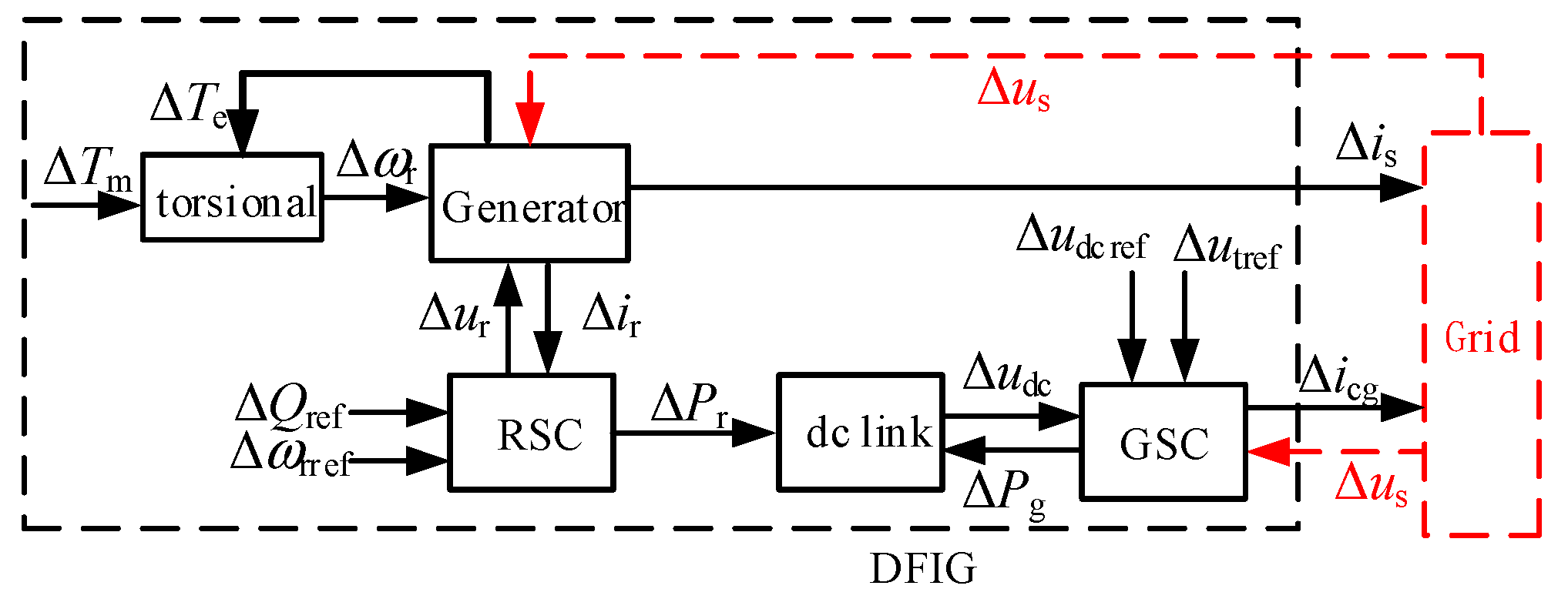
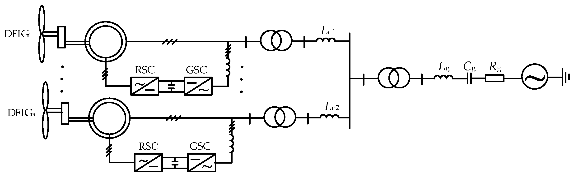
The basic principle of the equivalent model is derived by taking two parallel DFIG turbines connected with series compensated transmission network, in which two DFIG turbines are of the same type, with symmetrical structure, same parameters and load characteristics. The system consists of 3 parts [23]: turbine1, turbine2 of DFIG and grid. The dynamics of each part are given by:

$$\begin{array}{l}{\dot{X}}_{\mathrm{U}1}{=\mathrm{A}}_{\mathrm{U}}{X}_{\mathrm{U}1}+{\mathrm{B}}_{\mathrm{U}}{X}_{\mathrm{L}}\\ {\dot{X}}_{\mathrm{U}2}{=\mathrm{A}}_{\mathrm{U}}{X}_{\mathrm{U}2}+{\mathrm{B}}_{\mathrm{U}}{X}_{\mathrm{L}}\\ {\dot{X}}_{\mathrm{L}}={\mathrm{A}}_{\mathrm{L}}{X}_{\mathrm{L}}+{\mathrm{B}}_{\mathrm{I}}{X}_{\mathrm{U}1}+{\mathrm{B}}_{\mathrm{I}}{X}_{\mathrm{U}2}\end{array}$$

(4)

where state variables subscript 1,2 represents turbine1, turbine2 of DFIG turbine.

The closed-loop system can be described by:

$$\left[\begin{array}{c}{\dot{X}}_{\mathrm{U}1}\\ {\dot{X}}_{\mathrm{U}2}\\ {\dot{X}}_{\mathrm{L}}\end{array}\right]=\left[\begin{array}{ccc}{\mathrm{A}}_{\mathrm{U}}& 0& {\mathrm{B}}_{\mathrm{U}}\\ 0& {\mathrm{A}}_{\mathrm{U}}& {\mathrm{B}}_{\mathrm{U}}\\ {\mathrm{B}}_{\mathrm{I}}& {\mathrm{B}}_{\mathrm{I}}& {\mathrm{A}}_{\mathrm{L}}\end{array}\right]\left[\begin{array}{c}{X}_{\mathrm{U}1}\\ X_{\mathrm{U}2}\\ X_{\mathrm{L}}\end{array}\right]=\mathrm{A}\left[\begin{array}{c}{X}_{\mathrm{U}1}\\ X_{\mathrm{U}2}\\ X_{\mathrm{L}}\end{array}\right].$$

(5)

Based on the similarity transformation theorem that the original matrix and similar matrix have the same eigenvalue, the system state matrix A can be similarly transformed. One of the similar transformation matrix P is:

$$\mathrm{P}=\left[\begin{array}{ccc}{0.5\mathrm{I}}_{\mathrm{U}}& {\mathrm{I}}_{\mathrm{U}}& 0\\ -{0.5\mathrm{I}}_{\mathrm{U}}& {\mathrm{I}}_{\mathrm{U}}& 0\\ 0& 0& {\mathrm{I}}_{\mathrm{L}}\end{array}\right],$$

(6)

where I_U is a 16 × 16 unit matrix, I_L is a 6 × 6 unit matrix. The state matrix A can be diagonalized as B:

$$\mathrm{B}={\mathrm{P}}^{-1}\mathrm{AP}=\left[\begin{array}{ccc}{\mathrm{A}}_{\mathrm{U}}& 0& 0\\ 0& {\mathrm{A}}_{\mathrm{U}}& {\mathrm{B}}_{\mathrm{U}}\\ 0& {2\mathrm{B}}_{\mathrm{I}}& {\mathrm{A}}_{\mathrm{L}}\end{array}\right].$$

(7)

The similarity matrix B is a block diagonal matrix, in which the eigenvalues are the set of two sub-matrices A_U and [A_U, B_U; 2B_I, A_L], then the eigenvalues of the system state matrix A can be characterized by two sub-matrices.

There is no relationship between the eigenvalues of two sub-matrices, which correspond to two separate units. The first part A_U can be called single-machine to infinite bus system, which is equivalent to one DFIG turbine directly connected to an infinite bus. The second part [A_U, B_U; 2B_I, A_L] can be called modified single-machine to the grid, which is equivalent to the current component B_I in the grid interface of a single DFIG turbine multiplied by coefficient 2 and then connected to the infinite system through the original transmission line.

Since the similarity transformation matrix P is not unique, countless similarity transformation matrices can be constructed for the system state matrix A. Further analysis shows that the similarity transformation matrix of matrix A satisfies condition:

• sub-matrix A_U has not changed.
• sub-matrix [A_U, k₁B_U; k₂B_I, A_L] satisfies the product of the coefficient k₁ and k₂ of the current component B_U and voltage component B_I is 2.

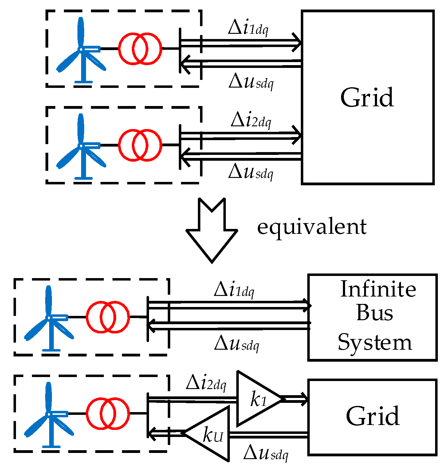
Therefore, the two-machine system can be equivalent, as shown in Figure 4. Among them, single-machine to the infinite bus can reflect the oscillation modes in DFIG turbines, while the modified single-machine to the grid can reflect the oscillation modes between DFIG turbines and the grid. Since it is always stable to single-machine to the infinite bus, the system’s stability under SSR only depends on the single-machine to grid.

4.2. Equivalent Model of the N-Machine System

When n (n > 2) parallel DFIG turbines connected with series compensated transmission network, the equivalent model can be constructed based on the same method. Among them, DFIG turbines are of the same type, in which n parallel DFIG turbines are in the same type, with symmetrical structure, same parameters and load characteristics. The n-machine system state matrix A_N is as follows:

$${\mathrm{A}}_{\mathrm{N}}=\left[\begin{array}{lllll}{\mathrm{A}}_{\mathrm{U}}\hfill & 0\hfill & \cdots \hfill & 0\hfill & {\mathrm{B}}_{\mathrm{U}}\hfill \\ 0\hfill & \ddots \hfill & \hfill & ⋮\hfill & ⋮\hfill \\ ⋮\hfill & \hfill & \ddots \hfill & 0\hfill & ⋮\hfill \\ 0\hfill & \cdots \hfill & 0\hfill & {\mathrm{A}}_{\mathrm{U}}\hfill & {\mathrm{B}}_{\mathrm{U}}\hfill \\ {\mathrm{B}}_{\mathrm{I}}\hfill & \dots \hfill & \dots \hfill & {\mathrm{B}}_{\mathrm{I}}\hfill & {\mathrm{B}}_{\mathrm{U}}\hfill \end{array}\right].$$

(8)

Based on the similarity transformation theorem, matrix A_N can be similarly transformed as:

$${\mathrm{P}}_{\mathrm{N}}{}^{-1}{\mathrm{A}}_{\mathrm{N}}{\mathrm{P}}_{\mathrm{N}}=\left[\begin{array}{lllll}{\mathrm{A}}_{\mathrm{U}}\hfill & 0\hfill & \cdots \hfill & 0\hfill & 0\hfill \\ 0\hfill & \ddots \hfill & \hfill & ⋮\hfill & ⋮\hfill \\ ⋮\hfill & \hfill & \ddots \hfill & 0\hfill & ⋮\hfill \\ 0\hfill & \cdots \hfill & 0\hfill & {\mathrm{A}}_{\mathrm{U}}\hfill & k_1{\mathrm{B}}_{\mathrm{U}}\hfill \\ 0\hfill & \dots \hfill & \dots \hfill & k_2{\mathrm{B}}_{\mathrm{I}}\hfill & {\mathrm{B}}_{\mathrm{U}}\hfill \end{array}\right].$$

(9)

The eigenvalues of n-machine system state matrix A_N can be composed of two parts. The first part diag [A_U, …, A_U] can be equivalent to single DFIG turbine to infinite bus (the multiplier is n-1), reflecting the oscillation modes in DFIG turbines. The second part [A_U, k₁B_U; k₂B_I, A_L] can be equivalent to a modified single DFIG turbine to grid with the product of the coefficient k₁ and k₂ of the current component B_U and voltage component B_I is n, which reflects the oscillation modes between DFIG turbines and grid.

When the DFIG turbines are of the same type, that is, in the same type, with symmetrical structure, same parameters and load characteristics. The equivalent model greatly reduces the system dimension; after equivalence, the system order is reduced from 16 × n + 6 to 16 (single DFIG turbine to the infinite bus) + 22 order (modified single DFIG turbine to the grid).

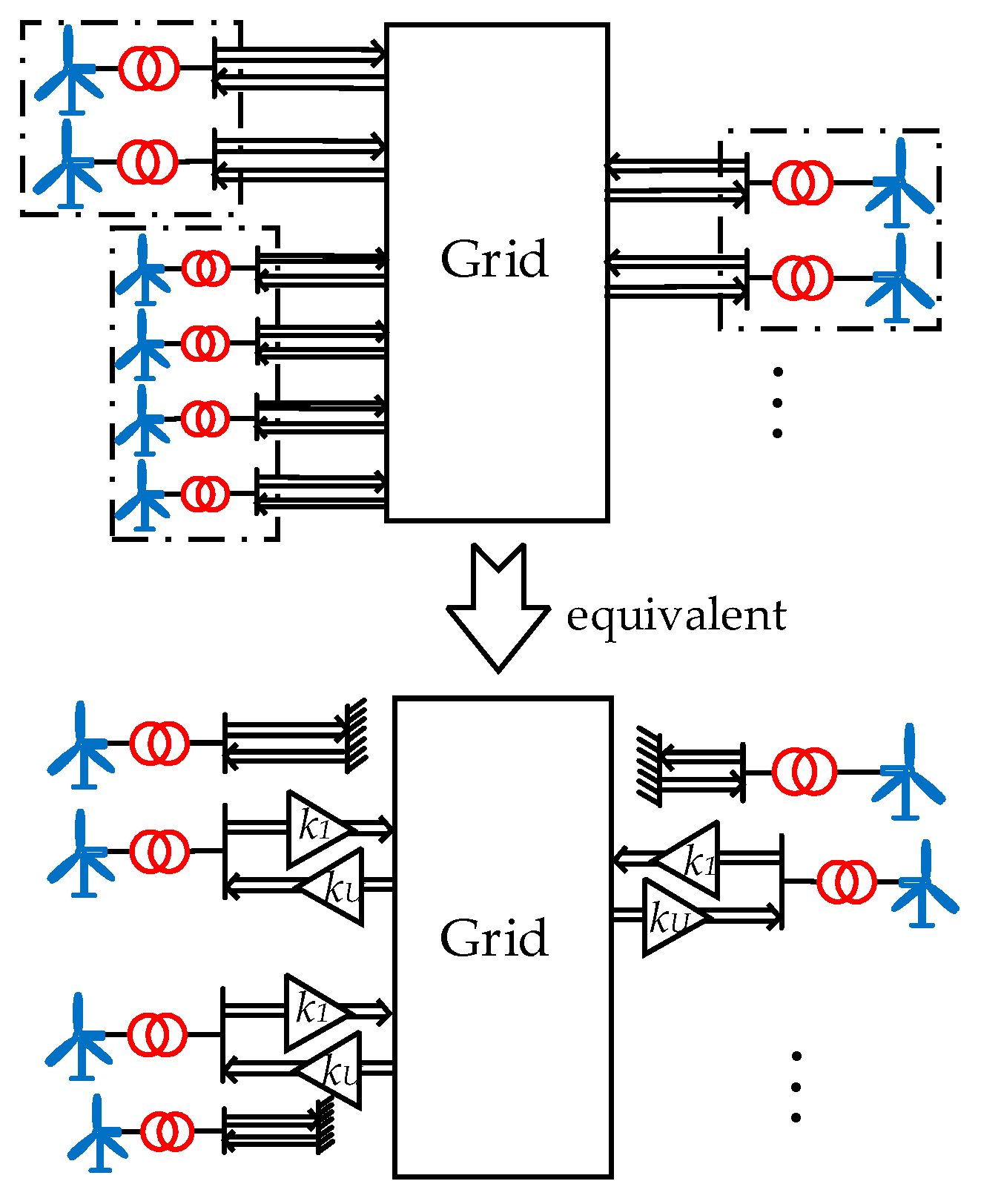
4.3. Equivalent Model of DFIG Wwind Farm

DFIG wind farm consists of hundreds of wind turbines generally. DFIG turbines are difficult to under the same operating conditions due to different position and influence of the wake effect, which cannot meet the equivalent conditions. At this point, DFIG wind farm can be divided into several groups composed of DFIG turbines with similar operating conditions. Hence each group’s DFIG turbines are approximately equivalent to the same operating conditions, each group can be equivalent to two separate units; otherwise, different groups cannot be equivalent. The equivalent model of DFIG wind farm is shown in Figure 5.

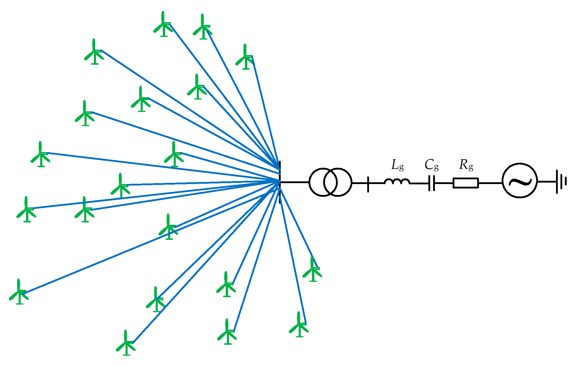
4.4. Wind Farm Equivalence Model Verification

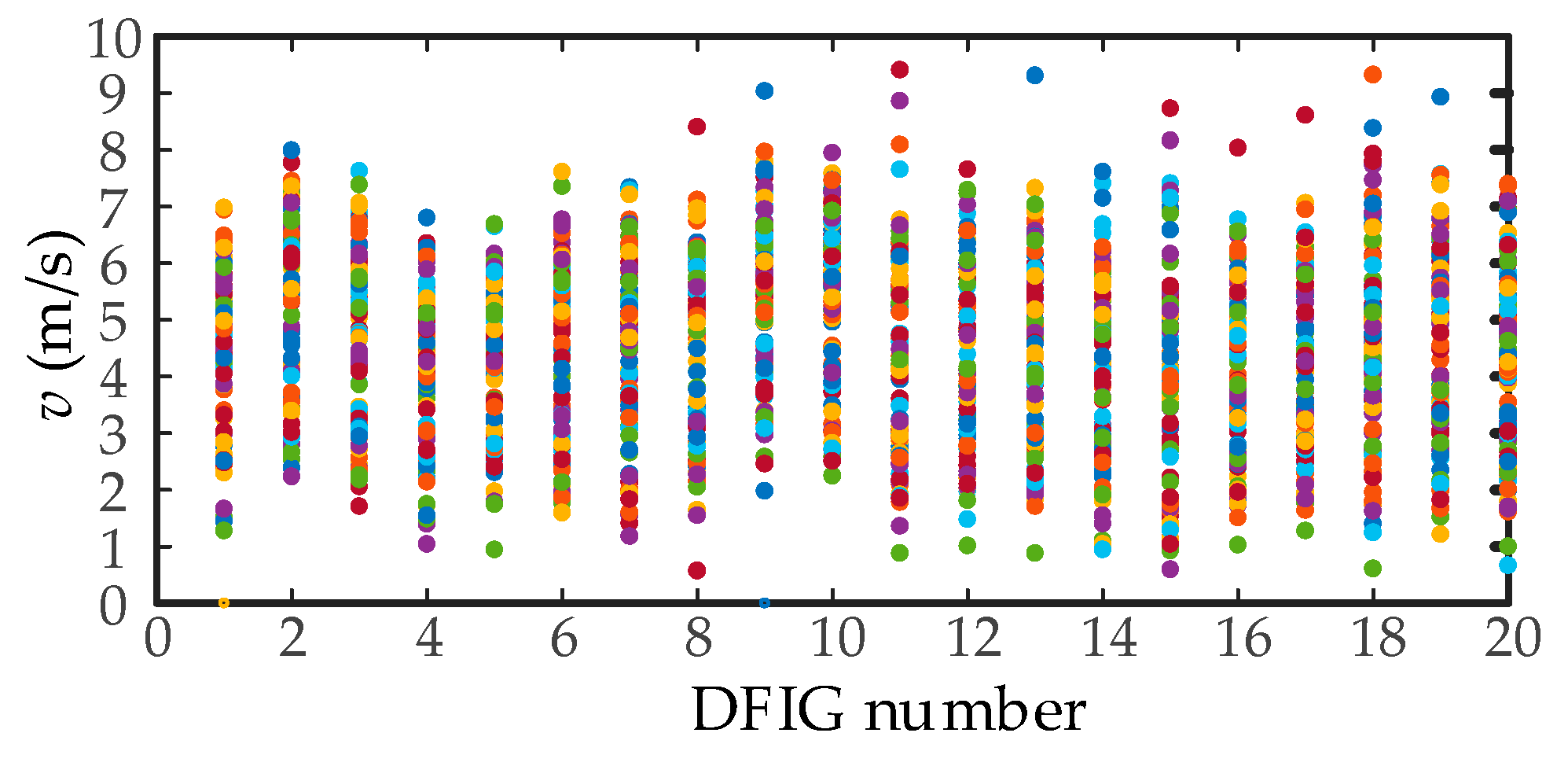
To verify the accuracy of the theoretical analysis, a linearized model of a DFIG wind farm connected with series compensated transmission network as shown in Figure 6 has built, in which DFIG wind farm is characterized by 20 parallel DFIG turbines (the multiplier of each turbine is 100). The 24 h actual wind speed data of 20 wind turbines in a Jilin wind farm is shown in Figure 7 (the sampling interval is 15 min). The actual wind speed data at a certain time t₁ is selected as the input wind speed of DFIG wind farm, as shown in

Table A3. The input wind speed of DFIG wind farm in t₁.

Number	Operating Condition (m/s)	Number	Operating Condition (m/s)
1	5.923	11	4.292
2	6.742	12	4.133
3	5.205	13	4.046
4	5.118	14	3.625
5	5.082	15	3.466
6	5.655	16	3.843
7	5.669	17	3.770
8	6.249	18	5.133
9	6.655	19	3.756
10	6.923	20	4.625

in Appendix B.

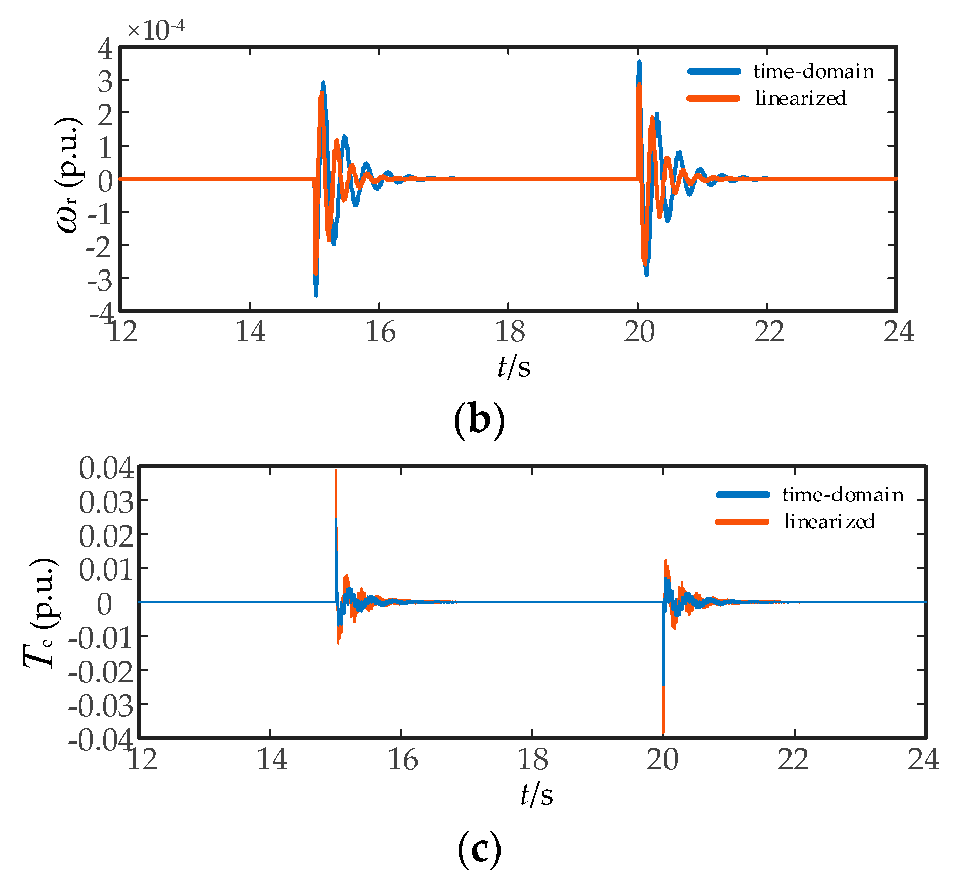
The time domain simulation model and linearized model of detailed DFIG wind farm is constructed, in which the same parameters and operating points are adopted. By setting the DC voltage reference disturbance (t = 15 s, 0.1 p.u. voltage step change is applied; t = 20 s, −0.1 p.u. voltage step change is applied), the matching degree of the results of the two models is compared in Figure 8 to verify the effectiveness of the model.

It can be seen from Figure 8 that after the step disturbance, the time-domain simulation model and the linearized model have the same fluctuation trend of DC voltage u_dc, while the fluctuation amplitude and phase angle of the rotational speed ω_r and the electromagnetic torque T_e are slightly different but the fluctuation trend is roughly the same.

Based on the k-means grouping algorithm [24], determine the number of groups k = 4, the 20 DFIG turbines is divided into 4 groups. The results are shown in

Table 1. The results of grouping.

Groups	Operating Condition (m/s)	Groups	Operating Condition (m/s)
Group 1	3.466		5.118
	3.625		5.133
	3.756		5.205
	3.770	Group 3	5.655
	3.843		5.669
	4.046		5.923
	4.133		6.249
	4.292	Group 4	6.655
Group 2	4.625		6.742
	5.082		6.923

.

Construct a linearized model of the equivalent system and verify the equivalent model’s accuracy, when RSC current inner loop control parameters k_P = 0.01 p.u., the partial eigenvalues of the detailed model and equivalent model are shown in

Table 2. The partial eigenvalues of the detailed model.

Eigenvalues	Frequency	Eigenvalues	Frequency
−5020	0	−11.8	0
−4740	0	−11	0
−4620	0	−8.75 ± j23.5	3.74
−4530	0	−1.9 ± j313	49.84
−4060 ± j17,500	2786.62	−11.1 ± j313	49.84
−1590 ± j15,900	2531.85	−9.78 ± j313	49.84
−111	0	−9.38 ± j313	49.84
−95.9	0	−8.17 ± j313	49.84
−30.6	0	−8.06 ± j313	49.84
−29.4	0	−7.61 ± j371	59.08
−28.6	0	−4.33	0
−27	0	−3.55 ± j3.05	0.49
−26.5	0	−3.48 ± j3.04	0.48
−20.1	0	−3.24 ± j3.03	0.48
−20	0	−3.03 ± j3.02	0.47
−15.9 ± j22.3	3.55	−2.93 ± j258	41.08
−15.9 ± j22.4	3.57	−2.69 ± j3.82	0.61
−15.3 ± j25.2	4.01	−1.33 ± j1.49	0.24
−14.7 ± j27.6	4.39	−1.32 ± j1.50	0.24
−14.2 ± j30.5	4.86	−1.32 ± j1.46	0.23
−14 ± j31.4	5

,

Table 3. The eigenvalues of the modified single-machine to the grid.

Eigenvalues	Frequency	Eigenvalues	Frequency
−5020	0	−14.9 ± j25.1	4.01
−4740	0	−14.1 ± j31.4	5
−4620	0	−11.8	0
−4530	0	−11	0
−4060 ± j17,500	2786.62	−8.98 ± j23.5	3.74
−1590 ± j15,900	2531.85	−11.1 ± j313	49.84
−111	0	−9.28 ± j313	49.84
−95.7	0	−7.61 ± j370	58.92
−30.6	0	−4.35	0
−29.3	0	−3.51 ± j3.06	0.49
−27	0	−3.21 ± j3.04	0.48
−26.3	0	−3.03 ± j3.02	0.47
−20.1	0	−2.91 ± j258	41.08
−20	0	−2.69 ± j3.81	0.61
−15.9 ± j22.1	3.52	−1.31 ± j1.49	0.24
−16 ± j22.4	3.57	−1.32 ± j1.50	0.24
−15.1 ± j27.2	4.33	−1.29 ± j1.45	0.23

and

Table 4. The eigenvalues of the single-machine to an infinite bus.

Eigenvalues	Frequency	Eigenvalues	Frequency
−4740	0	−11	0
−4620	0	−9.83 ± j313	49.84
−111	0	−8.11 ± j313	49.84
−30.6	0	−8.09 ± j313	49.84
−28.6	0	−3.49 ± j3.04	0.48
−26.3	0	−3.24 ± j3.03	0.48
−20.1	0	−3.03 ± j3.02	0.47
−20	0	−3.03 ± j3.02	0.47
−16 ± j22.6	3.60	−1.32 ± j1.50	0.24
−15.9 ± j22.1	3.52	−1.31 ± j1.47	0.23
−15.1 ± j27.1	4.32	−1.31 ± j1.49	0.24
−14.2 ± j32	5.10	−1.29 ± j1.45	0.23
−11.7 ± j313	49.84

.

According to Table 2, Table 3 and Table 4, when k_P = 0.01 p.u., the system is stable, the error rate of the real part of the eigenvalues by the equivalent model is less than 2.7% and that of the imaginary part is less than 1.5%, in which the real part error rate of dominant oscillation eigenvalues is 0.68% and there is no error in the imaginary part.

To avoid the influence of chance on the accuracy of the equivalent model, when actual wind speed data at a certain time t₂ is selected as the input wind speed of DFIG wind farm, the input wind speed and grouping results are shown in

Table A4. The input wind speed of DFIG wind farm in t₂.

Number	Operating Condition (m/s)	Number	Operating Condition (m/s)
1	4.611	11	4.727
2	6.162	12	4.785
3	5.118	13	4.596
4	4.335	14	5.582
5	4.357	15	3.93
6	4.335	16	4.364
7	5.698	17	4.698
8	5.249	18	4.77
9	5.684	19	4.292
10	6.119	20	4.002

and

Table A5. The results of grouping in t₂.

Groups	Operating Condition (m/s)	Sub-Groups	Operating Condition (m/s)
Group 1	3.93		4.727
	4.002		4.77
	4.292		4.785
	4.335	Group 3	5.118
	4.335		5.249
	4.357	Group 4	5.692
	4.364		5.684
Group 2	4.596		5.582
	4.611	Group 5	6.119
	4.698		6.162

in Appendix B. When RSC current inner loop control parameters k_P = 0.01 p.u., the partial eigenvalues of the detailed and equivalent models are shown in

Table A6. The partial eigenvalues of detailed model and equivalent model.

Detailed Model	Single-Machine to Infinite Bus System	Modified Single-Machine to Grid System
−5020	−4960
−4740	−4740	−4740
−4620	−4620	−4620
−4530	−4590
−4010 ± j17,400	−4000 ± j17,400
−1570 ± j15,800	−1590 ± j15,800
−111	−111	−111
−93	−92.6
−30.7	−30.7	−30.7
−30.6		−30.6
−30.2	−30.3
−29.5	−29.4
−29		−29.1
−28.2	−28.2
−27.9		−27.9
−20.1	−20.1	−20.1
−20	−20	−20
−16 ± j22.2	−16 ± j22.2
−16 ± j22		−16 ± j22
−15.8 ± j23.4	−15.8 ± j23.1	−15.8 ± j23.3
−15.3 ± j25.6		−15.4 ± j25.9
−15.3 ± j24.8	−15.3 ± j24.9
−14.8 ± j28.3	−14.8 ± j27.8	−14.9 ± j28.5
−14.7	−14.7
−11.9	−11.9
−11	−11	−11
−10.4 ± j313		−10.4 ± j313
−10.1 ± j313	−10.1 ± j313
−9.32 ± j313		−9.36 ± j313
−9.07 ± j313	−9.1 ± j313
−8.96 ± j23	−8.92 ± j23.1
−8.5 ± j313		−8.4 ± j313
−8.25 ± j313	−8.35 ± j313
−8.06 ± j313	−8.06 ± j313	−8.06 ± 313
−7.62 ± j370	−7.62 ± j370
−4.21	−4.2
−3.31 ± j3.04	−3.3 ± j3.03
−3.18 ± j3.03		−3.18 ± j3.03
−3.15 ± j3.03	−3.16 ± j3.03
−3.08 ± j3.02	−3.06 ± j3.02	−3.07 ± j3.02
−3.03 ± j3.02	−3.03 ± j3.02	−3.03 ± j3.02
−2.63 ± j3.84	−2.62 ± j3.85
−2.46 ± j259	−2.45 ± j259
−1.32 ± j1.50	−1.32 ± j1.50	−1.32 ± j1.50
−1.31 ± j1.46	−1.31 ± j1.46	−1.31 ± j1.46

in Appendix B. According to Table A6, when k_P = 0.01, the system is stable, the error rate of the real part of the eigenvalues by the equivalent model is less than 1.3% and that of imaginary part is less than 1.8%, in which the real part error rate of dominant oscillation eigenvalues is 0.41% and there is no error in the imaginary part.

To sum up, under the two example conditions: the error rate of the real part of the equivalent model eigenvalues is less than 2.7% and that of the imaginary part is less than 1.8%, in which the real part error rate of dominant oscillation eigenvalues is less than 0.68% and there is no error in imaginary part. Otherwise, the time-domain simulation time of the detailed model is 96 min and that of the equivalent model is 3 min. The equivalent model simulation time is greatly shortened.

5. Validity Analysis of the Equivalent Model

When actual wind speed data at a certain time t₁ is selected as the input wind speed of DFIG wind farm, the validity of the equivalent model under SSR is analyzed when the number of DFIG turbines and the length of collecting lines are different. At the same time, other influencing factors, such as the RSC tie-reactor, on the accuracy of the equivalent model are also studied. In addition, the applicability of the equivalent model to super-synchronous oscillation is briefly analyzed.

The average Euclidean distance is introduced as the evaluation index:

$$d=\frac{1}{n}{\displaystyle \sum _{i=1}^n\sqrt{{\left[\mathrm{Re}\left({\lambda }_{\mathrm{e}}\right)-\mathrm{Re}\left({\lambda }_{\mathrm{i}}\right)\right]}^2+{\left[\mathrm{Im}\left({\lambda }_{\mathrm{e}}\right)-\mathrm{Im}\left({\lambda }_{\mathrm{i}}\right)\right]}^2}}$$

(10)

where λ_e and λ_i are the dominant oscillation eigenvalues of the equivalent model and the detailed model respectively; n is the number of dominant oscillation eigenvalues. The smaller the average Euclidean distance, the more accurately the equivalent model can express the dominant oscillation characteristics.

5.1. When the Difference in Collecting Lines and DFIG Turbines Number Is Not Considered

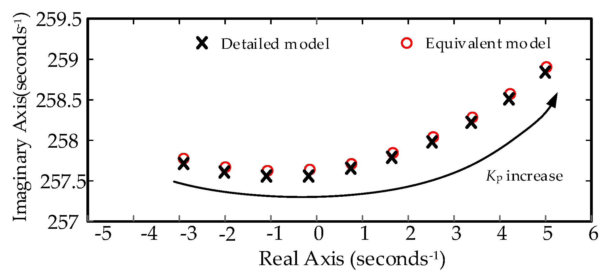
Case 1: 20 DFIG turbines have the same number (the multiplier of each turbine is 100) and the collecting lines are not considered, the validity of the equivalent model under SSR is analyzed by changing the RSC current inner loop control parameter k_P. When k_P is between 0.01 p.u. to 0.1 p.u., the results of dominant oscillation eigenvalues of the detailed model and equivalent model are shown in Figure 9.

It can be seen from Figure 9 that when k_P changes from 0.01 p.u. to 0.1 p.u., the variation trend in equivalent model is the same as that in detailed model, in which the average Eucalyptus distance of the dominant eigenvalues is between 0.02 p.u. to 0.03 p.u. In this case, the equivalent model can accurately reflect the dominant oscillation characteristics of the DFIG wind farm and effectively reduce the dimension.

5.2. When the Difference of DFIG Turbines Number Is Considered

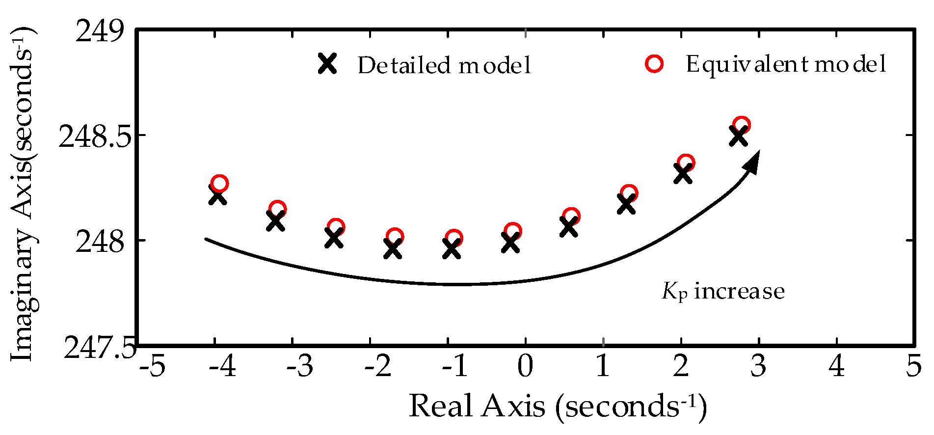
Case 2: Set the number of i-th wind turbines is 100 + 10(i-1) and the collecting lines is not considered. When k_P is between 0.01 p.u. to 0.1 p.u., the results of dominant oscillation eigenvalues of detailed model and equivalent model are shown in Figure 10.

It can be seen from Figure 10 that when k_P changes from 0.01 p.u. to 0.1 p.u., the variation trend in equivalent model is the same as that in detailed model, in which the average Eucalyptus distance of the dominant eigenvalues is between 0.03 p.u. to 0.04 p.u., When considering the difference in the number of DFIG turbines, the accuracy of the dominant oscillation eigenvalues of the equivalent model is basically unchanged.

5.3. When the Difference of Collecting Lines Is Considered

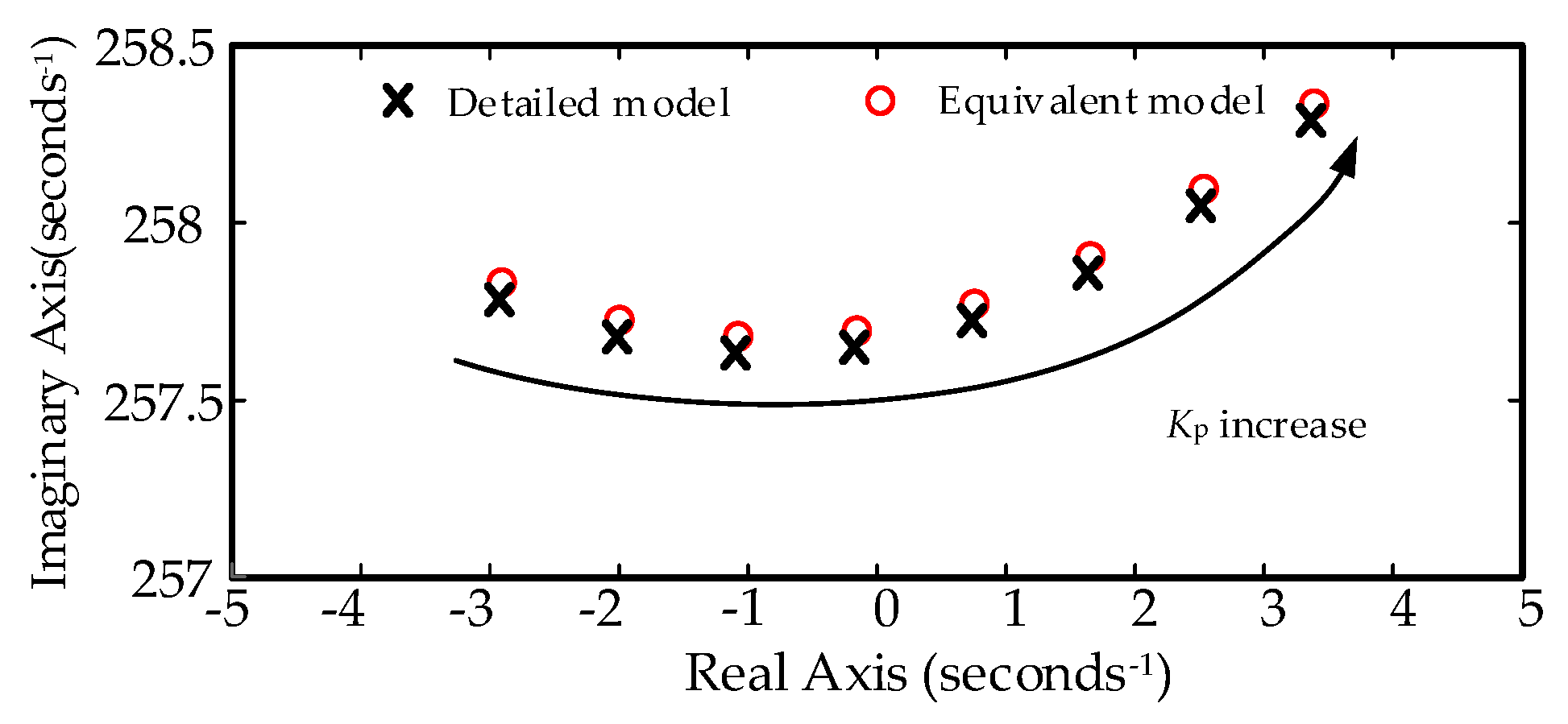
Case 3: For the i-th DFIG turbine, the collecting line’s length is set to be 0.5 + 0.01 (i-1) km and the number is the same (the multiplier of each turbine is 100). The equivalent model’s collection line adopts the power loss equivalent method, that is, the original network is replaced with an equivalent impedance [25], so that the loss of the equivalent model output power at the equivalent impedance is equal to that of before the equivalent. The power loss on the collector network remains consistent. When k_P is between 0.01 p.u. to 0.1 p.u., the results of dominant oscillation eigenvalues of detailed model and equivalent model are shown in Figure 11.

It can be seen from Figure 11 that when k_P changes from 0.01 p.u. to 0.1 p.u., the variation trend in equivalent model is the same as that in detailed model, in which the average Eucalyptus distance of the dominant eigenvalues is between 0.02 p.u. to 0.03 p.u. When considering the difference of the collecting lines, the accuracy of the dominant oscillation eigenvalues of the equivalent model is basically unchanged.

5.4. Influence of RSC Connection Inductance

According to Reference [26], the RSC tie-reactor may affect the oscillation characteristics of DFIG model. Based on the linearized model, the influence of RSC tie-reactor is studied. When RSC connecting inductance L_rsc changes, the eigenvalues of the detailed model and the equivalent model are as follows.

As can be seen from

Table 5. The eigenvalues of detailed model and equivalent model when L_rsc changes.

Change of Lrsc	Detailed Model	Equivalent Model
−0.03 p.u.	−2.99 ± j258	−2.97 ± j258
−0.02 p.u.	−2.97 ± j258	−2.95 ± j258
−0.01 p.u.	−2.95 ± j258	−2.93 ± j258
0	−2.93 ± j258	−2.91 ± j258
0.01 p.u.	−2.91 ± j258	−2.89 ± j258
0.02 p.u.	−2.90 ± j258	−2.87 ± j258
0.03 p.u.	−2.89 ± j258	−2.86 ± j258

, with the change of L_rsc, the eigenvalues of the detailed model and the equivalent model also change. Therefore, the value of RSC tie-reactor should be set as accurate as possible during modeling, so as to improve the accuracy of the model.

5.5. Applicability of Equivalent Model for Super-Synchronous Oscillation

According to the eigenvalues results of Table 2, Table 3 and Table 4 in Section 4.4, there is a pair of conjugate eigenvalues in super-synchronous range in the detailed model and the equivalent model. Set the proportional coefficient k_P in the inner ring of RSC from 0.01 p.u. to 0.1 p.u., the effect of the equivalent model on the super-synchronous oscillation is studied. The dominant eigenvalues of the super-synchronous oscillation are as follows.

It can be seen from

Table 6. The eigenvalues of super-synchronous oscillation.

Kp	Detailed Model	Frequency	Single-Machine to Infinite Bus System	Frequency
0.01	−7.61 ± j371	59.36	−7.61 ± j370	58.92
0.02	−8.24 ± j370	58.92	−8.24 ± j370	58.92
0.03	−8.86 ± j370	58.92	−8.87 ± j370	58.92
0.04	−9.48 ± j370	58.92	−9.48 ± j370	58.92
0.05	−10.1 ± j370	58.92	−10.1 ± j370	58.92
0.06	−10.7 ± j370	58.92	−10.7 ± j370	58.92
0.07	−11.3 ± j369	58.92	−11.3 ± j369	58.92
0.08	−11.9 ± j369	58.76	−11.9 ± j369	58.76
0.09	−12.4 ± j369	58.76	−12.4 ± j369	58.76
0.10	−13.0 ± j368	58.60	−13.0 ± j368	58.60

that the system’s super-synchronous oscillation is not excited under the current case conditions. When k_P changes, the equivalent model can accurately reflect the change trend of the eigenvalues of the detailed model, the error rate of real part of eigenvalues by equivalent model is less than 0.11% and that of imaginary part is less than 0.77%.

6. Damping Analysis

The detailed model and equivalent model of DFIG wind farm connected with series compensated transmission network are built in EMTDC/PSCAD. The DFIG turbine parameter is shown in

Table A7. Parameter of DFIG.

Parameter	Unit/p.u.
Stator resistance rs	0.0164
Stator leakage reactance Xs	0.255
Rotor resistance rr	0.0183
Rotor leakage reactance Xr	0.222
Excitation reactance Xm	13.68

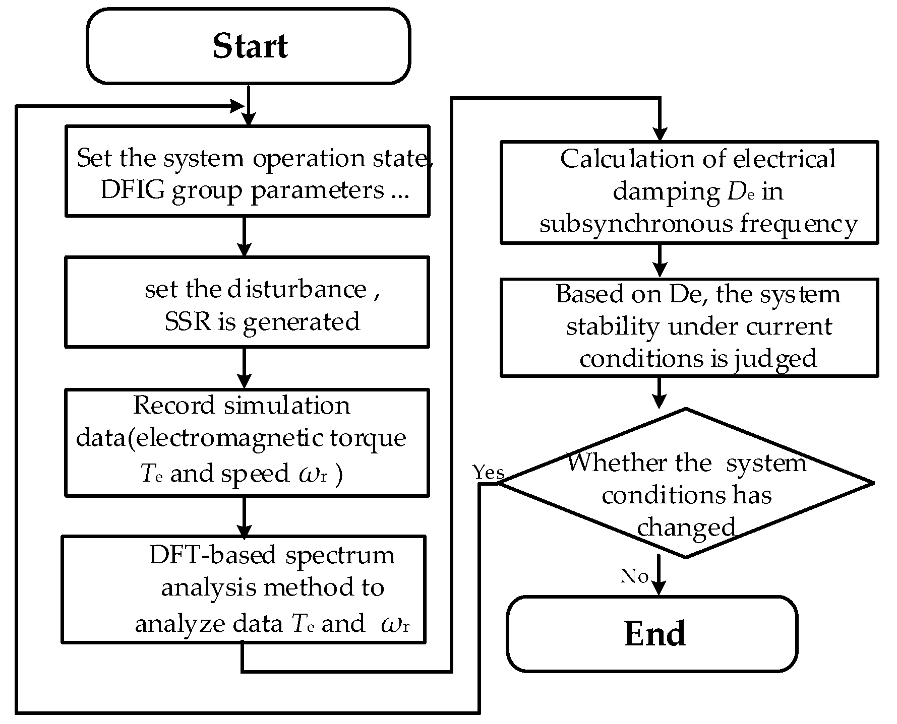
in Appendix B and the series of compensation degrees of the system is 6.67%. Based on the damping analysis method, the equivalent model’s effectiveness is further verified and the oscillation mechanism is further revealed. The flowchart of online damping analysis is shown in Figure 12.

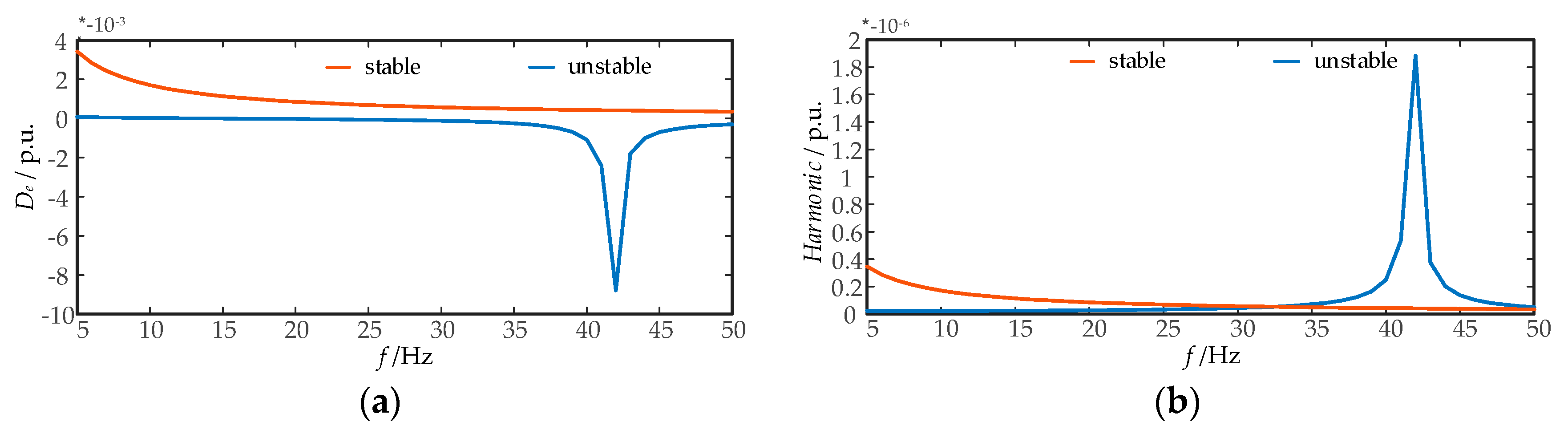
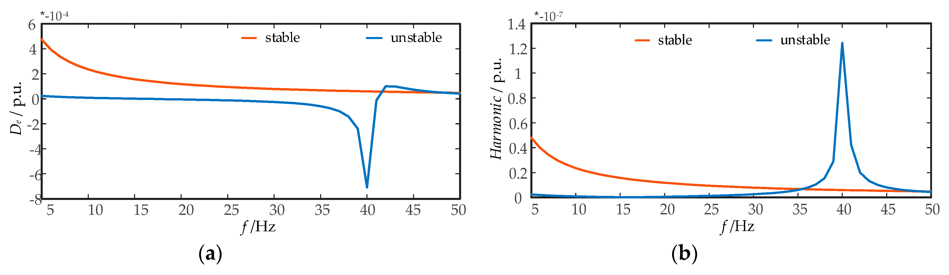
Under the conditions of case 1 and case 2, when it occurs to SSR, the electrical damping coefficient D_e and the inter-harmonic distribution in the electromagnetic torque of one of the DFIG turbines in the equivalent model are shown in Figure 13 and Figure 14.

According to Figure 13 and Figure 14, it can be seen that: under the condition of case 1, when the system is stable, the electromagnetic damping coefficient D_e of DFIG turbine is always positive and there is no harmonic; when the system is unstable, the oscillation frequency is about 42 Hz in case 1 (40 Hz in case 2) which is consistent with the result of eigenvalue analysis. When f = 42 Hz in case 1 (40 Hz in case 2), the electromagnetic damping coefficient D_e of DFIG turbine becomes negative, which leads to oscillation instability of the system.

7. Conclusions

Based on the principle that the similarity matrix has the same eigenvalues, the equivalence of DFIG wind farm connected with the series compensated transmission network has been studied and the equivalence process has a strict theoretical basis. Then, through the eigenvalue analysis method, the effectiveness of DFIG wind farm’s equivalent model is analyzed considering the differences in the number of DFIG turbines and the collection lines. Finally, a simulation model is built in EMTDC/PSCAD, through the online damping analysis method, the equivalent model’s effectiveness is further verified and the oscillation mechanism is further revealed. The results show that:

The same parallel DFIG wind turbines connected with series compensated transmission network can be characterized by two separate units. One unit can reflect the oscillation model between DFIG turbines and the other one can reflect the oscillation model between DFIG turbines and grid. As for DFIG wind turbines which do not meet the equivalence conditions, based on the similarity of operational conditions. Thence, DFIG wind farm is divided into groups and each group can be equivalent to two separate units, while different groups cannot be equivalent.

The equivalent model can accurately reflect the dominant oscillation characteristics of DFIG wind farm. The average Euclidean distance of dominant eigenvalues is about 0.02~0.03. When considering the difference between the number of DFIG turbines and the collector lines, the accuracy of the equivalent model is basically unchanged. In addition, the equivalent model can reflect the super-synchronous oscillation characteristics.

Based on the online damping analysis method, the mechanism of SSR in DFIG wind farm connected with series compensated transmission network is explained. When the system oscillates, the electromagnetic damping coefficient of DFIG turbines are negative. Under the oscillation frequency, the system damping becomes smaller which leads the system unstable.