A Comparative Analysis of Neutron Transport Calculations Based on Variational Formulation and Finite Element Approaches

Abstract

The application of continuous and discontinuous approaches of the finite element method (FEM) to the neutron transport equation (NTE) has been investigated. A comparative algorithm for analyzing the capability of various types of numerical solutions to the NTE based on variational formulation and discontinuous finite element method (DFEM) has been developed. The developed module is coupled to the program discontinuous finite element method for neutron (DISFENT). Each variational principle (VP) is applied to an example with drastic changes in the distribution of neutron flux density, and the obtained results of the continuous and discontinuous finite element (DFE) have been compared. The comparison between the level of accuracy of each approach using new module of DISFENT program has been performed based on the fine mesh solutions of the multi-PN (MPN) approximation. The obtained results of conjoint principles (CPs) have been demonstrated to be very accurate in comparison to other VPs. The reduction in the number of required meshes for solving the problem is considered as the main advantage of this principle. Finally, the spatial additivity to the context of the spherical harmonics has been implemented to the CP, to avoid from computational error accumulation.

1. Introduction

The Boltzmann equation describes the local density of particles traveling inside a medium with interactions between the particles and the medium, involving the independent variables of position, time, energy, and direction of motion. Applying the well-known approaches to handle the spatial dependence of this equation is one of the central problems of nuclear reactor theory. Among these approaches, the finite element (FE), finite difference, and nodal methods are considered as the most efficient approaches [1,2,3,4,5]. The FE approach as a computer-based method can be applied for numerically solving a wide range of boundary value problems. In recent decades, there has been an increasing tendency in analyzing the neutronic aspects of the reactor, especially numerical solution of neutron transport equation (NTE), to employ techniques based on the families of discontinuous and continuous Galerkin finite element methods (FEMs). The discontinuous finite element (DFE) procedure makes use of the same function space as the continuous procedure, but with relaxed continuity at interface boundaries of each element or each region [6]. It was first introduced by Reed and Hill for the solution of the NTE [7], and recent developments have been reviewed by [8,9]. The essential idea of discontinuous finite element method (DFEM) is derived from the fact that the shape functions can be chosen so that either the field variable or its derivatives, or generally both, are considered discontinuous across the interfaces of elements, while the computational domain continuity is maintained. As a result, the DFEM includes, as its subset, both the FEM and the finite difference method. Therefore, it has the advantages of both the finite difference and the FEMs, in that it can be effectively used in generating various types of meshes with maintaining geometric flexibility and controlling the order of angular approximations through each element. This feature makes it uniquely useful for computational neutron transport calculations. Because of the local nature of a discontinuous formulation, unlike the continuous methods, no global matrix (GM) needs to be assembled; and thus, this reduces the demand on the memory. The effects of the boundary conditions on the interior field distributions then gradually propagate through element-by-element connection. This is another important feature that makes this method useful for neutron transport calculations.

In comparison with the other numerical methods (finite difference and FEs), the discontinuous FE plan has both advantages and disadvantages, which are important for developing specific applications [10,11].

The scalar flux often has a changeable and unstable treatment in different regions with respect to the physical conditions of the system. For example in cases, where the absorption cross-section has a high value, encountering very strong gradients in the scalar flux and discontinuity in angular flux (AF) at interfaces is predictable. This discontinuity mostly can be found in some problems with rapid changes in scalar flux. Therefore, the DFEM can improve these depletions, easily. In addition, the coupling between element variables is achieved through the boundary integrals only. This means that the source terms and stiffness matrixes are fully decoupled between elements, and some special techniques are applied to assembling the local matrixes. With the use of these techniques and considering no dependence between elements, one can find that the order of angular approximation is changeable for each element with respect to the necessity of the problem. Hence, a DFE algorithm will not result in an assembled GM, and thus, the in-core memory demand is not as strong. Furthermore employing the DFEM leads to decreasing the cost of the calculations, while the values of errors are decreasing. In addition, the local formulation makes it very easy and comfortable to parallelize the algorithm, taking advantage of either shared memory parallel computing or distributed parallel computing, which is not the purpose of this paper. Finally, because of the local formulation, both the $h$-adaptive (mesh size optimization) and $p$-adaptive (optimization the order of angular approximations) refinements are made convenient. The $hp$-adaptive algorithm (mesh and order of angular approximation optimization) based on the discontinuous formulation requires no additional cost associated with node renumbering compared with the continuous finite element (CFE) method. Various approaches have been adapted to interpret the concept of discontinuous and two widely accepted ones, which are based on variational methods in comparison to the CFE method are presented in this paper [12,13,14,15,16].

FEMs (both continuous and discontinuous) have been applied by various techniques to solve NTE. In some techniques, a weighted residual approach is used, while in others, the variational methods are used. In 1997, the classical maximum principle-based on a generalized least-square approach to obtain CFE solutions of the even-parity transport equation (TE) was presented by Ackroyd [17]. The application of variational approaches for solving the NTE has been investigated over recent years.

The numerical solutions to the NTE based on variational formulation and continuous/discontinuous FEM have been successfully applied to our previous investigations: In 2011 an adaptive CFE approach for NTE was applied by Abbasi et al. [18]. As the second study of our group, the spatially adaptive hp refinement approach for the PN NTE using the spectral element method based on the CFE method was carried out [19]. In 2018, an extended half-range spherical harmonics method for first-order NTE based on variational treatment and CFE was presented by Ghazaie et al. [20,21]. In 2019, Yousefi et al. [22] performed an investigation for CFE modeling of the 3D NTE based on the variational methods, and the computational program ENTRANS was developed. Finally, in 2018, Sadeghi et al. [23] applied an adaptive refinement for the PN NTE based on conjoint variational formulation, and DFEM and the new computer code, discontinuous finite element method for neutron transport (DISFENT), in two-dimensional geometry was developed. The main goal of this study is to present a comparative analysis of numerical neutron transport calculations using the variational formulation based on the continuous and discontinuous FEMs. This paper is organized as follows: The theoretical background of the NTE based on even and odd components is presented in the next section. Developing the variational principles (VPs) by considering the direction of motion and spatial dependence to NTE is analyzed in the third section. In Section 3, the maximization of the VP based on changing the penalty parameter is performed. Developing the formulation of the DFE with the element by element neutron conservation (NC) and conjoint maximization is presented in Section 3.

Finally, in Section 4, to compare the performance of both continuous and DFE approaches that are reviewed in the article, each VP is applied to the well-known Reed’s edge cell [24] benchmark problem. In order to achieve this goal, the developed computer code DISFENT, in which the module of performing the calculation based on the CFE is also added, has been applied.

2. Theoretical Background

The full NTE is an integro-differential equation in seven independent variables (three in space, two in angle, one in energy, and one in time), and as a consequence, the number of degrees of freedom that would be required, for the accurate discretization of all the independent variables can grow extremely quickly. However, the monoenergetic approximation, called one-speed approximation, which is most widely considered neutron transport model both analytically and numerically, is described as [25]:

$$\overrightarrow{\mathsf{\Omega }}.\overrightarrow{\mathit{\nabla }}{\phi }_0\left(\overrightarrow{r},\overrightarrow{\mathsf{\Omega }}\right)+{\sigma }_t\left(\overrightarrow{r}\right){\phi }_0\left(\overrightarrow{r},\overrightarrow{\mathsf{\Omega }}\right)=\underset{4\pi }{{\displaystyle \int }}d{\mathsf{\Omega }}^{\prime }{\sigma }_s\left(\overrightarrow{r},\overrightarrow{\mathsf{\Omega }}.{\mathsf{\Omega }}^{\prime }\right){\phi }_0\left(\overrightarrow{r},{\overrightarrow{\mathsf{\Omega }}}^{\prime }\right)+Q\left(\overrightarrow{r},\overrightarrow{\mathsf{\Omega }}\right)$$

(1)

where $Q\left(\overrightarrow{r},\overrightarrow{\mathsf{\Omega }}\right)$ is the distributed extension source of the neutron, ${\sigma }_t$($\overrightarrow{r}$) is the total cross-section, and ${\sigma }_{\mathrm{s}}\left(\overrightarrow{r},\overrightarrow{\mathsf{\Omega }}.{\overrightarrow{\mathsf{\Omega }}}^{\prime }\right)$ is the differential scattering cross-section at $\overrightarrow{r}$ for scattering from the direction ${\overrightarrow{\mathsf{\Omega }}}^{\prime }$ into the direction $\overrightarrow{\mathsf{\Omega }}$.

Equation (1) is the first order form of NTE in its steady-state formulation. However, for generating the VPs, the second-order of TE is required [17]. Hence, the even and odd parity (EAOP) TE is derived.

EAOP Transport Equation

The second-order forms of the TE are obtained by splitting the components of this equation into the EAOP. According to this, the EAOP of AF can be expressed as:

$${\phi }^{+}\left(\overrightarrow{r},\overrightarrow{\mathsf{\Omega }}\right)=\frac{1}{2}\left[\phi \left(\overrightarrow{r},\overrightarrow{\mathsf{\Omega }}\right)+\phi \left(\overrightarrow{r},-\overrightarrow{\mathsf{\Omega }}\right)\right]$$

(2)

$${\phi }^{-}\left(\overrightarrow{r},\overrightarrow{\mathsf{\Omega }}\right)=\frac{1}{2}\left[\phi \left(\overrightarrow{r},\overrightarrow{\mathsf{\Omega }}\right)-\phi \left(\overrightarrow{r},-\overrightarrow{\mathsf{\Omega }}\right)\right]$$

(3)

This definition can be developed for neutron source and cross-sections too:

$$Q^{+}\left(\overrightarrow{r},\overrightarrow{\mathsf{\Omega }}\right)=\frac{1}{2}\left[Q\left(\overrightarrow{r},\overrightarrow{\mathsf{\Omega }}\right)+Q\left(\overrightarrow{r},-\overrightarrow{\mathsf{\Omega }}\right)\right]$$

(4)

$$Q^{-}\left(\overrightarrow{r},\overrightarrow{\mathsf{\Omega }}\right)=\frac{1}{2}\left[Q\left(\overrightarrow{r},\overrightarrow{\mathsf{\Omega }}\right)-Q\left(\overrightarrow{r},-\overrightarrow{\mathsf{\Omega }}\right)\right]$$

(5)

$${\Sigma }_s{}^{+}\left(\overrightarrow{r},\overrightarrow{\mathsf{\Omega }}.{\overrightarrow{\mathsf{\Omega }}}^{\prime }\right)=\frac{1}{2}\left[{\Sigma }_s\left(\overrightarrow{r},\overrightarrow{\mathsf{\Omega }},{\overrightarrow{\mathsf{\Omega }}}^{\prime }\right)+{\Sigma }_s\left(\overrightarrow{r},-\overrightarrow{\mathsf{\Omega }},{\overrightarrow{\mathsf{\Omega }}}^{\prime }\right)\right]$$

(6)

From the above definitions, it is found:

$${\Sigma }_s{}^{-}\left(\overrightarrow{r},\overrightarrow{\mathsf{\Omega }}.{\overrightarrow{\mathsf{\Omega }}}^{\prime }\right)=\frac{1}{2}\left[{\Sigma }_s\left(\overrightarrow{r},\overrightarrow{\mathsf{\Omega }},{\overrightarrow{\mathsf{\Omega }}}^{\prime }\right)-{\Sigma }_s\left(\overrightarrow{r},-\overrightarrow{\mathsf{\Omega }},{\overrightarrow{\mathsf{\Omega }}}^{\prime }\right)\right]$$

(7)

$${\phi }_0\left(\overrightarrow{r},\overrightarrow{\mathsf{\Omega }}\right)={\phi }_0{}^{+}\left(\overrightarrow{r},\overrightarrow{\mathsf{\Omega }}\right)+{\phi }_0{}^{-}\left(\overrightarrow{r},\overrightarrow{\mathsf{\Omega }}\right).$$

(8)

Now, these parity fluxes and sources are substituted into Equation (1) to obtain the mixed parity equations:

$$\overrightarrow{\mathsf{\Omega }}.\overrightarrow{\nabla }{\phi }^{-}{}_0\left(\overrightarrow{r},\overrightarrow{\mathsf{\Omega }}\right)+\mathrm{C}{\phi }^{+}{}_0\left(\overrightarrow{r},\overrightarrow{\mathsf{\Omega }}\right)=Q^{+}\left(\overrightarrow{r},\overrightarrow{\mathsf{\Omega }}\right)$$

(9)

$$\overrightarrow{\mathsf{\Omega }}.\overrightarrow{\nabla }{\phi }^{+}{}_0\left(\overrightarrow{r},\overrightarrow{\mathsf{\Omega }}\right)+G^{-1}{\phi }^{-}{}_0\left(\overrightarrow{r},\overrightarrow{\mathsf{\Omega }}\right)=Q^{-}\left(\overrightarrow{r},\overrightarrow{\mathsf{\Omega }}\right),$$

(10)

where the leakage $G$ and removal $C$ operators for the parities of an arbitrary function $u\left(\overrightarrow{r},\overrightarrow{\mathsf{\Omega }}\right)$ are defined as:

$$Gu\left(\overrightarrow{r},\overrightarrow{\mathsf{\Omega }}\right)=\frac{u\left(\overrightarrow{r},\overrightarrow{\mathsf{\Omega }}\right)}{{\Sigma }_t\left(\overrightarrow{r}\right)}+{{\displaystyle \int }}_{4\pi }{\Sigma }_s{}^{+}\left(\overrightarrow{r},\overrightarrow{\mathsf{\Omega }}.{\overrightarrow{\mathsf{\Omega }}}^{\prime }\right)u\left(\overrightarrow{r},{\overrightarrow{\mathsf{\Omega }}}^{\prime }\right)d{\mathsf{\Omega }}^{\prime }$$

(11)

$$C^{-1}u\left(\overrightarrow{r},\overrightarrow{\mathsf{\Omega }}\right)=\frac{u\left(\overrightarrow{r},\overrightarrow{\mathsf{\Omega }}\right)}{{\Sigma }_t\left(\overrightarrow{r}\right)}+{{\displaystyle \int }}_{4\pi }{\Sigma }_s{}^{-}\left(\overrightarrow{r},\overrightarrow{\mathsf{\Omega }}.{\overrightarrow{\mathsf{\Omega }}}^{\prime }\right)u\left(\overrightarrow{r},{\overrightarrow{\mathsf{\Omega }}}^{\prime }\right)d{\mathsf{\Omega }}^{\prime }.$$

(12)

It has been demonstrated that both of the operators $G$ and $C$ and their inverse $G^{-1}$ and $C^{-1}$ are both self-adjoint and positive definite [16].

From Equation (10), the odd parity of AF can be obtained as:

$${\phi }^{-}{}_0\left(\overrightarrow{r},\overrightarrow{\mathsf{\Omega }}\right)=\mathrm{G}\left[Q^{-}\left(\overrightarrow{r},\overrightarrow{\mathsf{\Omega }}\right)-\overrightarrow{\mathsf{\Omega }}.\overrightarrow{\nabla }{\phi }^{+}{}_0\left(\overrightarrow{r},\overrightarrow{\mathsf{\Omega }}\right)\right],$$

(13)

and finally, by substituting Equation (13) in to Equation (9), the second-order equation for the even-parity flux ${\phi }^{+}\left(\overrightarrow{r},\overrightarrow{\mathsf{\Omega }}\right)$ can be written as:

$$-\overrightarrow{\mathsf{\Omega }}.\overrightarrow{\nabla }\left[\mathrm{G}\overrightarrow{\mathsf{\Omega }}.\overrightarrow{\nabla }{\phi }^{+}{}_0\left(\overrightarrow{r},\overrightarrow{\mathsf{\Omega }}\right)\right]+\mathrm{C}{\phi }^{+}{}_0\left(\overrightarrow{r},\overrightarrow{\mathsf{\Omega }}\right)=Q^{+}\left(\overrightarrow{r},\overrightarrow{\mathsf{\Omega }}\right)-\overrightarrow{\mathsf{\Omega }}.\overrightarrow{\nabla }\left[\mathrm{G}{Q}^{-}\left(\overrightarrow{r},\overrightarrow{\mathsf{\Omega }}\right)\right].$$

(14)

This equation is called the even-parity TE. In a similar way, the odd-parity TE can be obtained as:

$$-\overrightarrow{\mathsf{\Omega }}.\overrightarrow{\nabla }\left[C^{-1}\overrightarrow{\mathsf{\Omega }}.\overrightarrow{\nabla }{\phi }^{-}{}_0\left(\overrightarrow{r},\overrightarrow{\mathsf{\Omega }}\right)\right]+G^{-1}{\phi }^{-}{}_0\left(\overrightarrow{r},\overrightarrow{\mathsf{\Omega }}\right)=Q^{-}\left(\mathrm{r},\mathsf{\Omega }\right)-\overrightarrow{\mathsf{\Omega }}.\overrightarrow{\nabla }\left[C^{-1}{Q}^{+}\left(\overrightarrow{r},\overrightarrow{\mathsf{\Omega }}\right)\right].$$

(15)

3. VP Based on the FE Approach

Traditionally, a partial differential equation is said to have a VP if there is a function for which the vanishing of the first variation yields the partial differential equation. It does not directly provide VPs for the first-order Boltzmann equations for steady-state and time-dependent transport. Thus, the second-order even-parity equation and the odd-parity equation can be used to construct VPs. The extremum principles for both the steady-state and time-dependent can be obtained from a generalized least-square method. A feature of classical VPs is that admissible TFs have to satisfy continuity at the interfaces of regions. However, this can be wasteful in the use of elements for those places where the AF is expected to be changing rapidly with $r$, because a fine spatial mesh of elements has to be used in such a situation with a classical principle. However, if utilizing the discontinuities in the TF was permissible at the interfaces of elements, an acceptable approximate solution with fewer elements would be possible.

For generating a VP based on DFE a volume of system $V$ with various types of the boundary such as bare, perfect reflector, or albedo is considered. If in the identity (8), the approximation value ${\phi }^{+}$ is used instead of the exact value ${\phi }_0^{+}$, then one can write:

$${\phi }_0={\phi }^{+}+{\phi }_0^{-}.$$

(16)

Now by substituting this definition into the pair Equations (9) and (10) the following consequence yields:

$$\overrightarrow{\mathsf{\Omega }}.\overrightarrow{\nabla }{\phi }^{-}{}_0\left(\overrightarrow{r},\overrightarrow{\mathsf{\Omega }}\right)+\mathrm{C}{\phi }^{+}\left(\overrightarrow{r},\overrightarrow{\mathsf{\Omega }}\right)=Q^{+}\left(\overrightarrow{r},\overrightarrow{\mathsf{\Omega }}\right)+R^{+}\left({\phi }^{+},{\phi }_0^{-}\right)$$

(17)

$$\overrightarrow{\mathsf{\Omega }}.\overrightarrow{\nabla }{\phi }^{+}\left(\overrightarrow{r},\overrightarrow{\mathsf{\Omega }}\right)+G^{-1}{\phi }^{-}{}_0\left(\overrightarrow{r},\overrightarrow{\mathsf{\Omega }}\right)=Q^{-}\left(\overrightarrow{r},\overrightarrow{\mathsf{\Omega }}\right)+R^{-}\left({\phi }^{+},{\phi }_0^{-}\right),$$

(18)

where $R^{+}$,$R^{-}$ are the residuals that provide a measure of the errors made by a trial function ${\phi }^{+}$ in approximating the exact solution ${\phi }_0^{+}$. For obtaining a VP, which is based on continuous TF, two measures of error are made by a trial function ${\phi }^{+}$:

• Failure to satisfy the TE in volume $V$ of the system and is denoted by ${\epsilon }_V\left({\phi }^{+}\right)$.
• Failure to satisfy the boundary condition on boundary $\partial V$, which is specified as ${\epsilon }_{\partial V}\left({\phi }^{+}\right)$.

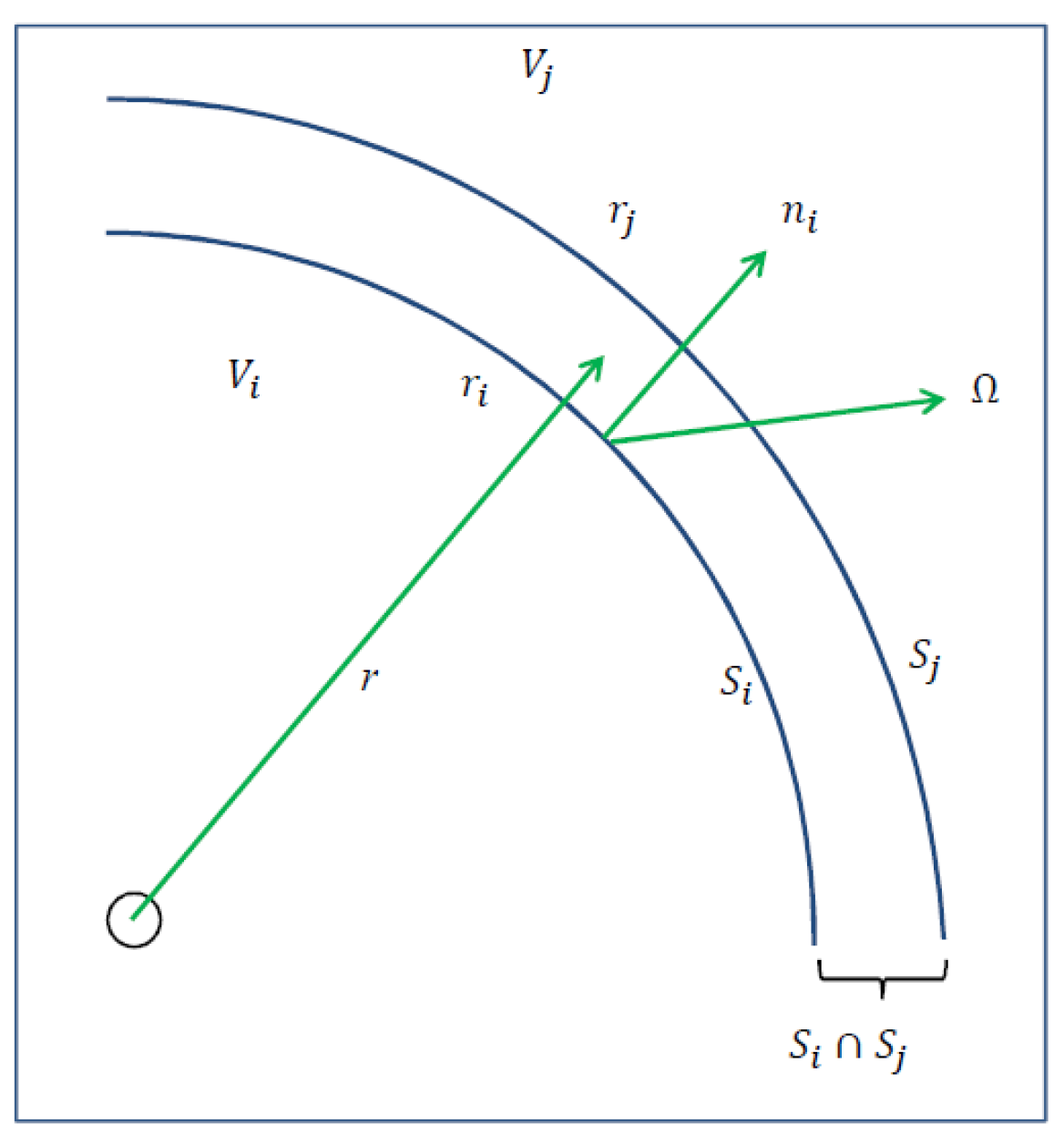
However, as regards that the purpose is to achieve a principle that admits discontinuous TF, hence another error should be added too. The nature of this error is based on failing to satisfy the interface continuity condition between two elements having volumes $V_i$ and $V_j$. According to Figure 1, when two elements are considered separated and it is assumed that there is no connection between them, then the error ${\epsilon }_f$ is appeared. Hence, an overall error measure $e{r}_{\lambda }$ is obtained by adding the three error measures and is given by:

$$e{r}_{\lambda }\left(\phi \right)={\epsilon }_V+{\epsilon }_{\partial V}+{\epsilon }_f,$$

(19)

with definitions:

$$\begin{array}{cc}{\epsilon }_V\left({\phi }^{+}\right)={{\displaystyle \int }}_V{{\displaystyle \int }}_{4\pi }& \left[\left\{\overrightarrow{\mathsf{\Omega }}.\overrightarrow{\nabla }{\phi }^{+}+G^{-1}{\phi }^{-}{}_0-Q^{-}\right\}G\left\{\overrightarrow{\mathsf{\Omega }}.\overrightarrow{\nabla }{\phi }^{+}+G^{-1}{\phi }^{-}{}_0-Q^{-}\right\}\right]\\ & \hfill +\left[\left\{\overrightarrow{\mathsf{\Omega }}.\overrightarrow{\nabla }{\phi }^{-}{}_0+\mathrm{C}{\phi }^{+}-Q^{+}\right\}{C}^{-1}\left\{\overrightarrow{\mathsf{\Omega }}.\overrightarrow{\nabla }{\phi }^{-}{}_0+\mathrm{C}{\phi }^{+}-Q^{+}\right\}\right]d\mathsf{\Omega }dV\end{array}$$

(20)

$${\epsilon }_{\partial V}\left({\phi }^{+}\right)=2{{\displaystyle \int }}_{\partial V}{{\displaystyle \int }}_{\overrightarrow{\mathsf{\Omega }}.\overrightarrow{n}<0}\left|\overrightarrow{\mathsf{\Omega }}.\overrightarrow{n}\right|\left[{\phi }^{+}\left(\overrightarrow{r},\overrightarrow{\mathsf{\Omega }}\right)-{\phi }^{+}{}_0\left(\overrightarrow{r},\overrightarrow{\mathsf{\Omega }}\right)\right]d\mathsf{\Omega }dS,$$

(21)

and

$${\epsilon }_f=\lambda {{\displaystyle \int }}_{\cup (S_i\cap S_j)}{{\displaystyle \int }}_{4\pi }\left\{\overrightarrow{\mathsf{\Omega }}.{\overrightarrow{n}}_i\left[\phi \left(\overrightarrow{r_i},\overrightarrow{\mathsf{\Omega }}\right)-\phi \left(\overrightarrow{r_j},\overrightarrow{\mathsf{\Omega }}\right)\right]\times {\Sigma }^{-1}\overrightarrow{\mathsf{\Omega }}.{\overrightarrow{n}}_i\left[\phi \left(\overrightarrow{r_i},\overrightarrow{\mathsf{\Omega }}\right)-\phi \left(\overrightarrow{r_j},\overrightarrow{\mathsf{\Omega }}\right)\right]\right\}d\mathsf{\Omega }dS,$$

(22)

where, with employing the even and odd parts of AF, the ${\epsilon }_f$ error reduced to:

$$\lambda {{\displaystyle \int }}_{\cup \left(S_i\cap S_j\right)}{{\displaystyle \int }}_{4\pi }\left(\begin{array}{c}\left\{\overrightarrow{\mathsf{\Omega }}.{\overrightarrow{n}}_i\left[{\phi }^{+}\left(\overrightarrow{r_i},\overrightarrow{\mathsf{\Omega }}\right)-{\phi }^{+}\left(\overrightarrow{r_j},\overrightarrow{\mathsf{\Omega }}\right)\right]\right\}G\\ \times \left\{\overrightarrow{\mathsf{\Omega }}.{\overrightarrow{n}}_i\left[{\phi }^{+}\left(\overrightarrow{r_i},\overrightarrow{\mathsf{\Omega }}\right)-{\phi }^{+}\left(\overrightarrow{r_j},\overrightarrow{\mathsf{\Omega }}\right)\right]\right\}\\ +\left\{\overrightarrow{\mathsf{\Omega }}.{\overrightarrow{n}}_i\left[{\phi }^{-}\left(\overrightarrow{r_i},\overrightarrow{\mathsf{\Omega }}\right)-{\phi }^{-}\left(\overrightarrow{r_j},\overrightarrow{\mathsf{\Omega }}\right)\right]\right\}{C}^{-1}\\ \times \left\{\overrightarrow{\mathsf{\Omega }}.{\overrightarrow{n}}_i\left[{\phi }^{-}\left(\overrightarrow{r_i},\overrightarrow{\mathsf{\Omega }}\right)-{\phi }^{-}\left(\overrightarrow{r_j},\overrightarrow{\mathsf{\Omega }}\right)\right]\right\}\end{array}\right)d\mathsf{\Omega }dS.$$

(23)

Now, by collecting the introduced errors, the functional $V_{\lambda }\left(\phi \right)$, which is a generalized least-squares measure of the amounts by which the trial function $\phi$ fails to satisfy the first-order Boltzmann equation and the interface and boundary condition, can be obtained.

$$\begin{array}{ll}e{r}_{\lambda }\left({\phi }^{+},{\phi }^{-}\right)& \\ ={{\displaystyle \int }}_V\left\{\begin{array}{c}<\overrightarrow{\mathsf{\Omega }}.\overrightarrow{\nabla }{\phi }^{-}{}_0+C{\phi }^{+}-Q^{+},C^{-1}\\ \times \left[\overrightarrow{\mathsf{\Omega }}.\overrightarrow{\nabla }{\phi }^{-}{}_0+C{\phi }^{+}-Q^{+}\right]>\\ +<\overrightarrow{\mathsf{\Omega }}.\overrightarrow{\nabla }{\phi }^{+}+G^{-1}{\phi }^{-}{}_0-Q^{-},G\\ \times \left[\overrightarrow{\mathsf{\Omega }}.\overrightarrow{\nabla }{\phi }^{+}+G^{-1}{\phi }^{-}{}_0-Q^{-}\right]>\end{array}\right\}dV& \\ +2{{\displaystyle \int }}_{\partial V}{{\displaystyle \int }}_{\overrightarrow{\mathsf{\Omega }}.\overrightarrow{n}<0}\left|\overrightarrow{\mathsf{\Omega }}.\overrightarrow{n}\right|{\left[T-{\phi }^{+}-{\phi }^{-}{}_0\right]}^{2}d\mathsf{\Omega }dS& \\ +\lambda {{\displaystyle \int }}_{\cup \left(S_i\cap S_j\right)}{{\displaystyle \int }}_{4\pi }\left(\begin{array}{c}\left\{\overrightarrow{\mathsf{\Omega }}.{\overrightarrow{n}}_i\left[{\phi }^{+}\left(\overrightarrow{r_i},\overrightarrow{\mathsf{\Omega }}\right)-{\phi }^{+}\left(\overrightarrow{r_j},\overrightarrow{\mathsf{\Omega }}\right)\right]\right\}G\\ \times \left\{\overrightarrow{\mathsf{\Omega }}.{\overrightarrow{n}}_i\left[{\phi }^{+}\left(\overrightarrow{r_i},\overrightarrow{\mathsf{\Omega }}\right)-{\phi }^{+}\left(\overrightarrow{r_j},\overrightarrow{\mathsf{\Omega }}\right)\right]\right\}\\ +\left\{\overrightarrow{\mathsf{\Omega }}.{\overrightarrow{n}}_i\left[{\phi }^{-}\left(\overrightarrow{r_i},\overrightarrow{\mathsf{\Omega }}\right)-{\phi }^{-}\left(\overrightarrow{r_j},\overrightarrow{\mathsf{\Omega }}\right)\right]\right\}{C}^{-1}\\ \times \left\{\overrightarrow{\mathsf{\Omega }}.{\overrightarrow{n}}_i\left[{\phi }^{-}\left(\overrightarrow{r_i},\overrightarrow{\mathsf{\Omega }}\right)-{\phi }^{-}\left(\overrightarrow{r_j},\overrightarrow{\mathsf{\Omega }}\right)\right]\right\}\end{array}\right)d\mathsf{\Omega }dS.& \end{array}$$

(24)

Using the generalized least-square method and with respect to the special properties of the operator’s leakage $G$ and removal $C$ (self-adjoint and definite positive) and the divergence theorem, the important maximum principle can be derived as

$$\begin{array}{ll}{K}_{\lambda }^{+}\left[{\phi }^{+}\right]={{\displaystyle \int }}_V{{\displaystyle \int }}_{4\pi }& \left\{\overrightarrow{\mathsf{\Omega }}.\overrightarrow{\nabla }{\phi }_1^{+}G\left[\overrightarrow{\mathsf{\Omega }}.\overrightarrow{\nabla }{\phi }_2^{+}\right]+{\phi }_1^{+}C{\phi }_2^{+}\right\}d\mathsf{\Omega }dV+{{\displaystyle \int }}_{\partial V}{{\displaystyle \int }}_{4\pi }\left|\overrightarrow{\mathsf{\Omega }}.\overrightarrow{n}\right|{\phi }_1^{+}{\phi }_2^{+}d\mathsf{\Omega }dS\\ & \begin{array}{ll}+{{\displaystyle \int }}_V{{\displaystyle \int }}_{4\pi }\left\{{\phi }_1^{+}{Q}^{+}+\overrightarrow{\mathsf{\Omega }}.\overrightarrow{\nabla }{\phi }_1^{+}G{Q}^{-}\right\}d\mathsf{\Omega }dV& \\ +{{\displaystyle \int }}_{Ss}{{\displaystyle \int }}_{\overrightarrow{\mathsf{\Omega }}.\overrightarrow{n}<0}\left|\overrightarrow{\mathsf{\Omega }}.\overrightarrow{n}\right|\left\{{\phi }_1^{+}\left(\overrightarrow{r},\overrightarrow{\mathsf{\Omega }}\right)+{\phi }_1^{+}\left(\overrightarrow{r},-\overrightarrow{\mathsf{\Omega }}\right)\right\}T\left(\overrightarrow{r},\overrightarrow{\mathsf{\Omega }}\right)d\mathsf{\Omega }dS& \\ -\lambda {{\displaystyle \int }}_{\cup (S_i\cap S_j)}{{\displaystyle \int }}_{4\pi }\left\{\overrightarrow{\mathsf{\Omega }}.{\overrightarrow{n}}_i\left[{\phi }^{+}\left(\overrightarrow{r_i},\overrightarrow{\mathsf{\Omega }}\right)-{\phi }^{+}\left(\overrightarrow{r_j},\overrightarrow{\mathsf{\Omega }}\right)\right]\right\}& \\ \times G\left\{\overrightarrow{\mathsf{\Omega }}.{\overrightarrow{n}}_i\left[{\phi }^{+}\left(\overrightarrow{r_i},\overrightarrow{\mathsf{\Omega }}\right)-{\phi }^{+}\left(\overrightarrow{r_j},\overrightarrow{\mathsf{\Omega }}\right)\right]\right\}d\mathsf{\Omega }dS.& \end{array}\end{array}$$

(25)

In addition, the formulation of classical principle has been derived in [18], which is based on only the volume component of error and the boundary error functional and again using the generalized least-square method and algebraic operators, the maximum principles that admit the continuous TFs in space and angular variables, can be written as:

$$K^{+}\left[{\phi }^{+}\right]=2F_s^{+}\left[{\phi }^{+}\right]-F_s^{+}\left[{\phi }^{+},{\phi }^{+}\right],$$

(26)

where

$$F_s^{+}\left[{\phi }_1^{+},{\phi }_2^{+}\right]={{\displaystyle \int }}_V{{\displaystyle \int }}_{4\pi }\left\{\overrightarrow{\mathsf{\Omega }}.\overrightarrow{\nabla }{\phi }_1^{+}G\left[\overrightarrow{\mathsf{\Omega }}.\overrightarrow{\nabla }{\phi }_2^{+}\right]+{\phi }_1^{+}C{\phi }_2^{+}\right\}d\mathsf{\Omega }dV+{{\displaystyle \int }}_{\partial V}{{\displaystyle \int }}_{4\pi }\left|\overrightarrow{\mathsf{\Omega }}.\overrightarrow{n}\right|{\phi }_1^{+}{\phi }_2^{+}d\mathsf{\Omega }dS,$$

(27)

and

$$\begin{array}{ll}{F}_s^{+}\left[{\phi }_1^{+}\right]={{\displaystyle \int }}_V{{\displaystyle \int }}_{4\pi }& \left\{{\phi }_1^{+}{Q}^{+}+\overrightarrow{\mathsf{\Omega }}.\overrightarrow{\nabla }{\phi }_1^{+}G{Q}^{-}\right\}d\mathsf{\Omega }dV\\ & +{{\displaystyle \int }}_{S_i}{{\displaystyle \int }}_{\overrightarrow{\mathsf{\Omega }}.\overrightarrow{n}<0}\left|\overrightarrow{\mathsf{\Omega }}.\overrightarrow{n}\right|\left\{{\phi }_1^{+}\left(\overrightarrow{r},\overrightarrow{\mathsf{\Omega }}\right)+{\phi }_1^{+}\left(\overrightarrow{r},-\overrightarrow{\mathsf{\Omega }}\right)\right\}T\left(\overrightarrow{r},\overrightarrow{\mathsf{\Omega }}\right)d\mathsf{\Omega }dS,\end{array}$$

(28)

and the complementary of this principle is:

$$K^{-}\left[{\phi }^{-}\right]=2F_s^{-}\left[{\phi }^{-}\right]-F_s^{-}\left[{\phi }^{-},{\phi }^{-}\right],$$

(29)

where

$$\begin{array}{ll}{F}_s^{-}\left[{\phi }_1^{-},{\phi }_2^{-}\right]=& {{\displaystyle \int }}_V{{\displaystyle \int }}_{4\pi }\left\{\overrightarrow{\mathsf{\Omega }}.\overrightarrow{\nabla }{\phi }_1^{-}{C}^{-1}\left[\overrightarrow{\mathsf{\Omega }}.\overrightarrow{\nabla }{\phi }_2^{-}\right]+{\phi }_1^{-}{G}^{-1}{\phi }_2^{-}\right\}d\mathsf{\Omega }dV\\ & +{{\displaystyle \int }}_{S_b\cup S_s}{{\displaystyle \int }}_{4\pi }\left|\overrightarrow{\mathsf{\Omega }}.\overrightarrow{n}\right|{\phi }_1^{-}{\phi }_2^{-}d\mathsf{\Omega }dS,\end{array}$$

(30)

and

$$\begin{array}{ll}{F}_s^{-}\left[{\phi }_1^{-}\right]={{\displaystyle \int }}_V{{\displaystyle \int }}_{4\pi }& \left\{{\phi }_1^{-}{S}^{-}+\overrightarrow{\mathsf{\Omega }}.\overrightarrow{\nabla }{\phi }_1^{-}{C}^{-1}{S}^{+}\right\}d\mathsf{\Omega }dV\\ & +{{\displaystyle \int }}_{S_i}{{\displaystyle \int }}_{\overrightarrow{\mathsf{\Omega }}.\overrightarrow{n}<0}\left|\overrightarrow{\mathsf{\Omega }}.\overrightarrow{n}\right|\left\{{\phi }_1^{-}\left(\overrightarrow{r},\overrightarrow{\mathsf{\Omega }}\right)+{\phi }_1^{-}\left(\overrightarrow{r},-\overrightarrow{\mathsf{\Omega }}\right)\right\}T\left(\overrightarrow{r},\overrightarrow{\mathsf{\Omega }}\right)d\mathsf{\Omega }dS,\end{array}$$

(31)

Now, through comprehensive observation of Equation (25) and making a comparison between the first three terms of Equations (27) and (28), the maximum principle $K_{\lambda }^{+}\left[{\phi }^{+}\right]$ can be reduced to

$$\begin{array}{ll}{K}_{\lambda }^{+}\left[{\phi }^{+}\right]=K^{+}\left[{\phi }^{+}\right]& \\ & -\lambda {{\displaystyle \int }}_{\cup (S_i\cap S_j)}{{\displaystyle \int }}_{4\pi }\left\{\mathsf{\Omega }.n_i\left[{\phi }^{+}\left(\overrightarrow{r_i},\overrightarrow{\mathsf{\Omega }}\right)-{\phi }^{+}\left(\overrightarrow{r_j},\overrightarrow{\mathsf{\Omega }}\right)\right]\right\}\\ & \times G\left\{\mathsf{\Omega }.n_i\left[{\phi }^{+}\left(\overrightarrow{r_i},\overrightarrow{\mathsf{\Omega }}\right)-{\phi }^{+}\left(\overrightarrow{r_j},\overrightarrow{\mathsf{\Omega }}\right)\right]\right\}d\mathsf{\Omega }dS.\end{array}$$

(32)

Here, $\left[{\phi }^{+}\left(\overrightarrow{r_i},\overrightarrow{\mathsf{\Omega }}\right)-{\phi }^{+}\left(\overrightarrow{r_j},\overrightarrow{\mathsf{\Omega }}\right)\right]$ is the jump in the TF at $\overrightarrow{r}$ on the interface $(S_i\cap S_j)$, and $\lambda$ is a positive number called penalty parameter and it has the role of controlling the jump in the approximate solution at interfaces.

3.1. The Directional Dependence of the AF

The spherical harmonics, or $P_N$, is one of the most popular methods for describing the directional dependence of AF, which is used in this study. They can produce a high-quality approximation for the angular dependence even when a relatively small number of basis functions are employed, particularly when the solution is closed to isotropic. Thus, the $P_N$ method can be used to accurately model a wide variety of neutron transport problems.

In one dimensional geometry, the angular dependence of the EAOP flux is expressed in terms of even and odd order Legendre polynomials, respectively. Thus, the EAOP flux can be approximated by the TFs with definitions:

$${\phi }^{+}\left(x,\mu \right)={\displaystyle \sum }_{l\left(even\right)}^N\left(\frac{2l+1}{2}\right)P_l\left(\mu \right){\phi }_l^{+}\left(x\right),$$

(33)

and

$${\phi }^{-}\left(x,\mu \right)={\displaystyle \sum }_{l\left(odd\right)}^N\left(\frac{2l+1}{2}\right)P_l\left(\mu \right){\phi }_l^{-}\left(x\right),$$

(34)

also, the even parity TF for two dimensional can be written as

$${\phi }^{+}\left(x,y,\mu ,\omega \right)={\displaystyle \sum }_{l\left(even\right)}^N{\displaystyle \sum }_{m\left(even\right)}^l\left[Y_{lm}^o\left(\mu ,\omega \right){\phi }_{lm}^{+o}\left(x,y\right)+Y_{lm}^e\left(\mu ,\omega \right){\phi }_{lm}^{+e}\left(x,y\right)\right],$$

(35)

where

$$\left(\begin{array}{c}{Y}_{lm}^o\left(\mu ,\omega \right)\\ Y_{lm}^e\left(\mu ,\omega \right)\end{array}\right)=\sqrt{\left[\frac{\left(2l+1\right)}{4\pi }\left(2-{\delta }_{l,0}\right)\frac{\left(l-m\right)}{\left(l+m\right)}\right]}{P}_l^m\left(\mu \right)\left(\begin{array}{c}sin\left(m\omega \right)\\ cos\left(m\omega \right)\end{array}\right).$$

(36)

The series expansions of the AF into angular basis functions can be written in matrix notation as:

$${\phi }^{+}\left(\overrightarrow{r},\overrightarrow{\mathsf{\Omega }}\right)=W^{+T}\left(\overrightarrow{\mathsf{\Omega }}\right){\phi }^{+}\left(\overrightarrow{r}\right),$$

(37)

and

$${\phi }^{-}\left(\overrightarrow{r},\overrightarrow{\mathsf{\Omega }}\right)=W^{-T}\left(\overrightarrow{\mathsf{\Omega }}\right){\phi }^{-}\left(\overrightarrow{r}\right).$$

(38)

where the transposed vectors $W^{+T}$ and $W^{-T}$ represent the EAOP angular basis functions, respectively, for corresponding one- and two-dimensional geometries.

3.2. Finite Element TFs for Spatial Domain

There are some approaches for verifying spatial discretization of the $P_N$ TE. However, in this paper, the spatial dependence of the even-parity AF is presented in terms of the nodal values of the flux and the FE shape functions. For this purpose, the even parity flux for each element can thus be approximated by the trial functions ${\phi }^{+}\left(r,\mathsf{\Omega }\right)$ as

$${\phi }^{+}\left(\overrightarrow{r},\overrightarrow{\mathsf{\Omega }}\right)={\displaystyle \sum }_{e=1}^E{\phi }^{+e}\left(\overrightarrow{r},\overrightarrow{\mathsf{\Omega }}\right)={\displaystyle \sum }_{e=1}^E{\displaystyle \sum }_{l\left(even\right)}^{N-1}{\displaystyle \sum }_{i=1}^{N_e}{B}_i^e\left(\overrightarrow{r}\right)W_l^{+}(\overrightarrow{\mathsf{\Omega }}){\phi }_{il}^{+e},$$

(39)

where $N_e$ is the number of nodes in each element, which can vary from region to region. The Equation (39) can be written in compact notations as:

$${\phi }^{+}\left(\overrightarrow{r},\overrightarrow{\mathsf{\Omega }}\right)={\displaystyle \sum }_{e=1}^E{B}^{eT}\left(\overrightarrow{r}\right)\otimes W^{+T}\left(\overrightarrow{\mathsf{\Omega }}\right){\phi }^{+e},$$

(40)

and with a similar procedure, the odd parity flux appears as

$${\phi }^{-}\left(\overrightarrow{r},\overrightarrow{\mathsf{\Omega }}\right)={\displaystyle \sum }_{e=1}^E{\phi }^{-e}\left(\overrightarrow{r},\overrightarrow{\mathsf{\Omega }}\right)={\displaystyle \sum }_{e=1}^E{\displaystyle \sum }_{l\left(odd\right)}^{N+1}{\displaystyle \sum }_{i=1}^{N_e}{B}_i^e\left(\overrightarrow{r}\right)W_l^{-}(\overrightarrow{\mathsf{\Omega }}){\phi }_{il}^{-e}.$$

(41)

Again, the matrix form of this expression is given by

$${\phi }^{-}\left(\overrightarrow{r},\overrightarrow{\mathsf{\Omega }}\right)={\displaystyle \sum }_{e=1}^E{B}^{eT}\left(\overrightarrow{r}\right)\otimes W^{-T}\left(\overrightarrow{\mathsf{\Omega }}\right){\phi }^{-e}.$$

(42)

3.3. The Maximization of the VP

The maximum principles, given by $K^{+}\left[{\phi }^{+}\right]$ and $K^{-}\left[{\phi }^{-}\right]$ functionals, which admit continuous TFs, have been derived in [26]. The TFs used in these principles are forced to obey the continuity conditions at the interfaces between elements. However, in the DFE approach, there is another situation. The maximum principle, given by $K_{\lambda }^{+}\left[{\phi }^{+}\right]$ functional, admits both continuous TFs and discontinuous TFs. Unlike the continuous case, the discontinuous TFs do not have to obey the continuity conditions at interfaces between elements. Hence, generally, there are two different approaches for implementation of the FEM on the TF. According to the first approach, all the elements are completely connected with the adjacent elements. It means that the continuity condition between the adjacent elements is established. Hence, this approach is used for the classical principle, which admits continuous TF. However, the main objective of this paper is based on analyzing the various discontinuous aspects of the FEM.

In the discontinuous approach, two types of discontinuities can be considered between adjacent regions or adjacent elements of each region, which are called region-wise technique and element-wise technique, respectively. In the first case, a continuous flux profile is assumed to exist within the interior of the regions of the system, while discontinuities are allowed at the interfaces between these regions. In the second case, a totally discontinuous mesh is considered where the TFs are allowed to be discontinuous at all interfaces between adjacent elements. These two approaches for two-dimensional geometries are shown schematically in Figure 2.

In global terms, the reduced functional of $K_{\lambda }^{+}\left[{\phi }^{+}\right]$ can be written as

$$K_{\lambda }^{+}\left[{\phi }^{+}\right]=K^{+}\left[{\phi }^{+}\right]-{\displaystyle \sum }_{i=1}^{N_f}{I}_i\left[{\phi }^{+}\left(\overrightarrow{r_i},\overrightarrow{\mathsf{\Omega }}\right)\right],$$

(43)

where the interfacial functional $I_i$ is expressed as

$$\begin{array}{ll}{I}_i\left[{\phi }^{+}\right]={\lambda }_i{{\displaystyle \int }}_{\cup \left(S_i\cap S_j\right)}& \left\{\overrightarrow{\mathsf{\Omega }}.{\overrightarrow{n}}_i\left[{\phi }^{+}\left(\overrightarrow{r_i},\overrightarrow{\mathsf{\Omega }}\right)-{\phi }^{+}\left(\overrightarrow{r_j},\overrightarrow{\mathsf{\Omega }}\right)\right]\right\}\\ & \hspace{1em}\hspace{1em}\times G\left\{\overrightarrow{\mathsf{\Omega }}.{\overrightarrow{n}}_i\left[{\phi }^{+}\left(\overrightarrow{r_i},\overrightarrow{\mathsf{\Omega }}\right)-{\phi }^{+}\left(\overrightarrow{r_j},\overrightarrow{\mathsf{\Omega }}\right)\right]\right\}d\mathsf{\Omega }dS.\end{array}$$

(44)

In addition, $N_f$ is the number of interfaces around each element, which is illustrated for various types of elements in Figure 3.

By inserting the even parity TF into Equation (43), the local stiffness matrix $A^{+}$ for each element and an interface matrix $A_f^{+}$ for each interface can be obtained. After performing the assembling procedure, the following discretized functional holds:

$$K_{\lambda }^{+}\left[{\phi }^{+}\right]=2{\phi }^{+T}{B}^{+}-{\phi }^{+T}{A}^{+}{\phi }^{+}-{\phi }^{+T}{A}_f^{+}{\phi }^{+},$$

(45)

where the local stiffness matrix $A^{+}$, obtained in this case, is the same as was obtained in $K^{+}$ principle.

Requiring $K_{\lambda }^{+}\left[{\phi }^{+}\right]$ to be stationary with respect to variations of each component of $\left[{\phi }^{+}\right]$ yields:

$$\frac{\partial K_{\lambda }^{+}}{\partial {\phi }^{+T}}=0\Rightarrow \left(A^{+}+A_f^{+}\right){\phi }^{+}=B^{+},$$

(46)

where the GM $\left(A^{+}+A_f^{+}\right)$ is symmetric, positive-definite, and because of the local compact support, also sparse and banded.

The essential difference from the calculations viewpoint between $K^{+}$ principle and $K_{\lambda }^{+}$ principle is to form the GM. In the continuous case, all the local matrixes are assembled as ordinary, which was introduced in Cassiano et al. [27]. However, in the principle, which is based on the DFE, the stiffness matrixes of interfacial elements are located next to each other without any assembling, and then, the interfacial matrix couple local matrixes. According to this, different orders of angular approximations can be considered in various regions.

3.4. Influence of the Penalty Parameter

A simple treatment is given here for the influence of the penalty parameter $\lambda$ on a discontinuous variational approximation for the AF, which is given by the discontinuous variational approximations for the even and odd parity AFs. In fact, the penalty parameter is used to control the discontinuity range of elements. As a result of this, when the penalty parameter is increased, the jump at the interfaces is reduced. This remark suggests that there may be some specific values of $\lambda$ for which a DFE solution is superior to a classical continuous variational solution [17].

For specifying the penalty parameter in applying $K_{\lambda }^{+}\left[{\phi }^{+}\right]$, some appropriate cases are recommended. Generally, by using a high value (physical infinite) for $\lambda$, the solutions tend to continuous solutions. However, in multi-region problems, the value of $\lambda$ is defined with respect to the properties of each region, and hence $\lambda =\frac{1}{h}$, where h is element width, can be considered as a choice for the penalty parameter. Another possible choice for the penalty parameter is $=0$.

3.5. DFE with the Element by Element NC

The maximum principle based on the DFE can be imposed with only a single discontinuous trial function (TF). However, in the sequel a general maximum principle $K_{\lambda }^c\left({\phi }^{+},{\phi }^{-},{\theta }^{+},{\theta }^{-}\right)$ can be considered with the penalty parameter non-negative, so that the degree of control on discontinuities is varied from none for $\lambda =0$ to their extinction as $\lambda \to \infty$. In this approach of DFE, two TFs are used. The TFs ${\phi }^{+}$ and ${\phi }^{-}$ are continuous across interfaces, and they couple the elements into each other. In addition, ${\theta }^{+}$ and ${\theta }^{-}$ are the helping TFs to ensure element by element NC and, within an element, are functions of neutron direction only. In this section, the new maximum principle based on DFE and element by element NC is derived.

Specification of TFs

Over the whole system, the expression used for classical components ${\psi }^{\pm }\left(\overrightarrow{r},\overrightarrow{\mathsf{\Omega }}\right)$ of the discontinuous TFs ${\phi }^{\pm }\left(\overrightarrow{r},\overrightarrow{\mathsf{\Omega }}\right)$ are of the kind

$${\psi }^{\pm }\left(\overrightarrow{r},\overrightarrow{\mathsf{\Omega }}\right)={\displaystyle \sum }_{m=1}^M{\displaystyle \sum }_{l=1}^{L^{\pm }}{a}^{\pm }{}_{ml}{\psi }^{\pm }{}_{ml}\left(\overrightarrow{r},\overrightarrow{\mathsf{\Omega }}\right)\hspace{1em}\hspace{1em}m=1,2,\dots M$$

(47)

for an FE spatial mesh with M nodes. In the following, a general representation for the discontinuous components ${\theta }^{\pm }$ of the TF ${\phi }^{\pm }\left(r,\mathsf{\Omega }\right)$ can be written as

$${\theta }^{\pm }\left(\overrightarrow{r},\overrightarrow{\mathsf{\Omega }}\right)={\displaystyle \sum }_{i=1}^I{\displaystyle \sum }_{l=1}^{L^{\pm }}{b}^{\pm }{}_{ml}{\theta }^{\pm }{}_{il}\left(\overrightarrow{r},\overrightarrow{\mathsf{\Omega }}\right),$$

(48)

where outside of element $i$ the basis functions ${\theta }^{\pm }{}_{il}\left(\overrightarrow{r},\overrightarrow{\mathsf{\Omega }}\right)$ vanish.

3.6. New Formulated of ${\mathrm{K}}_{\mathsf{\lambda }}\left[\mathsf{\phi }\right]$

The $K_{\lambda }\left[\phi \right]$ maximum principle for the first order Boltzmann equation, which is given by [16] can be expressed as

$$\begin{array}{ll}{K}_{\lambda }\left(\phi \right)=& \underset{V}{{\displaystyle \int }}[2\langle \phi ,Q\rangle +2\langle \overrightarrow{\mathsf{\Omega }}.\overrightarrow{\nabla }\phi ,{\Sigma }^{-1}Q\rangle ]dV-\tilde{F}\left(\phi ,\phi \right)\\ & \hspace{1em}\hspace{1em}\hspace{1em}\begin{array}{ll}+4{{\displaystyle \int }}_V{{\displaystyle \int }}_{\overrightarrow{\mathsf{\Omega }}.\overrightarrow{n}<0}\left|\overrightarrow{\mathsf{\Omega }}.\overrightarrow{n}\right|\phi Td\mathsf{\Omega }dS-{{\displaystyle \int }}_{\cup S_i}{{\displaystyle \int }}_{4\pi }{\phi }^2\overrightarrow{\mathsf{\Omega }}.{\overrightarrow{n}}_{i}d\mathsf{\Omega }dS& \\ -\lambda {{\displaystyle \int }}_{\cup \left(s_i\cap s_j\right)}{{\displaystyle \int }}_{4\pi }\{\overrightarrow{\mathsf{\Omega }}.{\overrightarrow{n}}_i[\phi (\overrightarrow{r_i},\overrightarrow{\mathsf{\Omega }})-\phi (\overrightarrow{r_j},\overrightarrow{\mathsf{\Omega }})]\}{\Sigma }^{-1}& \\ \times {{\displaystyle \int }}_{4\pi }\{\overrightarrow{\mathsf{\Omega }}.{\overrightarrow{n}}_i[\phi (\overrightarrow{r_i},\overrightarrow{\mathsf{\Omega }})-\phi (\overrightarrow{r_j},\overrightarrow{\mathsf{\Omega }})]\}d\mathsf{\Omega }dS,& \end{array}\end{array}$$

(49)

where the bilinear functional $\tilde{F}\left(\phi ,\phi \right)$ for arbitrary $p(\overrightarrow{r},\overrightarrow{\mathsf{\Omega }})$ and $v(\overrightarrow{r},\overrightarrow{\mathsf{\Omega }})$ is defined as:

$$\tilde{F}\left(p,v\right)={{\displaystyle \int }}_V[\langle \overrightarrow{\mathsf{\Omega }}.\overrightarrow{\nabla }p,{\Sigma }^{-1}\overrightarrow{\mathsf{\Omega }}.\overrightarrow{\nabla }v\rangle +\langle p,\Sigma v\rangle ]dV+{{\displaystyle \int }}_{\partial V}{{\displaystyle \int }}_{4\pi }\left|\overrightarrow{\mathsf{\Omega }}.\overrightarrow{n}\right|pvd\mathsf{\Omega }dS.$$

(50)

Equation (48) is derived from the identity

$$K_{\lambda }\left(\phi \right)+e{r}_{\lambda }\left(\phi \right)=2\alpha ,$$

(51)

where the definition of the error functional is

$$\begin{array}{ll}e{r}_{\lambda }\left(\phi \right)=& {{\displaystyle \int }}_V\langle \overrightarrow{\mathsf{\Omega }}.\overrightarrow{\nabla }\phi ,\Sigma \phi -Q,{\Sigma }^{-1}(\overrightarrow{\mathsf{\Omega }}.\overrightarrow{\nabla }\phi +\Sigma \phi -Q)\rangle dV\\ & \hspace{1em}\hspace{1em}\hspace{1em}\hspace{1em}+2{{\displaystyle \int }}_{\partial V}{{\displaystyle \int }}_{\overrightarrow{\mathsf{\Omega }}.\overrightarrow{n}<0}\left|\overrightarrow{\mathsf{\Omega }}.\overrightarrow{n}\right|{\left[T-\phi \right]}^{2}d\mathsf{\Omega }dS\\ & \hspace{1em}\hspace{1em}\hspace{1em}\hspace{1em}+\lambda {{\displaystyle \int }}_{\cup \left(S_i\cap S\right)}{{\displaystyle \int }}_{4\pi }\{\overrightarrow{\mathsf{\Omega }}.{\overrightarrow{n}}_i[\phi ({\overrightarrow{r}}_i,\overrightarrow{\mathsf{\Omega }})-\phi ({\overrightarrow{r}}_j,\overrightarrow{\mathsf{\Omega }})]\}{\Sigma }^{-1}\\ & \hspace{1em}\hspace{1em}\hspace{1em}\hspace{1em}\times \{\overrightarrow{\mathsf{\Omega }}.{\overrightarrow{n}}_i[\phi ({\overrightarrow{r}}_i,\overrightarrow{\mathsf{\Omega }})-\phi ({\overrightarrow{r}}_j,\overrightarrow{\mathsf{\Omega }})]\}d\mathsf{\Omega }dS,\end{array}$$

(52)

and

$$2\alpha =\underset{V}{{\displaystyle \int }}\langle Q,{\Sigma }^{-1}Q\rangle dV+2{{\displaystyle \int }}_{\partial V}{{\displaystyle \int }}_{\overrightarrow{\mathsf{\Omega }}.\overrightarrow{n}}\left|\overrightarrow{\mathsf{\Omega }}.\overrightarrow{n}\right|T^{2}d\mathsf{\Omega }dS.$$

(53)

The functional $e{r}_{\lambda }\left(\phi \right)$ can be written, based on parity components of AF, as

$$\begin{array}{ll}e{r}_{\lambda }\left({\phi }^{+},{\phi }^{-}\right)=& {{\displaystyle \int }}_V\left\{\begin{array}{c}<\overrightarrow{\mathsf{\Omega }}.\overrightarrow{\nabla }{\phi }^{-}+C{\phi }^{+}-Q^{+},C^{-1}\\ \times \left[\overrightarrow{\mathsf{\Omega }}.\overrightarrow{\nabla }{\phi }^{-}+C{\phi }^{+}-Q^{+}\right]>\\ +<\overrightarrow{\mathsf{\Omega }}.\overrightarrow{\nabla }{\phi }^{+}+G^{-1}{\phi }^{-}-Q^{-},G\\ \times \left[\overrightarrow{\mathsf{\Omega }}.\overrightarrow{\nabla }{\phi }^{+}+G^{-1}{\phi }^{-}-Q^{-}\right]>\end{array}\right\}dV\\ & \hspace{1em}+2{{\displaystyle \int }}_{\partial V}{{\displaystyle \int }}_{\overrightarrow{\mathsf{\Omega }}.\overrightarrow{n}<0}\left|\overrightarrow{\mathsf{\Omega }}.\overrightarrow{n}\right|{\left[T-{\phi }^{+}-{\phi }^{-}\right]}^{2}d\mathsf{\Omega }dS\\ & \hspace{1em}+\lambda {{\displaystyle \int }}_{\cup \left(S_i\cap S_j\right)}{{\displaystyle \int }}_{4\pi }\left(\begin{array}{c}\left\{\overrightarrow{\mathsf{\Omega }}.{\overrightarrow{n}}_i\left[{\phi }^{+}\left({\overrightarrow{r}}_i,\overrightarrow{\mathsf{\Omega }}\right)-{\phi }^{+}\left({\overrightarrow{r}}_j,\overrightarrow{\mathsf{\Omega }}\right)\right]\right\}G\\ \times \left\{\overrightarrow{\mathsf{\Omega }}.{\overrightarrow{n}}_i\left[{\phi }^{+}\left({\overrightarrow{r}}_i,\overrightarrow{\mathsf{\Omega }}\right)-{\phi }^{+}\left({\overrightarrow{r}}_j,\overrightarrow{\mathsf{\Omega }}\right)\right]\right\}\\ +\left\{\overrightarrow{\mathsf{\Omega }}.{\overrightarrow{n}}_i\left[{\phi }^{-}\left({\overrightarrow{r}}_i,\overrightarrow{\mathsf{\Omega }}\right)-{\phi }^{-}\left({\overrightarrow{r}}_j,\overrightarrow{\mathsf{\Omega }}\right)\right]\right\}{C}^{-1}\\ \times \left\{\overrightarrow{\mathsf{\Omega }}.{\overrightarrow{n}}_i\left[{\phi }^{-}\left({\overrightarrow{r}}_i,\overrightarrow{\mathsf{\Omega }}\right)-{\phi }^{-}\left({\overrightarrow{r}}_j,\overrightarrow{\mathsf{\Omega }}\right)\right]\right\}\end{array}\right)d\mathsf{\Omega }dS.\end{array}$$

(54)

In the following, with respect to the continuous and discontinuous components of parity parts of the TF $\phi$

$${\phi }^{+}={\psi }^{+}+{\theta }^{+}$$

(55)

$${\phi }^{-}={\psi }^{-}+{\theta }^{-},$$

(56)

Equation (53) can be modified to

$$\begin{array}{ll}e{r}_{\lambda }\left({\phi }^{+},{\phi }^{-}\right)=& {{\displaystyle \int }}_v\left\{\begin{array}{c}<\overrightarrow{\mathsf{\Omega }}.\overrightarrow{\nabla }{\psi }^{-}+C\left({\psi }^{+}+{\theta }^{+}\right)-Q^{+},\\ C^{-1}\times \left[\overrightarrow{\mathsf{\Omega }}.\overrightarrow{\nabla }{\psi }^{-}+C\left({\psi }^{+}+{\theta }^{+}\right)-Q^{+}\right]>\\ +<\overrightarrow{\mathsf{\Omega }}.\overrightarrow{\nabla }{\psi }^{+}+G^{-1}\left({\psi }^{-}+{\theta }^{-}\right)-Q^{-},G\\ \times \left[\overrightarrow{\mathsf{\Omega }}.\overrightarrow{\nabla }{\psi }^{+}+G^{-1}\left({\psi }^{-}+{\theta }^{-}\right)-Q^{-}\right]>\end{array}\right\}dV\\ & \hspace{1em}+2{{\displaystyle \int }}_{\partial V}{{\displaystyle \int }}_{\overrightarrow{\mathsf{\Omega }}.\overrightarrow{n}<0}\left|\overrightarrow{\mathsf{\Omega }}.\overrightarrow{n}\right|\left[T-{\psi }^{+}-{\theta }^{+}-{\psi }^{-}-{\theta }^{-}\right]d\mathsf{\Omega }dS\\ & \hspace{1em}+\lambda {{\displaystyle \int }}_{\cup \left(S_i\cap S_j\right)}{{\displaystyle \int }}_{4\pi }\left(\begin{array}{c}\left\{\overrightarrow{\mathsf{\Omega }}.{\overrightarrow{n}}_i\left[{\theta }^{+}\left({\overrightarrow{r}}_i,\overrightarrow{\mathsf{\Omega }}\right)-{\theta }^{+}\left({\overrightarrow{r}}_j,\overrightarrow{\mathsf{\Omega }}\right)\right]\right\}G\\ \times \left\{\overrightarrow{\mathsf{\Omega }}.{\overrightarrow{n}}_i\left[{\theta }^{+}\left({\overrightarrow{r}}_i,\overrightarrow{\mathsf{\Omega }}\right)-{\theta }^{+}\left({\overrightarrow{r}}_j,\overrightarrow{\mathsf{\Omega }}\right)\right]\right\}\\ +\left\{\overrightarrow{\mathsf{\Omega }}.{\overrightarrow{n}}_i\left[{\theta }^{-}\left({\overrightarrow{r}}_i,\overrightarrow{\mathsf{\Omega }}\right)-{\theta }^{-}\left({\overrightarrow{r}}_j,\overrightarrow{\mathsf{\Omega }}\right)\right]\right\}{C}^{-1}\\ \times \left\{\overrightarrow{\mathsf{\Omega }}.{\overrightarrow{n}}_i\left[{\theta }^{-}\left({\overrightarrow{r}}_i,\overrightarrow{\mathsf{\Omega }}\right)-{\theta }^{-}\left({\overrightarrow{r}}_j,\overrightarrow{\mathsf{\Omega }}\right)\right]\right\}\end{array}\right)d\mathsf{\Omega }dS.\end{array}$$

(57)

In addition, in a similar manner, the functional $K_{\lambda }\left(\phi \right)$ can be expanded based on the continuous and discontinuous components of parity parts of the TF $\phi$

$$\begin{array}{ll}{K}_{\lambda }\left(\psi +\theta \right)=& K^{+}\left({\psi }^{+}+{\theta }^{+}\right)+K^{-}\left({\psi }^{-}+{\theta }^{-}\right)\\ & \hspace{1em}-2{{\displaystyle \int }}_{\cup S_i}{{\displaystyle \int }}_{4\pi }\overrightarrow{\mathsf{\Omega }}.\overrightarrow{n}\left({\psi }^{+}{\theta }^{-}+{\psi }^{-}{\theta }^{+}+{\theta }^{+}{\theta }^{-}\right)d\mathsf{\Omega }dS\\ & \hspace{1em}+\lambda {{\displaystyle \int }}_{\cup \left(S_i\cap S_j\right)}{{\displaystyle \int }}_{4\pi }\left(\begin{array}{c}\left\{\overrightarrow{\mathsf{\Omega }}.{\overrightarrow{n}}_i\left[{\theta }^{+}\left({\overrightarrow{r}}_i,\overrightarrow{\mathsf{\Omega }}\right)-{\theta }^{+}\left({\overrightarrow{r}}_j,\overrightarrow{\mathsf{\Omega }}\right)\right]\right\}G\\ \times \left\{\overrightarrow{\mathsf{\Omega }}.{\overrightarrow{n}}_i\left[{\theta }^{+}\left({\overrightarrow{r}}_i,\overrightarrow{\mathsf{\Omega }}\right)-{\theta }^{+}\left({\overrightarrow{r}}_j,\overrightarrow{\mathsf{\Omega }}\right)\right]\right\}\\ +\left\{\overrightarrow{\mathsf{\Omega }}.{\overrightarrow{n}}_i\left[{\theta }^{-}\left({\overrightarrow{r}}_i,\overrightarrow{\mathsf{\Omega }}\right)-{\theta }^{-}\left({\overrightarrow{r}}_j,\overrightarrow{\mathsf{\Omega }}\right)\right]\right\}{C}^{-1}\\ \times \left\{\overrightarrow{\mathsf{\Omega }}.{\overrightarrow{n}}_i\left[{\theta }^{-}\left({\overrightarrow{r}}_i,\overrightarrow{\mathsf{\Omega }}\right)-{\theta }^{-}\left({\overrightarrow{r}}_j,\overrightarrow{\mathsf{\Omega }}\right)\right]\right\}\end{array}\right)d\mathsf{\Omega }dS.\end{array}$$

(58)

Since the discontinuous components ${\theta }^{\pm }$ are constant values within each element, the expressions for $K^{+}\left({\psi }^{+}+{\theta }^{+}\right)$ and $K^{-}\left({\psi }^{-}+{\theta }^{-}\right)$ appear as:

$$\begin{array}{ll}{K}^{+}\left({\psi }^{+}+{\theta }^{+}\right)=& {{\displaystyle \int }}_V{{\displaystyle \int }}_{4\pi }\left\{2\left({\psi }^{+}+{\theta }^{+}\right)Q^{+}+2\left(\overrightarrow{\mathsf{\Omega }}.\overrightarrow{\nabla }{\psi }^{+}\right)G{Q}^{-}\right\}d\mathsf{\Omega }dV\\ & \hspace{1em}+4{{\displaystyle \int }}_{\partial V}{{\displaystyle \int }}_{\overrightarrow{\mathsf{\Omega }}.\overrightarrow{n}<0}\left|\overrightarrow{\mathsf{\Omega }}.\overrightarrow{n}\right|\left({\psi }^{+}+{\theta }^{+}\right)Td\mathsf{\Omega }dS\\ & \hspace{1em}-{{\displaystyle \int }}_V{{\displaystyle \int }}_{4\pi }\left\{\begin{array}{c}\left(\overrightarrow{\mathsf{\Omega }}.\overrightarrow{\nabla }{\psi }^{+}\right)G\overrightarrow{\mathsf{\Omega }}.\overrightarrow{\nabla }{\psi }^{+}+{\psi }^{+}C{\psi }^{+}\\ +2{\theta }^{+}C{\psi }^{+}+{\theta }^{+}C{\theta }^{+}\end{array}\right\}d\mathsf{\Omega }dV\\ & \hspace{1em}-{{\displaystyle \int }}_{\partial V}{{\displaystyle \int }}_{4\pi }\left|\overrightarrow{\mathsf{\Omega }}.\overrightarrow{n}\right|\left[{\left({\psi }^{+}\right)}^2+2{\psi }^{+}{\theta }^{+}+{\left({\theta }^{+}\right)}^2\right]d\mathsf{\Omega }dS,\end{array}$$

(59)

and

$$\begin{array}{ll}{K}^{-}\left({\psi }^{-}+{\theta }^{-}\right)=& {{\displaystyle \int }}_V{{\displaystyle \int }}_{4\pi }\left\{2\left({\psi }^{-}+{\theta }^{-}\right)S^{-}+2\left(\overrightarrow{\mathsf{\Omega }}.\overrightarrow{\nabla }{\psi }^{-}\right)C^{-1}{S}^{+}\right\}d\mathsf{\Omega }dV\\ & \hspace{1em}+4{{\displaystyle \int }}_{\partial V}{{\displaystyle \int }}_{\mathsf{\Omega }.n<0}\left|\overrightarrow{\mathsf{\Omega }}.\overrightarrow{n}\right|\left({\psi }^{-}+{\theta }^{-}\right)Td\mathsf{\Omega }dS\\ & \hspace{1em}-{{\displaystyle \int }}_V{{\displaystyle \int }}_{4\pi }\left\{\begin{array}{c}\left(\overrightarrow{\mathsf{\Omega }}.\overrightarrow{\nabla }{\psi }^{-}\right)C^{-1}\overrightarrow{\mathsf{\Omega }}.\overrightarrow{\nabla }{\psi }^{-}+{\psi }^{-}{G}^{-1}{\psi }^{-}\\ +2{\theta }^{-}{G}^{-1}{\psi }^{-}+{\theta }^{-}{G}^{-1}{\theta }^{-}\end{array}\right\}d\mathsf{\Omega }dV\\ & \hspace{1em}-{{\displaystyle \int }}_{\partial V}{{\displaystyle \int }}_{4\pi }\left|\overrightarrow{\mathsf{\Omega }}.\overrightarrow{n}\right|\left[{\left({\psi }^{-}\right)}^2+2{\psi }^{-}{\theta }^{-}+{\left({\theta }^{-}\right)}^2\right]d\mathsf{\Omega }dS.\end{array}$$

(60)

Now by taking $\lambda =0$, the general result gives

$$K_0\left(\psi ,{\theta }^{+}\right)=K^{+}\left({\psi }^{+},{\theta }^{+}\right)+K^{-}\left({\psi }^{-}\right)-2{{\displaystyle \int }}_{S_i}{{\displaystyle \int }}_{4\pi }\overrightarrow{\mathsf{\Omega }}.{\overrightarrow{n}}_i{\psi }^{-}{\theta }^{+}d\mathsf{\Omega }dS,$$

(61)

and similarly

$$K_0\left(\psi ,{\theta }^{-}\right)=K^{-}\left({\psi }^{-},{\theta }^{-}\right)+K^{+}\left({\psi }^{+}\right)-2{{\displaystyle \int }}_{S_i}{{\displaystyle \int }}_{4\pi }\overrightarrow{\mathsf{\Omega }}.{\overrightarrow{n}}_i{\psi }^{+}{\theta }^{-}d\mathsf{\Omega }dS.$$

(62)

3.7. Conjoint Maximization of $K_0\left(\psi +{\theta }^{+}\right)$ and $K_0\left(\psi +{\theta }^{-}\right)$

With $\lambda >0$, the interfacial term in the $K_{\lambda }\left(\phi \right)$ functional ensures that the vanishing of $e{r}_{\lambda }\left(\phi \right)$ leads to $\phi ={\phi }_0$, the exact solution. However, with choosing the zero value for the penalty parameter, a different situation arises. It can be demonstrated that the vanishing of functional $e{r}_0\left(\psi +\theta \right)$ does not necessarily imply $\psi +\theta ={\phi }_0$ [15]. Hence, in constructing the VP, the following property is used:

$$\begin{array}{c}e{r}_0\left(\psi +{\theta }^{+}\right)=0\\ and\\ e{r}_0\left(\psi +{\theta }^{-}\right)=0\end{array}\}\mathrm{if},\mathrm{and}\mathrm{only}\mathrm{if},\psi ={\phi }_0\mathrm{and}{\theta }^{+}=0={\theta }^{-}.$$

This property and the identity

$$k_0\left(\psi +{\theta }^{+}\right)+k_0\left(\psi +{\theta }^{-}\right)+e{r}_0\left(\psi +{\theta }^{+}\right)+e{r}_0\left(\psi +{\theta }^{-}\right)=4\alpha ,$$

(63)

which is the consequence of Equations (58) and (59), provides the motivation for the conjoint maximum principle:

$$k_0^c\left(\psi ,{\theta }^{+},{\theta }^{-}\right)=k_0\left(\psi +{\theta }^{+}\right)+k_0\left(\psi +{\theta }^{-}\right)\le 4\alpha .$$

(64)

The new maximum principle $k_0^c\left(\psi ,{\theta }^{+},{\theta }^{-}\right)$ can be simplified by letting the discontinuous component of the odd parity flux vanish so that ${\theta }^{-}=0$, and hence:

$$K_0^c\left(\psi ,{\theta }^{+},0\right)=K^{+}\left({\psi }^{+},{\theta }^{+}\right)+K^{-}\left({\psi }^{-}\right)-2{{\displaystyle \int }}_{S_i}{{\displaystyle \int }}_{4\pi }\overrightarrow{\mathsf{\Omega }}.{\overrightarrow{n}}_i{\psi }^{-}{\theta }^{+}d\mathsf{\Omega }dS,$$

(65)

For a one-dimensional slab geometry case, the discontinuous components ${\theta }^{+}$ and ${\theta }^{-}$ can be expanded as

$$\{\begin{array}{c}{\tilde{\theta }}^{+}={\displaystyle {\displaystyle \sum }_{l=1}^{L^{+}}}{\tilde{b}}^{+}{}_{il}{\theta }_{il}{}^{+}\\ {\tilde{\theta }}^{-}={\displaystyle {\displaystyle \sum }_{l=1}^{L^{-}}}{\tilde{b}}^{-}{}_{il}{\theta }_{il}{}^{-}\end{array}.$$

(66)

Hence, the optimized solution for ${\theta }^{+}$ in an interior element, $i$ is obtained by maximizing $K_0^c$ principle with respect to the coefficients of ${\theta }^{+}$, which yields

$$\begin{array}{ll}{\displaystyle {\displaystyle \sum }_{k=1}^{L^{+}}}{b}_k^{+}{{\displaystyle \int }}_{x_1}^{x_2}& \langle {\theta }_l^{+},C{\theta }_k^{+}\rangle dx=-{{\displaystyle \int }}_{-1}^{+1}\mu {\theta }_l^{+}{\psi }^{-}\left(x_2,\mu \right)d\mu +{{\displaystyle \int }}_{-1}^{+1}\mu {\theta }_l^{+}{\psi }^{-}\left(x_1,\mu \right)d\mu \\ & \hspace{1em}\hspace{1em}+{{\displaystyle \int }}_{x_1}^{x_2}\langle {\theta }_l^{+},S^{+}-C{\psi }^{+}\rangle dx\hspace{1em}\hspace{1em}\hspace{1em}\hspace{1em}\left(l=0,\dots ,L^{+}\right),\end{array}$$

(67)

where the angular direction ($\mathsf{\mu }=\cos \mathsf{\theta }$) comprises the polar angle between the z-axis and the unit vector $\overrightarrow{\mathsf{\Omega }}$ in the direction of the neutron motion.

With the particular choice of unity for ${\theta }_{il}{}^{+}$, Equation (67) reduces to the conservation condition for an element, which states the supply rate of neutrons entering $V_i$, from the interior source $S$ and the inward flow across the surface $S_i$ of the element, which is balanced by the absorption rate for $V_i$ and the leakage rate of neutrons outwards across $S_i$. Therefore, the conservation conditions for an element, which is imposed as desirable physical constraints on a TF can arise also as the consequences of maximizing $K_0^c$ principle.

By taking Legendre polynomials as the basis functions of the directional dependence of the continuous and discontinuous components for the EAOP flux and using the orthogonality property of the Legendre polynomials in the interval [−1,+1], the various terms of Equation (67) after tedious algebraic calculations can be determined and eventually the reason is expressed as

$$\begin{array}{ll}{\displaystyle {\displaystyle \sum }_{k=0}^{L^{+}}}[\left(\frac{2l+1}{2}\right)& \sigma {\delta }_{l,k}-\frac{{\sigma }_{s0}}{2}{\delta }_{l,1}{\delta }_{k,1}]\Delta x{b}_k^{+}\\ & \hspace{1em}=-\left(\frac{l+1}{2}\right){\psi }_l^{-}\left(x_2\right)-\left(\frac{l}{2}\right){\psi }_{l-1}^{-}\left(x_2\right)+\left(\frac{l+1}{2}\right){\psi }_l^{-}\left(x_1\right)+\left(\frac{l}{2}\right){\psi }_{l-1}^{-}\left(x_1\right)\\ & \hspace{1em}+\frac{S}{2}{\delta }_{l,1}\Delta x-\left(\frac{2l+1}{2}\right)\sigma \frac{\Delta x}{2}\left[{\psi }_l^{+}\left(x_1\right)+{\psi }_l^{+}\left(x_2\right)\right]\\ & \hspace{1em}+\frac{{\sigma }_{s0}}{2}{\delta }_{l,1}\frac{\Delta x}{2}\left[{\psi }_l^{+}\left(x_1\right)+{\psi }_l^{+}\left(x_2\right)\right],\end{array}$$

(68)

where the continuous components ${\psi }_l^{\pm }$ are optimized by means of the $K^{+}\left[{\phi }^{+}\right]$ and $K^{-}\left[{\phi }^{-}\right]$ principles respectively. Since Equation (68) can be solved for each element independently of the other elements, the unknown coefficients $b_k^{+}$ can be obtained very efficiently. Finally, the average scalar flux is approximated by summation of the various components of the TF, which is written as

$${\phi }^i=\left[{\tilde{\psi }}^{+}+{\tilde{\theta }}^{+}\right]+\left[{\tilde{\psi }}^{-}+{\tilde{\theta }}^{-}\right]=\tilde{\psi }+{\tilde{\theta }}^{+}+{\tilde{\theta }}^{-}.$$

(69)

In addition, Equation (67) is developed for two-dimensional problems and simple square elements, which the result in an element at the bare surface boundary giving:

$$\begin{array}{ll}{{\displaystyle \int }}_{y_1}^{y_2}{{\displaystyle \int }}_{x_1}^{x_2}& \langle {\theta }^{+}{l}_m,C{\tilde{\theta }}^{+}{}_{l^{\prime }{m}^{\prime }}\rangle dxdy\\ & \hspace{1em}\hspace{1em}\hspace{1em}=+{{\displaystyle \int }}_{-1}^{+1}{{\displaystyle \int }}_0^{2\pi }\sqrt{1-{\mu }^2}\left|\sin \omega \right|{\psi }^{-}\left({\overrightarrow{r}}_{up},\overrightarrow{\mathsf{\Omega }}\right){\theta }^{+}{l}_{m}d\omega d\mathsf{\Omega }\\ & \hspace{1em}\hspace{1em}\hspace{1em}-{{\displaystyle \int }}_{-1}^{+1}{{\displaystyle \int }}_0^{2\pi }\sqrt{1-{\mu }^2}\left|\sin \omega \right|{\psi }^{-}\left({\overrightarrow{r}}_{down},\overrightarrow{\mathsf{\Omega }}\right){\theta }^{+}{l}_{m}d\omega d\mathsf{\Omega }\\ & \hspace{1em}\hspace{1em}\hspace{1em}+{{\displaystyle \int }}_{-1}^{+1}{{\displaystyle \int }}_0^{2\pi }\sqrt{1-{\mu }^2}\left|\cos \omega \right|{\psi }^{-}\left({\overrightarrow{r}}_{right},\overrightarrow{\mathsf{\Omega }}\right){\theta }^{+}{l}_{m}d\omega d\mathsf{\Omega }\\ & \hspace{1em}\hspace{1em}\hspace{1em}-{{\displaystyle \int }}_{-1}^{+1}{{\displaystyle \int }}_0^{2\pi }\sqrt{1-{\mu }^2}\left|\cos \omega \right|{\psi }^{-}\left({\overrightarrow{r}}_{left},\overrightarrow{\mathsf{\Omega }}\right){\theta }^{+}{l}_{m}d\omega d\mathsf{\Omega }\\ & \hspace{1em}\hspace{1em}\hspace{1em}+{{\displaystyle \int }}_{y_1}^{y_2}{{\displaystyle \int }}_{x_1}^{x_2}\langle {\theta }^{+}{l}_m,Q^{+}-C{\psi }^{+}\left(\overrightarrow{r},\overrightarrow{\mathsf{\Omega }}\right)\rangle dxdy\\ & \hspace{1em}\hspace{1em}\hspace{1em}-2{{\displaystyle \int }}_0^{+1}{{\displaystyle \int }}_0^{2\pi }\left|\overrightarrow{\mathsf{\Omega }}.\overrightarrow{n}\right|{\theta }^{+}{l}_m\left[{\psi }^{+}\left({\overrightarrow{r}}_b,\overrightarrow{\mathsf{\Omega }}\right)+{\tilde{\theta }}^{+}{l^{\prime }}_{m^{\prime }}\left(\overrightarrow{\mathsf{\Omega }}\right)+{\psi }^{-}\left({\overrightarrow{r}}_b,\overrightarrow{\mathsf{\Omega }}\right)\right]d\mathsf{\Omega }\end{array}$$

(70)

4. Computational Results

In the previous sections, it was showed that the various approaches of the FEM with arbitrary boundary conditions can be applied to VPs. In addition, a new variational scheme based on the element-by-element NC in which neutron AF is approximated by its decomposition into continuous and discontinuous EAOP components was described. The comprehensive developed computer code based on continuous and DFEM in one dimensional and $X-Y$ geometry using multiple VPs is used to generate an approximate solution for AF for any order $P_N$ approximation.

To check the capabilities of various schemes, the solutions of the scalar flux resulting from each VP versus the exact transport solution are compared. An analytic solution for the Boltzmann equation is available only for some limiting cases. In order to evaluate the obtained results of the explained methods, solutions of the multi-P_N (MP_N) approximation are considered as the reference solutions [20,21]. The multi-P_N (MP_N) approximation to the first-order NTE is based on applying a variational approach. The considered reference solution in this study uses the 16P₁₅ with a uniform spatial mesh of 2000 linear elements. The angular domain in the interval of [−1,+1] is divided into 16 folds and, in each fold, the order of Legendre polynomial is 15. The most important purpose is to demonstrate the advantages and disadvantages of different types of VPs.

To illustrate the effects of continuous and DFE approaches on the accuracy of numerical solutions, each VP is applied to the well-known Reed’s edge cell benchmark problem. This example is formed of five regions and diverse properties are considered for each one of them. With respect to the material properties of the edge cell problem, which is given in

Table 1. Cross-sections and source of Reed’s edge cell problem.

Region	$\mathbf{Cross}-\mathbf{Section}\left({\mathbf{cm}}^{-1}\right)$		Source $\left(\raisebox{1ex}{$\mathit{n}$}\!\left/ \!\raisebox{-1ex}{${\mathbf{cm}}^2·\mathbf{s}$}\right.\right)$	Length
	${\mathit{\sigma }}_{\mathit{t}}$	${\mathit{\sigma }}_{\mathit{a}}$
1	50.0	50	50	2.0 cm
2	5.0	5	0	1.0 cm
3	${10}^{-6}$	${10}^{-6}$	0	2.0 cm
4	1.0	0.1	1	1.0 cm
5	1.0	0.1	0	2.0 cm

, it is predictable to be encountered with very strong gradients at interfaces in the scalar flux and consequently, sharp changes in the distribution of neutron flux are extremely expected. Hence, this problem can be considered as an excellent example to compare the capability of each method. The geometry of the problem is given in Figure 4.

The calculations in each region are performed for various angular approximations. The scalar flux in regions can be obtained by the VPs with the various number of elements. In

Table 2. Relative errors for $P_3,P_5$ approximations with a set of elements for region 1.

Order of Angular Approximation	Number of Elements	Method
		K+	${\mathit{K}}_{\mathit{\lambda }}^{+}$	${\mathit{K}}_0^{\mathit{C}}$
P3	1.EL	0.2640	0.5063	0.3091
	2.EL	0.2160	0.3151	0.0404
	3.EL	0.1946	0.2537	0.0343
	4.EL	0.1801	0.2209	0.0659
	5.EL	0.1684	0.1986	0.0813
	10.EL	0.0364	0.0376	0.0305
P5	1.EL	0.2458	0.4509	0.3014
	2.EL	0.1947	0.2975	0.0370
	3.EL	0.1719	0.2454	0.0323
	4.EL	0.1464	0.2061	0.0638
	5.EL	0.1241	0.1859	0.0745
	10.EL	0.0322	0.0363	0.0286

,

Table 3. Relative errors for $P_3,P_5$ approximations with a set of elements for region 2.

Order of Angular Approximation	Number of Elements	Method
		K+	${\mathit{K}}_{\mathit{\lambda }}^{+}$	${\mathit{K}}_0^{\mathit{C}}$
P3	1.EL	5.5650	5.5212	4.5636
	2.EL	4.4395	4.3681	3.9156
	3.EL	3.9729	3.9039	3.6248
	4.EL	3.6434	3.5529	3.3878
	5.EL	3.3993	3.3454	3.2001
	10.EL	0.7284	0.5397	0.7138
P5	1.EL	5.4785	5.6043	4.6304
	2.EL	4.2304	4.3866	3.9196
	3.EL	3.7216	3.8636	3.5863
	4.EL	3.6060	3.5100	3.3554
	5.EL	3.3485	3.2727	3.1539
	10.EL	0.6611	0.4785	0.6472

,

Table 4. Relative errors for $P_3,P_5$ approximations with a set of elements for region 3.

Order of Angular Approximation	Number of Elements	Method
		K+	${\mathit{K}}_{\mathit{\lambda }}^{+}$	${\mathit{K}}_0^{\mathit{C}}$
P3	1.EL	11.6444	11.6189	12.6690
	2.EL	4.6810	4.8262	0.1509
	3.EL	2.2147	2.3507	0.5727
	4.EL	1.3893	1.6196	0.6324
	5.EL	0.8145	0.7927	0.3914
	10.EL	0.0373	0.1063	0.0161
P5	1.EL	10.5059	10.2773	11.9480
	2.EL	4.2663	4.2134	0.1181
	3.EL	2.1782	2.2286	0.3090
	4.EL	1.1715	1.1516	0.4130
	5.EL	0.1194	0.3166	0.1978
	10.EL	0.2381	0.0892	0.0079

,

Table 5. Relative errors for $P_3,P_5$ approximations with a set of elements for region 4.

Order of Angular Approximation	Number of Elements	Method
		K+	${\mathit{K}}_{\mathit{\lambda }}^{+}$	${\mathit{K}}_0^{\mathit{C}}$
P3	1.EL	10.2763	9.8478	8.2307
	2.EL	4.7893	4.8822	4.0206
	3.EL	2.6964	2.8848	2.3328
	4.EL	1.6598	1.8801	1.4523
	5.EL	1.1319	1.1170	1.0043
	10.EL	0.1882	0.3808	0.1850
P5	1.EL	9.2815	9.1669	7.4332
	2.EL	4.1110	4.3691	3.4535
	3.EL	2.1803	2.2676	1.8759
	4.EL	1.4483	1.8020	1.2719
	5.EL	0.9679	0.6845	0.5499
	10.EL	0.0065	0.0813	0.0054

and

Table 6. Relative errors for $P_3,P_5$ approximations with a set of elements for region 5.

Order of Angular Approximation	Number of Elements	Method
		K+	${\mathit{K}}_{\mathit{\lambda }}^{+}$	${\mathit{K}}_0^{\mathit{C}}$
P3	1.EL	0.0576	0.0587	0.0279
	2.EL	0.1436	0.1477	0.1268
	3.EL	0.1555	0.1791	0.1473
	4.EL	0.1317	0.1451	0.1131
	5.EL	0.1262	0.1365	0.0846
	10.EL	0.0613	0.0664	0.0079
P5	1.EL	0.0382	0.0434	0.0370
	2.EL	0.1268	0.1453	0.1196
	3.EL	0.1461	0.1553	0.1389
	4.EL	0.1227	0.1251	0.1447
	5.EL	0.1023	0.1028	0.1062
	10.EL	0.0096	0.0098	0.0613

, the relative errors for $P_3,P_5$ approximations with a set of elements are indicated. The number of elements in each region initially started by coarse meshes and the ascending procedure for the number of elements is considered. The applied boundary conditions in calculations are based on the formulas of (67) and (21). The graphical representation of obtained errors for $P_7$ approximation is presented in Figure 5A–E. The most striking results to emerge from all these figures are that:

• These figures and tables analyze and compare the obtained results from various methods of the FE approach. According to this comparison, it is evident that the conjoint principle (CP) appears to behave better than the methods using CFEs or $K_{\lambda }^{+}$ principle. In addition, as follows from these plots, the obtained errors from $K^{+}$ and $K_{\lambda }^{+}$ principles almost overlap. As mentioned earlier, by increasing the penalty parameter, the results tend to continuous solutions.
• The graph indicates that one of the great advantages of the conjoint approach is that by using the coarse meshes in every region yields the solutions with more agreement in comparison to other approaches. However, in some regions, the obtained results from the CP at first tend to zero, but by increasing the number of elements, the calculated errors are raised. In fact, it is surprising to find that the errors are decreased and again are increased. There is a general justification for describing this situation. As mentioned previously, the CP is based on the NC in each element. Hence, in some cases, by implying some coarse elements, NC is satisfied and increasing the number of elements not only cannot improve the accuracy but also decreases, because of the accumulation of computational errors. This difficulty is partly compensated by employing the spatial additivity to the context of the spherical harmonics which mainly is based on two common error estimation algorithms. The first algorithm is applied by using some information about the exact solution, which is called prior estimator [28]. The second approach is based on a posterior error estimator [29,30,31] and is developed by a particle balance relationship over an element, which is derived by integrating the Boltzmann equation over an element and can be written as:

  $$\int \int \{\mathsf{\Omega }.\nabla {\phi }_0\left(\overrightarrow{r},\overrightarrow{\mathsf{\Omega }}\right)+\Sigma {\phi }_0\left(\overrightarrow{r},\overrightarrow{\mathsf{\Omega }}\right)\}dVd\mathsf{\Omega }=\int Q\left(\overrightarrow{r},\overrightarrow{\mathsf{\Omega }}\right)d\mathsf{\Omega }dV.$$

  (71)

Imposing the parity parts of the trial function $\phi$ (consisting of the continuous and discontinuous components), the balance equation reduced to

$${{\displaystyle \int }}_{S_i}{{\displaystyle \int }}_{4\pi }\mathsf{\Omega }.n_i{\tilde{\psi }}^{-}d\mathsf{\Omega }dS+{{\displaystyle \int }}_{V_i}{{\displaystyle \int }}_{4\pi }{\sigma }_a\left[{\tilde{\psi }}^{+}+{\tilde{\theta }}^{+}\right]d\mathsf{\Omega }dV={{\displaystyle \int }}_{V_i}{{\displaystyle \int }}_{4\pi }{Q}^{+}d\mathsf{\Omega }dV,$$

(72)

and finally, the required conservation condition is expressed as

$$Q^e-j^e+D^e\approx R^e,$$

(73)

by introducing

• $Q^e=\int Q^{+}d\mathsf{\Omega }dS$ the source in the element $\mathrm{e}$
• $D^e={{\displaystyle \int }}_{V_i}{{\displaystyle \int }}_{4\pi }{\sigma }_a\left[{\tilde{\psi }}^{+}+{\tilde{\theta }}^{+}\right]d\mathsf{\Omega }dV$ removal rate in the element
• $j^e={{\displaystyle \int }}_{S_i}{{\displaystyle \int }}_{4\pi }\mathsf{\Omega }.n_i{\tilde{\psi }}^{-}d\mathsf{\Omega }dS,$ net current leakage from the element $\mathrm{e}$

also, $R^e$ is an assessment criterion which is evaluated the difference between approximate and reference solutions. According to expression (72), when the residual is greater than the specified tolerance, the spatial element is refined by dividing an element into two sub-elements. By implementing this technique, only the elements, which cannot satisfy the NC will be divided into two smaller parts. The main advantage of this algorithm is to prevent increasing the number of elements for transport calculation during refining process (in comparison to the case that all the elements should be divided into smaller parts). Figure 6 indicates how the residual in each region is affected by increasing the number of elements in both uniform and adaptive case. According to this curve yielding, the residual approaches a value of zero at low number of elements in the uniform case, but as decreasing the size of the elements uniformly, the NC will be far away from balance situation, while with respect to the adaptive refinement, this difficulty can be solved as is shown in Figure 6b.

c.

The obtained results showed the efficiency of various principles in spatial analysis. However, for the visual representation of the ability of VPs about angular dependence, the reader is referred to

Table 7. Errors of the entire domain for various angular approximations.

Total Error
		P3			P5			P7
Num of Elements	K+	${\mathit{K}}_{\mathit{\lambda }}^{+}$	${\mathit{K}}_0^{\mathit{C}}$	K+	${\mathit{K}}_{\mathit{\lambda }}^{+}$	${\mathit{K}}_0^{\mathit{C}}$	K+	${\mathit{K}}_{\mathit{\lambda }}^{+}$	${\mathit{K}}_0^{\mathit{C}}$
15 ELE	32.5558	32.2696	31.4719	30.7920	30.4444	29.4679	26.7411	26.7081	25.0281
23ELE	17.2449	17.8425	8.7674	15.8800	15.9738	8.5176	13.5582	13.8853	7.8073
32ELE	11.1314	11.6131	7.5624	10.2426	10.4368	7.2354	8.7224	8.9065	6.2839
39ELE	8.2756	9.0614	6.4702	7.4837	7.8224	5.8521	6.7706	7.3294	5.5123
47ELE	6.6567	6.6775	5.6162	5.9098	6.0131	4.9755	5.4417	5.5120	4.6489
230ELE	0.9202	0.9847	0.8692	1.1807	1.2034	0.9430	0.8166	0.8458	0.7741

. In this table the total errors of the entire domain for various angular approximations, which are evaluated by a fine mesh and $P_{31}$ the solution, are summarized. The most conspicuous observation emerges from the data comparison is that the CP again has lower errors in comparison to other approaches.

5. Conclusions

This paper presents the comparative analysis of numerical neutron transport calculations based on variational formulation and DFE method. The formulations of three main approaches based on the continuous and DFE methods are developed. In order to perform a comparison between the various methods, some extra modules have been attached to the first version of the program DISFENT [21]. The main focus of this paper has been the demonstration of the ability of each described method for modeling a complex example and comparing the accuracy of the obtained results. It has been shown that the developed calculator program DISFENT can accurately model various examples both using continuous and DFE approaches.

The obtained results show that the CP appears to behave better than the methods using continuous FEs or $K_{\lambda }^{+}$ principle. In addition, the CP leads to more accurate results in comparison to other principles, when the coarse meshes are applied to all the suggested principles. The main point in using the CP is that by implying coarse elements, the NC is satisfied in some elements and increasing the number of elements just leads to error accumulation and oscillation in results. Hence, the spatial adaptivity to the context of the spherical harmonics has been employed in order to avoid the stated difficulty.