1. Introduction
Wind energy converters are operating in the atmospheric boundary layer that is naturally turbulent. Usually, they are clustered in wind farms, which implies that the downstream turbines will operate in the wakes of the upstream turbines. These wakes have a lower wind velocity as compared to the inflow velocity while also being more turbulent. Turbulence is related to higher loads, which leads to increased maintenance and shorter turbine life times. Therefore, the evolution of turbulence downstream of a turbine with respect to the inflow conditions is important to optimize turbine design, wind farm layouts, and wind farm control (cf. [
1]). For that reason, wind turbine wakes have been subject to studies over the past decades (see e.g., the reviews of Vermeer et al. (2003) [
1], Sanderse (2009) [
2], Sørensen et al. (2011) [
3], and Porté-Agel et al. (2020) [
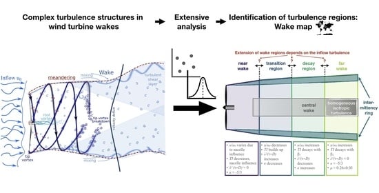
4]). As sketched in
Figure 1, the wake directly downstream of the turbine is determined by the presence of aerodynamic structures imprinted by the turbine (cf. [
2]): By conservation of momentum, the wake experiences a spin that is counter-rotating to the turbine’s rotation. From the blades, tip and root vortices are shed [
5], and they are transported downstream in the wake on a helical path. The root vortices are unstable and break down close to the rotor. The tip vortexes are more stable and surround the wake as a helical tip vortex sheet. Between the faster ambient flow and the slower wake, a thin shear layer is evolving and the wake is expanding. Eventually, the tip vortices break down, the shear layer expands, and the turbulent mixing process that fuels the wake recovery is started. The turbulence is building up until the shear layers meet in the middle of the wake. In the literature, the region close to the rotor where rotor-imprinted structures are present is called the
near wake, and it is said to extend up to two rotor diameters downstream. Then, the wake turbulence evolves in the
transition region towards the
far wake around five rotor diameters downstream. In the far wake, the velocity profile follows a Gaussian profile. Several wake models that address this region exist and can be used to estimate the mean velocity evolution (see e.g., [
4,
6]). From this brief overview, the complexity of the turbulence in the wake downstream of a wind turbine becomes clear.
The complexity is further increased by the variation of the inflow conditions in the atmosphere. For example, it was shown that a stronger turbulence in the inflow leads to a higher wake turbulence but also to a faster wake recovery. As a consequence, the question arises to what extent the extension of the wake regions and the wake evolution depend on the inflow conditions. To analyze the evolution of the turbulence in the wake of a wind turbine, different numerical and experimental studies both in the field and in the wind tunnel have been carried out. The first measure of turbulence is the turbulence intensity
that is defined as the ratio between the standard deviation
and the mean velocity
u of the flow,
. It can be shown that the turbulence intensity downstream of a turbine is higher than the turbulence intensity in the inflow. The wake
is therefore commonly modeled with the concept of “wake added turbulence” (e.g., [
8]; for different turbulence models of the wake, see also [
9,
10]). In [
11], the centerline evolution of the turbulence intensity is investigated with respect to the inflow turbulence by means of large eddy simulation up to 20 diameters downstream of the turbine. Here, it can be observed how the turbulence first builds up and then decays downstream, and how the position of the turbulence intensity maximum is dependent on the inflow turbulence intensity and the inflow velocity. As compared to the inflow turbulence intensity, the turbulence intensity in the wake is enhanced. This is also shown experimentally for example in [
12] in laminar inflow, and in [
13,
14] in an atmospheric boundary layer inflow.
Length scales characterizing the turbulence, especially the integral length scale
L, are another important parameter to study in wakes (see e.g., [
15,
16,
17]). On the one hand, it has been found that, when comparing the integral length scales in the near wake for laminar and turbulent inflow, the integral length scale is larger in the case of turbulent inflow. This can be interpreted as structures smaller than half the rotor diameter passing the rotor. On the other hand, as compared to the size of structures in turbulent inflow, the scales are reduced in the near wake which leads to the interpretation that larger structures are damped by the turbine.
Another way to analyze turbulent structures is by using the energy spectral density
. In particular, the tip vortices as well as their breakdown can be captured at radial positions
where
R denotes the radial position and
D the rotor diameter. The breakdown indicates the onset of wake recovery. The tip vortices can be captured up to normalized downstream distances of
2−3. They are more persistent under laminar inflow conditions, and their breakdown is accelerated by turbulent inflow (see e.g., [
15,
18,
19,
20]). Within the wake, energy spectra can reveal the interaction between the turbine and the inflow, which was for example done in [
16,
17,
21,
22,
23]. Depending on the inflow conditions it can be observed that the turbine either reduces turbulent structures larger than the rotor diameter while creating turbulence at scales smaller than to rotor diameter or reduces energy at high frequencies while increasing energy at small frequencies and thus larger flow structures.
In the framework of loads and also turbulence analysis, the intermittency plays an important role. Intermittency characterizes the “gustiness” of a flow or differently said the probability of sudden, large changes of the wind velocity. To identify intermittency, it is not sufficient to investigate one-point statistics like the mean velocity, standard deviation, or length scales. Instead, at least two-point statistics are necessary. However, only a few studies address the existence of intermittency in the wake of a wind turbine. In [
24], inter alia the role of the intermittency in the evolution of the wake turbulence is investigated. With regard to the intermittency in the inflow, references [
21,
23,
25] found that a turbine reduces intermittency in the flow. In addition, references [
21,
26] find indications of the existence of homogeneous isotropic turbulence in the wake. Reference [
27] finds that the wake is surrounded by a ring of high intermittency with approximately twice the rotor diameter downstream at
.
Overall, this brief overview motivates the detailed study of the turbulence evolution in the wake of a wind turbine and a wind turbine array, as many studies point out single effects at single downstream positions but the evolution of turbulence is rarely discussed from a turbulence perspective. The aim of this study is a systematic exploration of the evolution of the turbulence in the wake of a wind turbine to identify distinctive turbulence regions and create a map of the wake turbulence. In particular, if uniform criteria can be found, this will be a new tool for the analysis of wakes. For this, a detailed characterization of the turbulence in the wake is necessary, which has not been done before to this extent. In this paper, an extended analysis of the downstream evolution of turbulence within the wake of a turbine and a turbine array is thus carried out in a wind tunnel. The data will be analyzed by means of a classical turbulence investigation. One highlight is the high downstream resolution of measurement positions up to rotor diameter downstream of the turbine.
This paper will continue with a description of the experimental setup in
Section 2. Afterward, the results are presented in
Section 3 by extensively discussing the mean velocity, the variance, the turbulence intensity, the energy spectral density, the integral length scale and the Taylor length scale, and, finally, the shape parameter as a measure for intermittency. The results are discussed in
Section 4 and the paper ends with a conclusion in
Section 5.
2. Experimental Setup
In the following, the experimental setup that was used to carry out the study presented here will be explained. A sketch of the setup can be found in
Figure 2. The experiments were carried out in Oldenburg’s Large Wind Tunnel (OLWiT), a closed-loop wind tunnel that has an inlet of
and a closed test section of
length (cf. [
28]). Wind velocities of up to
can be achieved, and the background turbulence intensity is
. The wind speed is kept constant by closed-loop control. A uniform laminar inflow with a velocity of
was used during all experiments. This wind speed was chosen as the optimal turbine performance is achieved here. Two three-bladed horizontal axis model wind turbines of the same type have been used (cf. [
29]). The rotor blades are optimized for small wind turbines and have been manufactured using a vacuum casting method. Both turbines have a rotor diameter of
and a hub height of
. The blockage ratio in the wind tunnel is below 3% for a single turbine. The turbines are operated under optimal performance conditions with a tip speed ratio of
. For this condition, the thrust coefficient of the whole turbine was measured by placing the turbine on a force balance, and it is
(cf. [
30]). The thrust coefficient of the tower and nacelle was measured to be
. The turbines are controlled to optimize the power by using a closed-loop control that is run by a NI cRIO-9074 real-time system with a sampling time of 5 ms. For the control, a look-up table was created beforehand to link the rotor speed to the respective optimal torque reference (cf. [
31]).
Three wake scenarios have been investigated. First, only one turbine, turbine 1, was mounted centrally inside the wind tunnel. Measurements were taken at the hub-height in the wake downstream of turbine 1 between
and
in steps of
using an array of six 1d hot-wire probes whose positions can be found in
Figure 2. Afterward, a second turbine, turbine 2, was positioned
downstream of turbine 1 and thus centrally in the wake of turbine 1. Measurements were taken with the same 1d hot-wire array between
and
with respect to the rotor plane of turbine 2 in steps of
. Note that with respect to turbine 1, the measurement position the farthest downstream of turbine 2 is
which is a compromise between the same measurement
area downstream of both turbines (up to
with respect to turbine 1) and the same measurement
range (up to
with respect to turbine 2). This flow situation will be referred to as
turbine 2 mid. Finally, turbine 2 was shifted
to the side, thus being exposed to a non-uniform turbulent half-wake inflow situation which is often found in wind farms as well. The blockage in this case is below 5%. Similarly, measurements were taken between
and
with respect to the rotor plane of turbine 2 in steps of
. This flow situation will be referred to as
turbine 2 side. The hot-wires were operated using a StreamLine 9091N0102 frame with 91C10 CTA Modules from Dantec Dynamics (Skovlunde, Denmark). At each position,
data points were collected at a sampling frequency of
. The hot-wires were calibrated every four hours, and the flow temperature, the ambient pressure, and the humidity were monitored throughout the measurements to calculate the correct fluid properties and to apply a temperature correction according to [
32].
3. Results
In the following, the results obtained from the above-described measurements are presented. For this, first, the evolution of the mean velocity is investigated. Next, the evolution of the variance and the turbulence intensity are presented, followed by a discussion of the energy spectra. Afterward, the evolution of length scales within the wake is discussed, and finally, the intermittency is focused on. All quantities will be considered in the frame-work of turbulence regions in the wake.
3.1. Mean Velocity
In
Figure 3, the evolution of the mean velocity
u is plotted as an interpolated contour plot downstream of turbine 1 (
Figure 3a) and at the centerline with respect to the rotor position of the three respective turbine configurations (
Figure 3b–d). The mean velocity is normalized by the inflow velocity
. The interpolated contour plot enables an exemplary overview of the evolution of the whole flow field downstream of turbine 1. It can be seen how the velocity deficit downstream of the turbine recovers and the wake expands. The red dashed line indicates
which gives an idea of the wake width. At approximately
, this line shows a sudden jump due to the discretization caused by the rather coarse radial sensor spacing. The red dotted vertical line indicates the downstream position of turbine 2 and thus its inflow condition. A more detailed view of the evolution of the mean velocity is given by the centerline plots (
Figure 3b–d). For all wake situations, a small increase in the mean velocity is visible in the near wake directly downstream of the nacelle. This indicates an initial recovery of the nacelle’s lee as the flow is deflected similarly to the flow around a sphere or a cylinder. Then, the velocity decreases because the pressure that dropped across the rotor recovers to ambient pressure and the wake expands. Finally, the velocity recovery starts when due to turbulent mixing, the high-energetic ambient flow is entrained (see e.g., [
2,
33]; a similar evolution of the mean centerline velocity is found in [
34]). While the evolution of the three measured wakes is similar, the influence of the inflow turbulence is directly visible (cf.
Table 1): In the laminar inflow downstream of turbine 1, the wake recovery starts from
downstream of the rotor while both turbulent inflows accelerate the recovery significantly: Downstream of turbine 2 mid, the recovery starts from
, and downstream of turbine 2 side, the recovery starts from
.
Already from the simple consideration of the centerline mean velocity evolution, one can identify downstream regions in the wake, first, the near wake region where the nacelle influence is present, second a region where the velocity decreases, and third the region where the velocity recovers. At the end of the respective measurement regions, the velocity has recovered to 70% of the inflow velocity.
3.2. Variance
Next, the downstream evolution of the variance
at the centerline will be discussed. The results are plotted in
Figure 4a–c for the three turbine configurations. Just as for the evolution of
, we find that the development of
follows the same sequence as a function of downstream direction for the three cases considered here. In the near wake, the variance decreases (cf.
Figure 4a–c) due to the mixing of the turbulent wake of the nacelle and the root vortices shed from the blades with the low-turbulent turbine wake flow in the vicinity of the rotor. Next, the variance increases when the turbulent mixing due to the expanding shear layer surrounding the wake starts, and turbulence builds up. Finally, the variance diminishes when the shear layers surrounding the wake have merged and the turbulence starts to decay in the far wake. The positions of the local minima and maxima are indicated in
Table 1. As can be seen, the area around the maximum resembles a plateau. Therefore, to define the downstream position from which the decay starts, a polynomial fit of 12th order was used to fit the curves. Polynomial fits of different order have been tried and a fit of 12th order was chosen to have a good interpolation in the rather flat area around the local maxima. The first derivative was used to find the maximum
(full vertical line). In addition, the point of maximum curvature
upstream of the maximum was found using the second derivative (dashed vertical line). The plateau is defined as a symmetric region around the maximum,
, as indicated by the dashed and the dash-dotted line, and the decay starts from the dash-dotted line. When investigating the turbulence intensity in the next section, the reason for this procedure will become clear.
3.3. Turbulence Intensity
After briefly discussing the variance, the turbulence intensity , that connects the mean velocity u and the variance , will be investigated. It gives a measure of the strength of the fluctuations with respect to the flow velocity.
Figure 5a shows an interpolated contour plot of the downstream evolution of the turbulence intensity in the wake of turbine 1. The dashed red line gives an approximation of the wake boundary at
. From this plot, the wake expansion can be seen as outside of the wake, the flow is laminar and inside the wake, the turbulence levels are significantly higher due to the turbine adding turbulence. Inside the wake, two areas with very high turbulence levels can be distinguished, one being directly downstream of the rotor in the nacelle’s lee and the other being around
. To investigate this in more detail, the evolution of the centerline turbulence intensity is plotted in
Figure 5b–d for the three inflow conditions. Downstream of the turbines, the turbulence intensity first drops in the near wake similarly to the variance. Then, it builds up in the region where the shear layers expand and fuel turbulence production. Finally, the turbulence intensity decays. The exact downstream positions of the local minima and maxima are indicated in
Table 1. Again, the three wakes behave in principle similarly but an influence of the inflow turbulence on the evolution is present both with respect to the downstream position of the maximum and with respect to the maximum of the turbulence intensity (cf.
Table 1). The downstream position of the maximum turbulence intensity differs from the position of the maximum variance. The turbulence intensity maximum downstream of turbine 2 mid is the largest which is expected as, in this situation, the turbine is exposed to a fully turbulent inflow situation, while turbine 2 side is exposed to a half-wake inflow and, thus, averaged over the whole flow field to less turbulence (but stronger velocity gradients). In addition, the turbulence decays faster with increasing ambient turbulence, which is also expected from the literature (e.g., [
11]).
Similarly to the results obtained from the mean velocity and the variance, one can identify regions by means of the turbulence intensity, i.e., the drop in the near wake, the build-up in the transition region, and the decay in the far wake, and again, the extension of the respective regions depends on the inflow turbulence.
The decay of the turbulence intensity can be investigated more intensively in analogy to the decay of turbulence downstream of for example grids. In turbulence research, the decay region is often assumed to follow a power law which indicates the self-similarity of the turbulence (e.g., Ref. [
35] for turbulence in general; e.g., Ref. [
8,
14] for self-similarity of wake profiles of wind turbine wakes). Therefore, a power law fit according to
is applied to the data. Interestingly, it is especially clear in the case of the turbulent inflow conditions that the slope is changing from the beginning of the decay region to the end of the measurement region. For that reason, the fit region was split into two parts, one where the decay begins and one where the decay process has changed. As the two vertical lines indicate, the decay of the turbulence intensity starts with the start of the plateau in the variance curves (cf.
Figure 4), and the exponent changes where the variance starts to decrease (dash-dotted line). The decay exponents can be found in
Table 2. This indicates the existence of a fourth downstream region with respect to the turbulence. A similar behavior can also be found downstream of regular grids where the turbulence decay process also changes [
36].
3.4. Energy Spectral Density and Decay Exponent in the Inertial Sub-Range
After presenting the evolution of the mean velocity, the variance, and the turbulence intensity, the energy spectrum will be analyzed in dependence on the downstream position and also with respect to the radial position. By means of energy spectra, periodic structures like the tip and root vortices can be identified on the one hand while on the other hand, conclusions can be drawn about the turbulence.
In
Figure 6, the downstream evolution of energy spectra is plotted for the three scenarios and two lateral positions, namely the centerline
and the blade tip position
. The downstream position is indicated by color coding where a brighter color indicates a position farther downstream. In addition, the spectrum of the inflow generated by turbine 1 is plotted for turbine 2 at the position of the rotor center (dark red dash-dotted lines) and at the last measurement position (red dashed lines).
When looking at the centerline evolution downstream of turbine 1,
Figure 6a, the root vortex is identifiable close to the rotor up to
and the turbulence level in small scales is high due to the vortices shed from the nacelle. With increasing downstream position, the energy in small scales first drops up to
where the turbulent vortices shed from the blade roots and the nacelle mix with the low-turbulent turbine wake flow directly downstream of the rotor. When the shear layers expand and fuel turbulent mixing, the energy spectral density increases. A similar effect can be seen for the large scales (≳D) in a less pronounced manner. From approximately
downstream, the turbulence is fully developed, and the spectra collapse and show an inertial sub-range that follows a decay according to
. Looking at the evolution of energy spectra downstream of turbine 2 mid,
Figure 6c, it can be seen that close to the rotor, the spectrum is similar to the spectrum of the inflow because most of the structures from the inflow pass the rotor. With increasing downstream position, the energy increases both in large and in small scales, and the spectra collapse again to one spectrum that is also similar to the spectrum downstream of turbine 1. The spectra appear to follow a decay according to
. Downstream of turbine 2 side,
Figure 6e, the evolution resembles the evolution downstream of turbine 1 with a drop in energy at small scales, followed by an increase towards one unique spectrum. The unique spectrum shows again a decay according to
and is similar to the behavior downstream of turbine 1. The large scales do not evolve and are similar to the turbulent inflow in the shear layer of turbine 1. This indicates that they are transferred to the wake.
At the position of the blade tip,
, the downstream evolution of the energy spectral density in
Figure 6b,d,f is shown to be similar to the evolution at the centerline a convergence towards one unique spectrum that decays in the inertial sub-range according to
for all cases. This is illustrated in
Figure 7 where the spectra of the respective last measurement position are plotted for the three scenarios and the three radial positions
,
, and
. For a better comparison, in
Figure 7a, the spectra are normalized by the energy at
so that they collapse, and in
Figure 7b the original spectra that have small differences in the energy are shown. While the spectra at all radial positions and for all cases are nearly identical in the far wake, the evolution of the turbulence itself is different as at the outer radial position, aerodynamic effects are present close to the rotor. In the spectra of turbine 1 and turbine 2 side, the peaks in the spectrum indicate the tip vortices and their harmonics. Downstream of turbine 2 mid, they are not captured due to the high ambient turbulence level at the blade position that causes a quick breakdown.
From this discussion, it can be concluded, that there is a difference between the wake core and the outer wake, and that far downstream, the turbulence generated by the turbine is dominating and creates turbulence with one unique spectrum.
To characterize the decay of the energy spectra at the centerline more thoroughly,
Figure 8a–c shows the evolution of the decay exponent
of the energy spectral density in the inertial sub-range for the three scenarios. For the determination of
, a fit according to
is applied to the inertial sub-range. It can be seen that close to the rotor,
. Then,
decreases, increases again, and tends towards
which is very close to the expected value of
[
37].
Similarly to the above-discussed quantities, namely the mean velocity, the variance and the turbulence intensity, wake regions can be identified by means of the energy spectra: From the downstream evolution of the decay exponent, four regions can be identified at the centerline that indicates the evolution of turbulence towards a decay. In addition, the radial downstream evolution is different which indicates the existence of a wake core and an outer region with respect to the turbulence.
3.5. Integral Length and Taylor Length
The inertial sub-range of an energy spectrum is not only characterized by the decay exponent
but also by the frequency range where this decay is found. This range is limited by the integral length scale
L at low frequencies and the Taylor length
at high frequencies. Both quantities are calculated from the one-dimensional energy spectrum as suggested by [
36] and explained in [
30].
Figure 9 shows the evolution of the integral length as interpolated contour plot downstream of turbine 1 (
Figure 9a) and the centerline evolution downstream of turbine 1, turbine 2 mid, and turbine 2 side (
Figure 9b–d). From the interpolated contour plot, it can be seen that the integral length directly downstream of the rotor is small because the rotor filters larger structures. It increases when the wake and its turbulence evolve downstream and larger turbulent structures are transported into the wake. Also, the integral length in the wake increases from the centerline towards outer radial positions from
, while outside of the wake (the dashed
line gives an approximation of the wake boundary), the integral length is smaller.
The increase of the integral length downstream at the centerline is emphasized for all wake scenarios in
Figure 9b–d. While the integral length increases downstream of turbine 1 first slowly and from
faster, it increases downstream of turbine 2 quicker in the same downstream region because of the stronger turbulence. At the end of the respective measurement range, the integral length is similar for all scenarios and has a value of approximately
.
In
Figure 10, the downstream evolution of the Taylor length
at the centerline is plotted for the three wakes in (a)–(c). Downstream of turbine 1 (
Figure 10a), the Taylor length increases from
at
up to
at
. This indicates decaying turbulence in the region close to the rotor where the vortices shed from the nacelle decay and mix. Then,
drops where the turbulence builds up, and it finally increases again from
in the far wake where the turbulence decays. Downstream of turbine 2 mid, the evolution is similar but the maximum is closer to the rotor. Downstream of turbine 2 side, the Taylor length increases but without a pronounced maximum. At the end of the measurement range,
for all scenarios.
3.6. Castaing Parameter
By means of the Castaing parameter
, the intermittency, or “gustiness”, within the wake is discussed. This intermittency, known from homogeneous isotropic turbulence, can not be identified by means of one-point statistics but has to be investigated with two-point statistics. Therefore, the central velocity increment
with respect to the time scale
is defined. Then, the Castaing parameter can be calculated from the flatness F of the velocity increments [
38],
By this definition, the Castaing parameter
is calculated from higher-order two-point statistics. It is also sometimes called the shape parameter as it describes the whole shape of the probability density function
. In contrast to the shape parameter, the energy spectrum contains the second-order two-point statistics of
, and thus the dependence on the scale
solely indirectly by means of the variance of
as the energy spectrum is related to the autocorrelation function by the Wiener–Khintchine theorem [
39]. Thus, the combination of the energy spectrum that gives the variance of
and the Castaing parameter
represents a complete statistical two-point characterization in terms of velocity increments (cf. [
40]). Structure functions of all orders which are commonly used for turbulence analysis are fully captured by this analysis.
The Castaing parameter is also a measure of the deviation of the probability density function of the velocity increments from a Gaussian distribution.
indicates a higher probability of large changes in the velocity increment as compared to a Gaussian distribution, and this is characteristic of intermittency. It has been shown by [
41,
42] that taking into account the intermittency at time scales corresponding to the rotor diameter
D is important to prevent an underestimation of the fatigue loads.
In
Figure 11, the Castaing parameter
is plotted with respect to
as interpolated contour plot downstream of turbine 1,
Figure 11a, and at the centerline downstream of turbine 1, turbine 2 mid, and turbine 2 side in
Figure 11b–d. The evolution of
downstream of turbine 1 (cf.
Figure 11) shows that within the wake,
except for a small region around
. Noticeable is that directly outside of the wake that is indicated by a line marking
, a region of high intermittency is found to surround the wake. In [
27], it has been discovered for the first time that the wake is enveloped by a ring of high intermittency at
, and this ring is tracked over the whole flow field in the measurements presented here.
The vertical red dotted line in
Figure 11a indicates the position of turbine 2, and it can be seen that the inflow conditions in the case of turbine 2 mid are non-intermittent while turbine 2 side is exposed to an inflow with high intermittency at one half of the rotor and low intermittency at the other half of the rotor, emphasizing the complexity of this inflow condition.
In
Figure 11b–d, the centerline evolution of
is shown for the three inflow scenarios. For all scenarios,
directly downstream of the rotor in the near wake. Then,
increases up to
when the turbulence builds up in the transition region and decreases again, tending towards
again in the far wake at the end of the measurement range. While the evolution is similar, the downstream region in which the local maximum is found varies for the three scenarios. Also, before tending to
, the Castaing parameter falls below 0 to
in the case of turbine 2 side, which indicates that the probability density function of velocity increments is sub-Gaussian. The evolution of the Castaing parameter indicates similarly the existence of four wake regions as already demonstrated above.
Last, the evolution of the Castaing parameter over the time scale
is discussed for the far downstream position, for which we postulated above a universal turbulence behavior.
Figure 12 shows the evolution of the Castaing parameter across the time scale
with logarithmic abscissa at the respective last measurement position for the three inflow scenarios. For all scenarios,
decreases to
at
. By means of Taylor’s hypothesis [
43], the corresponding length is found to be
which is indicated by the vertical dashed line. Intermittency is therefore induced in the far wake of a wind turbine for scales smaller than half of the rotor diameter but filtered for scales larger than the rotor diameter. The decrease can be characterized using Kolmogorov’s theory for the scaling behavior of the structure functions in the case of fully developed turbulence (see e.g., [
44]),
is the intermittency parameter, and it can be used to identify homogeneous isotropic turbulence in the flow. In the case of homogeneous, isotropic turbulence,
is found in the literature (see e.g., [
44]).
In
Figure 12, a fit according to Equation (3) was applied to the data, and the values found for the intermittency parameter are
for turbine 1,
for turbine 2 mid, and
for turbine 2 side. Therefore, together with the results obtained from the analysis of the energy spectra, we conclude that the behavior of turbulence in the far wake of a wind turbine follows the theory for homogeneous isotropic turbulence with intermittency. This observation is independent of the inflow, particularly the intermittency in the inflow.
4. Discussion
We have presented an experimental investigation of the evolution of turbulence within the wake of a wind turbine exposed to laminar inflow as a reference case and two different wake inflow scenarios. The mean velocity, variance, turbulence intensity, integral length, Taylor length, energy spectra, and Castaing parameter have been investigated with the aim of identifying turbulence regions that occur independently of the inflow condition. It was shown that four downstream regions, a wake core, and an intermittency ring can be distinguished in all three scenarios. Not all regions are equally recognizable by the different quantities but as an ensemble, they give a good indication of the regions. In
Figure 13, the regions are visualized and summarized in a “wake map”. Directly downstream of the rotor, the mean centerline velocity varies due to the influence of the nacelle and decreases in the near wake. The variance and the turbulence intensity decrease in the nacelle’s wake that mixes with the low-turbulent flow close to the rotor. Intermittency is not present at scales related to the rotor diameter (
), and the decay exponent
of the inertial sub-range is approximately
. The Taylor Reynolds number indicates not fully developed turbulence,
where
denotes the kinematic viscosity of air. Then, the turbulence starts to build up in the transition region where the tip vortices start to break down and the shear layers expand: The mean centerline velocity decreases while the variance and the turbulence intensity increase, the decay exponent
decreases, and intermittency at scales related to the rotor diameter builds up at the centerline. Next, where the shear layers meet, the mean centerline velocity starts to recover, the variance changes slowly as it reaches its maximum and the turbulence intensity starts to decay in the newly introduced
decay region. Here, the turbulence intensity decays according to a power law with a decay exponent
. The decay exponent
of the energy spectrum increases again while the intermittency decreases. Finally, in the far wake, the turbulence is fully developed. The mean centerline velocity increases, the variance decreases, and the decay of the turbulence intensity changes from a power law with exponent
to a power law with exponent
. The energy spectra collapse and the inertial sub-range follows a decay close to
. The integral length and the Taylor length increase and their ratio is constant which indicates an inertial sub-range whose extension remains constant despite the decaying turbulence. The Taylor Reynolds number indicates fully developed turbulence,
. This is also supported by an estimation of the intermittency parameter
from the evolution of the Castaing parameter across the scales
in the far wake. The determined value of
fits perfectly the expected value for fully developed homogeneous isotropic turbulence of
given in [
44]. In addition, the wake is surrounded by a ring of high intermittency at scales related to the rotor diameter.
Overall, four downstream regions were identified by means of centerline turbulence quantities for three relevant inflow cases, and their extension was discussed in detail thanks to the high downstream resolution of measurement points. The extension of the respective regions depends on the inflow turbulence, but the turbulence in the wake of a wind turbine evolves similarly independently of the inflow conditions. Therefore, we found uniform criteria to describe the wake which can be a tool for the analysis of the wake only by means of the centerline. From these measurements, we can give a first rough estimation of the extension of the wake regions. In the case of laminar inflow, the near wake extends to roughly
, the transition region extends approximately between
and
, the decay region is found between
and
, and the far wake starts around
. In the case of turbulent inflow, the near wake extends to approximately
, the transition region is found between
and
, the decay region between
and
, and the far wake from approximately
. A comparison with the plots of
u and
shown in [
45] gives a similar estimation of the regions for the cases with lowest and highest inflow turbulence, respectively.
The results allow the interpretation that the turbine imprints its own turbulence onto the wake that always tends towards homogeneous isotropic turbulence in the far wake. The energy spectra collapse to one unique spectrum, and in contrast to the interpretation in [
16], we believe that the turbine does not act as an active filter that diminishes large and very large scales while enhancing the energy in small scales but that the turbine does generate its own turbulence that shows with respect to the inflow turbulence a unique spectrum that this has more or less energy in high frequencies as compared to the inflow. In the far wake, intermittency is present up to scales corresponding to approximately half the rotor diameter. For scales corresponding to the rotor diameter, intermittency is not present in the central far wake independently of the intermittency in the inflow. However, in the transition and decay region, intermittency at scales
can be identified, and additionally, intermittency is present in a ring surrounding the wake in all wake regions. These results are important as [
42] could show that a flow with intermittency for scales
induces higher fatigue loads at the rotor blade than a flow where intermittency is neglected.
5. Conclusions
In this paper, we presented a study of the small-scale turbulence in the wake of a wind turbine exposed to three different inflow scenarios, namely laminar inflow, a central wake from an upstream turbine and a half-wake from an upstream turbine. By means of the mean velocity, variance, turbulence intensity, energy spectra, integral length and Taylor length, and the Castaing parameter, the downstream evolution of the turbulence was discussed. Our aim was to identify characteristic turbulence regions that exist independently of the inflow conditions to introduce a new way of looking at wakes. Four downstream wake regions whose extension depends on the inflow turbulence could be identified in all scenarios by means of an investigation of the centerline only. In addition, radially, a wake core with features of homogeneous isotropic turbulence and a ring that surrounds the wake along the whole measurement region were identified. We therefore found uniform criteria to describe the wake turbulence. The results have been summarized in a turbulence wake map which gives a new tool to investigate wind turbine wakes. The results lead to the interpretation that a wind turbine generates an own, dominating turbulence that overwrites the signature of the inflow turbulence. This finding is based on a comprehensive data analysis showing that the energy spectra as well as the intermittency quantified by the Castaing parameters collapse to unique scale dependencies in the far wake. Additionally, the results indicate that double- and multi-wake scenarios in a wind farm do not increase the complexity of the turbulence at least in this far wake region - for these wakes, only the relative positions of the different regions have to be found. If, for example, the same energy spectra of a single wake are found in the double wake situations (see
Figure 7), it is likely that the same holds for multiple wakes. Although the aim of the paper is not to present a new wind farm design, the results are of interest for the optimization of wind turbine spacing in wind farms because the new way of wake characterization in wind farms may become useful for advanced methods of farm design in the future.
The high downstream resolution of measurement positions enables a detailed examination of the evolution of the respective quantities. It has to be pointed out that a comparison of the wakes in different inflow conditions at solely one position or with a coarse spacing is insufficient as measurements from different turbulence regions could be compared, which would result in a biased interpretation.
The results encourage an analysis of the downstream evolution of the wake also with different inflow velocities and tip speed ratios to further extend the wake map. A possible application is the active control of turbulence regions by means of the turbine control to reduce loads on downstream turbines and enhance turbulent mixing and thus the wake recovery.

 ,
, 


