Abstract
A NILM dataset is a valuable tool in the development of Non-Intrusive Load Monitoring techniques, as it provides a means of evaluation of novel techniques and algorithms, as well as for benchmarking. The figure of merit of a NILM dataset includes characteristics such as the sampling frequency of the voltage, current, or power, the availability of indications (ground-truth) of load events during recording, the variety and representativeness of the loads, and the variety of situations these loads are subject to. Considering such aspects, the proposed LIT-Dataset was designed, populated, evaluated, and made publicly available to support NILM development. Among the distinct features of the LIT-Dataset is the labeling of the load events at sample level resolution and with an accuracy and precision better than 5 ms. The availability of such precise timing information, which also includes the identification of the load and the sort of power event, is an essential requirement both for the evaluation of NILM algorithms and techniques, as well as for the training of NILM systems, particularly those based on Machine Learning.
1. Introduction
Non-Intrusive Load Monitoring (NILM) techniques are under development, globally, as part of the effort to improve Electrical Energy Efficiency. To support this development, specific datasets have been elaborated, particularly during the last decade. A NILM dataset consists of a collection of samples taken over time; these may include voltage, current, active power, and reactive power. As NILM techniques concern disaggregation of loads, typically, the samples in a NILM dataset comprise aggregated current and power.
According to the International Energy Agency [1], the worldwide electricity demand is currently 29,000 TWh and will increase to 42,000 TWh in 2040 at about 2.1% per year. Under current Stated Policies, less than 50% of this energy will come from renewable sources: mainly solar, wind, and hydro. Improvements in this scenario may be attainable by reducing waste and improper use, as well as reducing the electrical energy needs, mainly by improving the efficiency of electrical devices. Hence, the importance of Electrical Energy Efficiency, which aims at the reduction in power and energy demands of electrical systems without affecting their functionality. Most importantly, reducing energy needs has a significant effect on the environment by reducing the world’s carbon emissions.
NILM techniques are based on a centralized measurement of electrical energy consumption and, through a disaggregation process, determination of the individual consumption of each electrical load. Typically, NILM uses a database of known power signatures of devices to analyze the aggregated power consumption and identify the contribution of each load. Therefore, NILM is a low-cost, easily deployed, flexible, and, therefore, viable solution that provides consumers with detailed information about their energy consumption [2]. NILM provides essential information for use in Smart Grids, in Energy Management Systems, and for Energy Efficiency initiatives.
The rationale for a NILM dataset is fivefold:
- A dataset provides a stable set of input data that can be used to compare the performance of different solutions. As such, research under development by different groups can be compared over the same conditions.
- Collecting data for a dataset requires a significant amount of effort and time. Making a dataset publicly available is a means of supporting researchers globally and accelerating results.
- The development of new NILM techniques requires a thorough understanding of the problem domain. A comprehensive NILM dataset provides support for such an understanding.
- As new NILM techniques and algorithms evolve, performance must be compared incrementally. A dataset provides a framework for consistent comparisons as well as for debugging.
- NILM datasets can be used for training, i.e., to feed event identification and load classification methods to build an initial signature database that is key to many NILM techniques.
To support our ongoing research on a NILM solution [3] a dataset with particular requirements was needed. Since the available NILM datasets did not match these requirements, we decided to pursue the development of a new dataset [4], named after our laboratory, by using an engineering development process starting with requirements elicitation. During this development, a testing jig was constructed to allow recording in a framework where up to eight loads could be individually controlled (turned on or off) and register their waveforms (samples of voltage and current) in a controlled load shaping scenario, named Synthetic load shaping subset. Power detection devices were also built and connected to each load, in a residential or research lab environment, to provide precise event records in a scenario of recording in a real (thus, not-controlled) environment (this subset was named Natural load shaping). To these two subsets, a third one was added, consisting of Simulated loads. In this case, scenarios that are hard to obtain in the real world, such as short circuits, can be included.
The taxonomy of NILM datasets may be organized by (1) sample frequency with low-frequency being up to 1 Hz and high-frequency when above that [5]; (2) the event-aware datasets being those that register the occurrence of each load event, while the event-free datasets do not; and (3) the presence (or not) of ground-truth information, either by indicating which loads caused each event or by registering the individual consumption of each load over time. The LIT-Dataset samples voltage and aggregated current at 15 kHz (256 samples per 60 Hz-mains cycle); records single and multiple concurrent loads and registers each load event to provide ground truth.
The organization of the following sections is as follows: Section 2 describes the publicly available datasets; Section 3 lists the requirements for the proposed dataset; Section 4 describes the three subsets that compose the LIT-Dataset: synthetic load shaping, simulated loads, and natural load shaping; Section 5 presents and analyses the results obtained, and Section 6 presents the conclusions to the work presented here.
Previous Research Contributions
The LIT-Dataset has been developed under an ongoing research project, funded by COPEL and ANEEL. Previous publications and patent requests, resulting from this research project, are listed in Table 1.

Table 1.
Related publications from the same research project.
Three of the publications listed in Table 1 concern the LIT-Dataset, presenting preliminary results. In [9], the dataset proposal, jig’s design, and initial results for the Synthetic Subset were presented, emphasizing the control mechanism for load switching and the acquisition circuit with its respective instrumentation. In [10], subsequently, the initial results with Simulated Subset were discussed, demonstrating the validation of load models and the automation procedure for generating waveforms. Finally, in [13], the architecture for a Natural Subset was presented, with a focus on the low-cost proposal of a time synchronization mechanism among nodes.
The other publications [3,6,7,8,11,12] detail the power signature analysis methods proposed in the same research project, using the LIT-Dataset and other recent datasets presented in the literature. Particularly in [3], a multi-agent architecture was presented and validated for event detection, feature extraction, and load classification, using different publicly available datasets. Some of the results were only possible due to the original features of the proposed LIT-Dataset. For instance, agents trained in a single load scenario and tested in another scenario with multiple concurrent loads were only possible because the LIT-Dataset includes such waveforms with single loads and different load combinations. A sample-level comparison for event detection was also only feasible due to the accurate labeling of the LIT-Dataset. This precise annotation of occurrence of each event is also primordial to allow the extraction of transient features from waveforms during the training stage, and, consequently, make use of the different feature extraction agents proposed in that work.
2. Related Work
The subject of the NILM dataset can be placed in the broader area of energy-related datasets and the associated means of data sensing and recording. Concerning data acquisition technologies, according to [14], there are five technologies classes employed to gather data and associated modeling methodologies: (1) energy consumption quantification, based on electricity meters; (2) indoor environmental measurements, based on ambient sensors, e.g., temperature, humidity, CO2 concentration, among others; (3) occupant behavior statistics that are estimated using cameras, Passive InfraRed (PIR) sensing, and similar sensors; (4) status sensors, including doors and windows status readers; (5) others, combining different elements, as Radio Frequency IDentification (RFID) or Ultra Wide Band (UWB) sensors.
Concerning NILM datasets and NILM systems, electrical energy data is usually collected directly by low-cost voltage and current sensors. In [15], voltage AC sensors, Hall-effect based current sensors, and analog-to-digital converters were employed for load monitoring purposes. With respect to the communications infrastructure, [15] employed Ethernet, while [16] used a 433 MHz wireless sensor network gathering AC voltages and currents from individual devices.
A taxonomy for datasets of power consumption in buildings is presented in [17]. On a first level, datasets are classified as Appliance Level versus Aggregated Level. An Appliance Level dataset contains individualized information of energy consumption of every appliance, while an Aggregated Level dataset contains aggregated power consumption data of a whole residence or building. On a second level, seven application purposes are listed: energy savings, appliance recognition, occupancy detection, preference detection, energy disaggregation, demand prediction, and anomaly detection. A survey with 32 datasets is presented, comparing their characteristics and application purposes.
In the following sections, NILM datasets described in the literature are presented in two classes: (1) low-frequency datasets (sampling frequency up to 1 Hz); (2) high-frequency datasets.
2.1. Low-Frequency Datasets
The following low-frequency datasets were analyzed and compared: Smart [18], HES [19], Tracebase [20], DataPort [21], AMPds [22], iAWE [23], GREEND [24], REFIT [25], and RAE [26].
The relevance of these datasets is due to the characteristics of the installed measuring devices. However, many of the possible strategies for feature extraction, that can be used for NILM classification, are restricted due to low sampling frequency.
A comparison between some characteristics of the different types of low-frequency NILM datasets can be seen in Table 2. Where represents the sampling frequency; DCD stands for Data Collection Duration; NoC corresponds to Number of Appliance Classes; NoA represents the Number of Appliances; and Res., Lab., Com. and Ind. are short forms for: Residential, Laboratory, Commercial and Industrial installations, respectively. Since the sampling occurs at very low rates (once a minute to once a second) the recordings can take place for very long times (weeks to years).
Table 2.
Comparison between low-frequency Non-Intrusive Load Monitoring (NILM) datasets.
2.2. High-Frequency Datasets
The following high-frequency datasets were analyzed and compared (Table 3): REDD (Reference Energy Disaggregation dataset), BLUED (Building-Level fUlly-labeled dataset for Electricity Disaggregation), PLAID (Plug Load Appliance Identification Dataset), HFED (High-Frequency Energy Data), UK-DALE (United Kingdom recording Domestic Appliance-Level Electricity), COOLL (Controlled On/Off Loads Library), SusDataED (Sustainable Data for Energy Disaggregation), WHITED (Worldwide Household and Industry Transient Energy Dataset), BLOND (Building-Level Office enviroNment Dataset), and SynD (Synthetic energy Dataset).
Table 3.
Comparison between high-frequency NILM Datasets.
REDD [27] is a residential dataset intended for research on disaggregation methods. REDD contains measurements from 6 different houses obtained over several months. The house input AC mains voltage and aggregated current are monitored at a sample rate of 15 kHz. Furthermore, the voltages and currents at individual circuits are monitored at a sample rate of 0.5 Hz, and plug-level monitors at a sample rate of 1 Hz. Similar to several of the datasets analyzed here, REDD provides ground truth data by presenting energy samples of individual appliances (monitored at plug-level) and of subsets (monitored at circuit level) of the total load.
Similarly, BLUED [28] is a dataset obtained from a single-family residence. This dataset registers the AC mains voltage and aggregated current. The sampling rate is 12 kHz, and the measurements were performed for 1 week. Every state transition of the 43 appliances is labeled and time-stamped, providing ground truth for event detection algorithms.
PLAID [29] is a public and crowd-sourced dataset consisting of one-second voltage and current waveforms for different residential appliances. The goal of this dataset is to provide a public library for high-frequency (30 kHz) measurements that can be integrated into existing or novel appliance identification algorithms. PLAID currently contains measurements for more than 200 different appliances, grouped into 11 appliance classes, and totaling over a thousand records.
UK-DALE [16] is a publicly available dataset comprising records from 5 different houses. It contains AC mains voltage and aggregated current, as well as voltage and current of individual loads, hence, providing ground-truth for testing disaggregation and training algorithms. The sampling rate is 16 kHz for the house input, while the individual sensors are sampled every 6 s. There are more than 4 years of data in this dataset and it is continuously updated.
HFED [30] is a high-frequency Electromagnetic Interference (EMI) dataset comprising high-frequency measurements of EMI, emanated from electronic appliances, propagated through the power infrastructure, and measured at a single point. HFED includes 24 appliances connected over four different test setups (in lab settings and one test setup in home settings). EMI measurements are taken over a frequency range of 10 kHz to 5 MHz.
COOLL [31] is a publicly available home appliance dataset containing 42 appliances grouped into 12 classes. The AC mains voltage and current are monitored for each appliance at a sample rate of 100 kHz for 6 s, which includes turn-ON and turn-OFF transients. For each appliance, there are 20 measurements on different power-on angles of the mains cycle. Each appliance is measured individually; hence, there is no aggregated current data registered in the dataset.
SusDataED [32] is an extended version of the dataset SusData [33]. This dataset is composed of measurements taken from a single-family residence in Portugal. Samples of 17 distinct appliances were taken at a sampling rate of 12.8 kHz for ten days.
WHITED [34] is a dataset of appliance measurements from several locations (households and small industries) around the world. The voltage and current waveforms are recorded with the first 5 s of the appliance start-ups for 110 different appliances, amounting to 47 different appliance types. This dataset aims to provide a broad spectrum of different appliance types in different regions around the world.
BLOND [15] is a dataset with waveforms collected at a typical office building in Germany. It is a fully-labeled ground truth dataset, with 53 appliances distributed in 16 classes of devices, sampled at 50 kHz during 213 days.
SynD [35] is a synthetic dataset composed of residential loads. This dataset is the result of a 180 days custom simulation of a residential environment that relies on power traces of real household appliances. SynD is composed of measurements taken from 21 appliances in Austria, with a sampling rate of 5 Hz, during 180 days.
Table 3 shows a comparison between these high-frequency NILM datasets. It includes information on the environment (if data was collected in a Residential, Commercial, or Industrial environment); the Duration of the period of Data Collection (DCD); if the dataset includes scenarios of Multiple Simultaneous Loads (MSL); the sampling frequency (); if Ground Truth is recorded, either as the recordings of current/power of individual loads or as recordings of events (at a given Load Event Resolution—LER); the Number of Appliance Classes (NoC); and the Number of Appliances (NoA).
2.3. Evaluation of Datasets
The analysis of the datasets, both high-frequency and low-frequency, presented above indicates that: (1) the majority of NILM datasets contains data collected in a residential environment; (2) the majority of high-frequency datasets register 200 or more samples per mains cycle, a notable exception being SynD whose sampling frequency is 5 Hz; (3) the majority of the datasets register multiple simultaneous loads. Concerning the unique characteristics of each dataset it can be observed that: (1) the‘highest sampling frequency is used by COOLL (100 kHz); (2) while most low-frequency datasets do not provide ground-truth information, the high-frequency datasets provide ground truth by recording at a much lower rate (typically bellow 1 Hz) samples for individual loads.
2.4. Tools for NILM Datasets
The NILM Toolkit (NILMTK) [36] is an open-source toolkit designed to allow the comparison between NILM algorithms. It provides a Python API that operates on input and output binary files, therefore facilitating compatibility with data from NILM datasets. The input files used by NILMTK must be converted to the NILMTK-DF (data format), which is a data structure inspired on the dataset REDD comprising disaggregated power data (i.e., separate sample sets for each of the loads in a dataset) as well as metadata annotations about the sample set.
3. The Design of a Novel Dataset
Since none of the evaluated datasets had all the required characteristics for our research project, a new dataset development took place, with the first activity being requirements elicitation.
The LIT-Dataset is composed of three subsets: Synthetic, Simulated, and Natural. The Synthetic subset is obtained by a programmable power sequencing to a given set of loads in a controllable laboratory setup, so that repeatable scenarios can be obtained. In the Simulated subset, data is collected by simulating a circuit operation, allowing to test different scenarios and to control parameters that otherwise would not be possible or would be unsafe. The Natural subset is composed of voltage and current samples collected in a real-world uncontrolled environment; furthermore, apart from recording the aggregated current and the AC mains voltage, power sensors monitoring each load identify and record when each load event occurs.
Concerning the taxonomy presented in [17], the LIT-Dataset is an Aggregated Level dataset whose main application is Energy Disaggregation but is also applicable to energy saving, appliance recognition, and anomaly detection.
One of the requirements of the LIT-Dataset is that it includes multiple loads, as a NILM system must identify the loads that compose an aggregated current signal. Another requirement is that it must include precise indications of every load event (load on and load off), with a resolution better than one mains cycle, and have a high sample rate.
The Stakeholder requirements of the LIT-Dataset are based on the needs of the authors’ NILM project, as well as on the requirements common to other NILM datasets. The LIT-Dataset Stakeholder requirements are listed below, as well as the rationale for each requirement:
- DSReq 1.
- Data collection from loads connected to a single-phase 127 V, 60 Hz mains (the Brazilian power grid standard).R: Due to power grid availability in our lab. Considering that 127 V, 60 Hz, is a standard used in many countries around the world, such a requirement does not restrict the usage of the LIT-Dataset elsewhere.
- DSReq 2.
- Comprised of residential, commercial, and low-voltage industrial loads.R: A NILM dataset should include a variety of loads related to these environments so that NILM systems can be evaluated and compared to distinct scenarios.
- DSReq 3.
- Include loads of five types: LT1 to LT5, defined below.R: A NILM dataset should include a variety of loads types so that NILM systems can be evaluated and compared over the range of loads available in the real-world.
- DSReq 4.
- Waveform recordings of voltage and aggregated current of multiple simultaneous loads.R: The purpose of a NILM system is to disaggregate the individual loads from an aggregated signal (current/power/...); hence, a NILM dataset should provide data of aggregated acquisitions representing actual scenarios where NILM is used.
- DSReq 5.
- Accurate indication of load events (accuracy better than 5 ms).R: A high-frequency NILM dataset can be used by NILM algorithms that evaluate the waveform of the current in each mains cycle to determine accurately the occurrence of load events. Ground-truth indications of such events with an accuracy better than one mains semicycle provide information to validate such algorithms. 5 ms is a typical switching time for relays used to energize the loads of a dataset.Remark: concerning this requirement, accuracy is the measure of the error between the instant were the actual load event occurred, and when the event is reported (labeled).
- DSReq 6.
- The minimum sampling rate is 15,360 Hz, corresponding to 256 samples along one mains cycle.R: In high-frequency datasets, there is a trade-off between sampling frequency and storage requirements. Based on the analysis of datasets with sampling frequencies up to 100 kHz, the spectral densities of frequencies above 5 kHz in the aggregated signal, and the waveforms reconstructed from samples at 256 samples per cycle, this sampling rate was determined as an adequate trade-off selection.
- DSReq 7.
- Recordings over a mix of loads so that low-power load-events (<5 W) occur while high power (>800 W) are energized.R: Switching a low-power load when high-power loads are energized poses a challenging scenario for NILM systems; hence, the LIT-Dataset should include such scenarios for evaluation of these systems.
For the Synthetic subset:
- DSReqSy 1.
- Synthetic load shaping of up to eight concurrent loads.R: As a NILM system must disaggregate loads, a dataset should have aggregated data collected from loads energized concurrently. As there is a trade-off between cost/complexity of the data collecting infra-structure and the number of concurrent loads, eight loads were selected as an adequate trade-off.
- DSReqSy 2.
- The duration of each recording must be longer than 10 seconds and must include at least one power-ON and one power-OFF event.R: By examining the data from other datasets, 10 s was determined as a sufficient duration so that the stable periods occur between transient periods due to power-ON and power-OFF.
For the Simulated subset:
- DSReqSim 1.
- Recording at multiple power levels for each type of simulated load.R: To explore the flexibility due to simulation allowing multiple loads to be employed by just changing the component values.
- DSReqSim 2.
- Different scenarios of the AC Mains must include wiring stray inductance, as well as harmonics and white noise added to the mains voltage.R: To simulate multiple actual environments considering wiring stray inductance, harmonics, and noise.
For the LIT Natural subset:
- DSReqN 1.
- Minimum monitoring time for naturally shaped loads (for each monitoring file): 1 day.R: Considering the daily seasonality typically present in the load shaping of the Natural subset, a day-long acquisition records such seasonality.
The taxonomy presented by Hart [37], from the perspective of power switching, was extended, resulting in these types of loads:
- LT 1.
- On/Off. Such as a resistive load.
- LT 2.
- State-Machine based. Such as electronic equipment (e.g., printer).
- LT 3.
- Asymmetric. A load whose positive and negative semi-cycles are distinct, such as a drill in which the lower velocity employs a half-wave rectifier.
- LT 4.
- Continuously variable. Such as a motor with speed control.
- LT 5.
- Random. Loads in which the power consumption varies randomly.
As per requirement DSReq 3, all these types of loads are required in the LIT-Dataset.
In [38], the authors present 17 suggestions to dataset providers to improve dataset interoperability and comparability. Since these suggestions were published after the LIT-Dataset requirements were specified, we present in Table 4, the coverage of the LIT-Dataset requirements with respect to the presented suggestions.
Table 4.
Coverage of Klemenjak’s [38] suggestions.
4. Proposed Dataset
In this section, the three subsets that compose the LIT-Dataset are presented.
4.1. Synthetic Subset
The Synthetic subset is named in relation to its load shaping being defined by a controller that switches the loads ON or OFF in a programmed pattern. To collect data for the synthetic subset, a single-phase 1 kW jig was designed and built according to the requirements of Section 3.
4.1.1. Data Collecting Jig Hardware Design
The Jig block diagram is presented in Figure 1. The protection block consists of an emergency stop button, a circuit breaker, and a fast fuse. The current sensors, for the operator’s protection sake, are connected in the neutral line, while the loads are switched in the phase line. Two current sensors, shunt, and hall, are used to compare the hall performance to the shunt, in loads with high derivatives of current as well as asymmetrical loads. To sense the AC mains voltage, a resistor divider is used. An oscilloscope provides a performance benchmark for the current and voltage sensors.
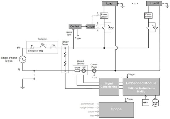
Figure 1.
Block diagram of data collecting jig. adapted from [9].
The control module senses the AC mains zero crossing; therefore, a precise timing is achieved in every power ON or OFF event. The load power control is provided by a relay in parallel to a TRIAC, each with its independent driver module. The TRIAC provides precise power switching at a giving point of the AC mains cycle while the relay operates as a conventional switch. As the relay presents a delay between the relay driver signal and the actual opening/closing of the relay contacts, a power sensor provides a precise indication of when a load is actually powered. It is possible to trigger a load only with the relay or the TRIAC, as well as with both simultaneously. Triggering only the TRIAC makes it possible to obtain a dimmer effect on the load(s).
The signal conditioning module has low pass filters and differential amplifiers so that the sensors’ signals are adequate to the embedded module analog to digital converter. The embedded module uses a National Instruments MyRio [39] board with the following functionalities: A/D conversion, load event registering obtained by the trigger signal sent by the control module, and dataset storage in a non-volatile storage device (such as a USB flash disk).
Figure 2 shows the synthetic LIT-Dataset Jig. An aluminum structure and an acrylic panel were used to support the jig’s components. The wiring is inside PVC ducts. On the left are the power connection, auxiliary power supplies, and the sockets for the jig’s equipment power supplies. The protection board is on the left side. The eight sockets for the monitored loads are on the top right, and below are the relays and TRIACs, and the control and driver boards. In the center of the board are the voltage and current sensors. On the bottom right are the conditioning boards and the MyRio Embedded Module.
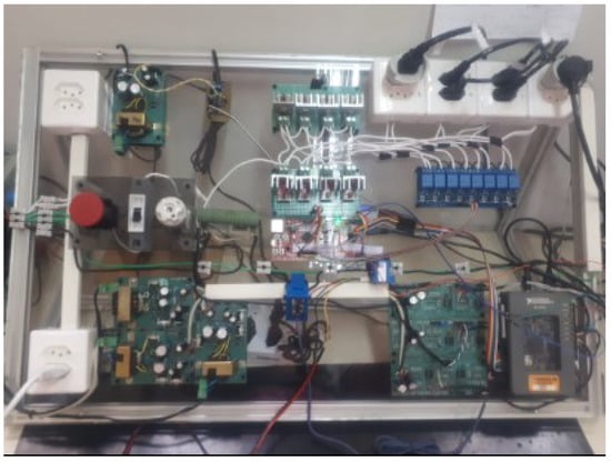
Figure 2.
Data collecting jig.
4.1.2. Data Collecting Jig Software Architecture
The embedded module block diagram is presented in Figure 3. The signal conditioning board delivers the conditioned signals from the voltage and current sensors to the MyRio module. The MyRio FPGA implements an acquisition loop that operates at 15,360 Hz, as per DSReq 6 s. On every cycle of this loop, a set of three 12-bit samples is obtained, corresponding to the A/D conversions. A GPS receiver sends a Pulse Per Second (PPS) signal, which is grouped in a data tuple with the sample signals, indicating precise 1 s periods, typically less than 100 ns jitter. An 8-bit ID and an event notification signal are also grouped in this data tuple to indicate the samples when the control module commands a load event.
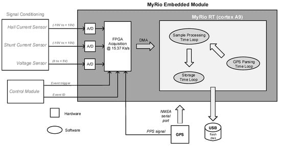
Figure 3.
Block diagram of data acquisition using the MyRio device. Adapted from [9].
The real-time application runs into the CORTEX A9 processor, composed of three NI LabView timed loops, which act as independent periodic threads. The tuple is sent by the FPGA to the real-time application via DMA. An external GPS receiver sends the NMEA strings to the GPS Parsing Timed Loop. The absolute time fields are decoded from a specific NMEA message (GPRMC) and converted to a 32-bit time-stamp value. The Sample Processing Timed Loop uses this 32-bit time-stamp, together with the event information contained in the tuple received from the FPGA, to store the time-stamped events into the event annotation file. This loop also shifts each 12-bit sample of the tuple one bit to the left and adds the PPS signal as its least significant bit, thus, allowing a precise identification of the samples during which the 1 s transitions occurred. The resulting 13-bit sample data is sent to the Storage Timed Loop via an internal FIFO, which stores the data for each of the sample inputs as a separate field of a NI Technical Data Management Streaming (TDMS) file into the USB flash disk attached to the MyRIO. The TDMS file may be processed by a PC application, to add its collected data to the LIT-Dataset.
4.1.3. Collected Data
For the synthetic subset, 26 different load configurations, divided into 16 load classes (Table 5), were used, as well as their combinations (2, 3, and 8 loads). “Load configurations” means that one load may have more than one power level and/or that more than one equipment of the same class was used (e.g., two appliances of class LED lamp).
Table 5.
Characteristics of the synthetic subset of the LIT-dataset.
Linear and non-linear loads, ranging in power from 4 W up to 1.5 kW. The loads are powered on at different angles of the mains cycle, as per Table 6. Different turn-on trigger angles affect the loads inrush current, resulting in distinct waveform acquired at each angle. Each acquisition is commanded by the control board and consists of 16 voltage/current waveforms at the specified angles. The number of individual and multiple-loads acquisitions are presented in Table 7, in a total of 104 acquisitions, corresponding to 1664 waveforms. The number of acquisitions for multiple loads were limited by the jig’s maximum power (1 kW).
Table 6.
Turn-on trigger angles.
Table 7.
Loads combination.
The sequence of events (ON and OFF) for the single and multiple loads are presented in Figure 4.
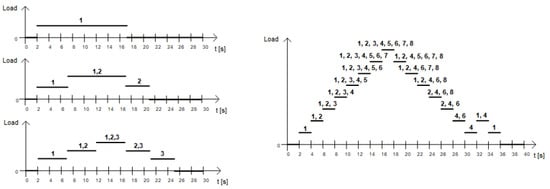
Figure 4.
Data collecting jig: single, two, three, and eight loads ON and OFF events.
4.1.4. Accuracy of the Jig
The jig’s hardware initially went through a calibration process, and then its accuracy was evaluated based on a comparison with laboratory-grade measurement equipment.
The calibration process consisted of collecting data from resistive loads that were measured with an HP bench multimeter with a 5-digit-resolution and a precision better than 0.1 %. Since the voltage and current waveforms are bipolar (positive and negative values) but the 12-bit measurements of the A/D converters from the MyRio are unipolar (0 to 4095), an offset value corresponding to inputs at zero must be determined; as well as the gain factor to convert a binary value produced by the ADC to a voltage or current value (in Volts or Amperes). This calibration process is performed before every acquisition on the Jig, and the calibration values (Ki, Kv, ZeroOffsetI, ZeroOffsetV) are reported in the file config_processed available in every acquisition folder of the LIT-Dataset.
The determination of the jig’s accuracy was performed by connecting an oscilloscope (Agilent Infiniium 54830D) and a current probe (Tektronix A6302) during the acquisitions. A total of 28 acquisitions with different loads were performed while data were simultaneously acquired by the Jig and by the scope. Data from both sources were stored as spreadsheets and imported into MATLAB for comparison. Over the 28 acquired voltage and current waveforms, the maximum error was 3.2 % with a mean value of 2.1 %. This value of accuracy was considered as acceptable for a NILM dataset. Most datasets do not provide an accuracy evaluation for comparison.
4.2. Simulated Subset
The simulated subset consists of data collected from twenty-eight different simulated loads grouped into seven kinds of electrical models, each one containing up to four power variations. The loads, waveform generation, and simulated subset settings are detailed as follows.
4.2.1. Loads
In this subset of LIT-Dataset, the electrical circuits are: (a) resistor; (b) resistor and inductor; (c) diode rectifier with a resistor; (d) diode full-wave bridge rectifier with resistor and capacitor; (e) thyristor rectifier with resistor; (f) thyristor rectifier with resistor and inductor; and (g) universal motor. The load templates were chosen according to the load profile of electrical appliances commonly found in consumer units [40], such as drill (universal motor), mobile phone charger (different types of rectifiers), fan (universal motor), hairdryer (universal motor), LED lamp (different types of rectifiers), incandescent lamp (resistor), router (different types of rectifiers), and vacuum cleaner (simplified by resistor and inductor).
The diagram of the simulated subset is shown in Figure 5, in which each block represents a different load. The switching control of each load is automated, and the trigger time can be previously adjusted.
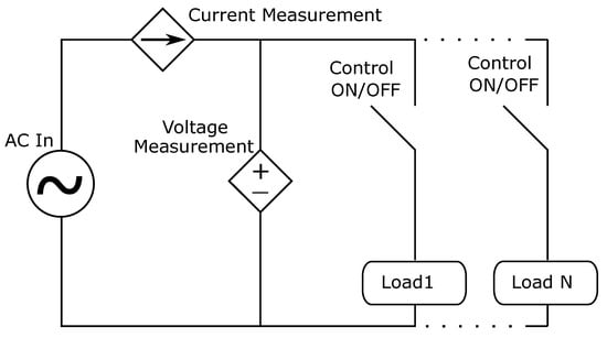
Figure 5.
General diagram of the simulated subset.
To implement each set of loads with different electrical power from circuits (a)–(f), the Power Eletronics Library from Matlab/Simulink was used, as shown in Figure 6: (a) resistor, (b) resistor and inductor, (c) diode rectifier with resistor, (d) diode bridge with resistor and capacitor, (e) thyristor rectifier with resistor, (f) thyristor rectifier with resistor and inductor.
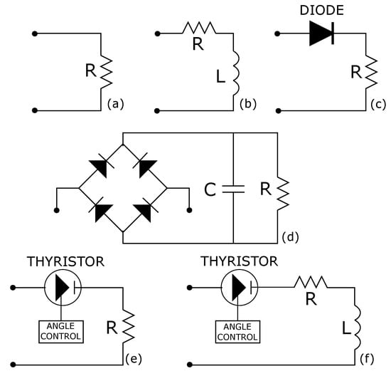
Figure 6.
Diagrams of simulated loads, being (a) resistor, (b) resistor and inductor, (c) diode rectifier with resistor, (d) diode bridge with resistor and capacitor, (e) thyristor rectifier with resistor, (f) thyristor rectifier with resistor and inductor.
For the implementation of the universal motor (g), a mathematical model based on [41] was used. Figure 7 shows the diagram that represents this model, in which the following parameters are included: rated power, rated terminal voltage, rated speed, armature winding inductance (), series field winding inductance (), rated frequency of supply voltage, armature winding resistance (), series field winding resistance (), rotor inertia (J), speed at which magnetization curve data was taken (). To connect the math model with other circuits, the generated signal was connected to a current source generator and sent to other blocks, i.e., electrical—mathematical interface in MATLAB-Simulink.
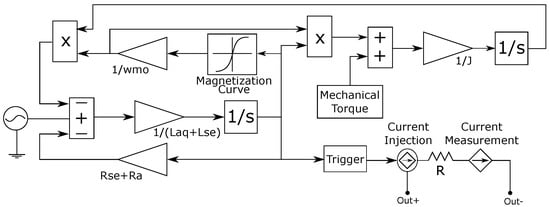
Figure 7.
MATLAB-Simulink block diagram of Universal Motor Model.
4.2.2. Waveform Generation
To automate the waveform generation, an automatic parameter variation method was implemented. With that method, it is possible to vary: up to seven different load combinations for each waveform; up to four different values of the electrical components for each circuit; the total time of the simulation; the load combination; and the trigger time of the circuits, with three different options of switching (turn-ON and turn-OFF) angles: 0, 45, and 90 degrees. The four parameters variations, resulting in four different rated power levels for each set of loads, are detailed in Table 8, where: (a) resistor; (b) resistor and inductor; (c) diode rectifier with a resistor; (d) diode full-wave bridge rectifier with resistor and capacitor; (e) thyristor rectifier with resistor; (f) thyristor rectifier with resistor and inductor; (g) universal motor.
Table 8.
Load parameters.
4.2.3. Configuration of Simulation Scenarios
To create different simulation scenarios, six configuration settings can be used, as follows: ideal (DB-1); with stray inductance, representing the equivalent of the electrical network (DB-2); with stray inductance and harmonics (DB-3); and with stray inductance, harmonics, and additive white gaussian noise (AWGN), with 60 dB, 30 dB, and 10 dB of SNR (DB-4, DB-5, and DB-6), as shown in Table 9. Each of the six configurations are applied to all the loads, resulting in 4824 waveforms, being 804 for each configuration. Therefore, it is possible to evaluate the impact of harmonics and noise (with different intensities) and to compare to an ideal scenario, to the performance of detection, feature extraction, and classification methods. This type of analysis can support the proposal of more robust and applicable methods in different NILM scenarios.
Table 9.
Simulated subset settings.
The first scenario (DB-1), was an ideal setting, without stray inductance and harmonic content in the voltage waveform. The second one (DB-2), include stray inductance. The characteristics of the electrical network in our laboratory were used to select the values of the inductor and resistor, resulting in L = 1 µH and R = 2 m. The third scenario (DB-3), includes stray inductance and a voltage source with harmonics, based on the voltage acquisition in our laboratory. The last three include a voltage source with harmonics, stray inductance, and different levels of AWGN.
4.3. Natural Subset
The Natural subset of the LIT-Dataset consists of recording where a natural load shaping occurs, in the sense that waveforms are registered in a real-world environment (residential, research lab, commercial, industrial) over longer periods of time. To precisely detect and record the load events, sensors that detect power-ON, power-OFF, and power-level-changes are attached to each load, therefore, while the aggregated current and voltage are recorded, so are the individual load events.
4.3.1. Natural Subset—Data Collection Architecture and Implementation
Accurate time synchronization is an important requirement in this scenario, in which time-stamped data should be provided by distributed nodes and then correlated with a limited jitter among them. Concerning specifically the development of the Natural subset of the LIT-Dataset, an infrastructure composed of a centralized acquisition device and a large number (50+ units) of networked wireless sensors is required. These nodes are attached to each load to detect load events, such as ON-OFF transient, change of state and power variations, and send the event data to the centralized acquisition element so that they can be later consolidated and correlated with the acquired voltage and current data.
This infrastructure, from this point on referred to as Natural Subset Acquisition System (NSAS), depends on time synchronization with accuracy and precision of at least 1 ms, to facilitate the correlation between the events obtained by the distributed event detection modules and the voltage and current samples obtained by the centralized acquisition element. Additionally, considering the large number of modules to be installed and their distributed characteristic, they are required to be built with low-cost components. In this sense, even though there are several techniques and protocols that address the precise time synchronization issue, most of them rely on specialized hardware and/or software solutions, thus incurring a relatively high cost to deploy the synchronization network [42,43].
An overview of the architecture used to collect a dataset of traces with natural load shaping is presented in Figure 8. It is important to notice that the voltage and current traces for the aggregate of the loads are collected at a single point, namely at the sensors next to the fuse box. The distributed nodes only detect power events (ON, OFF, and power changes) and record the occurrence of such events locally. It is this recording that requires a millisecond timing accuracy, achieved through the synchronization mechanism implemented by the NSAS.
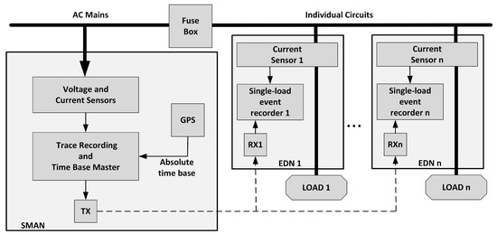
Figure 8.
Overview of the architecture for collecting a natural load shaping subset.
The principle of operation of this low-cost synchronization network is to have a time base master, with a GPS based real-time clock, to periodically broadcast a two-byte synchronization packet to all nodes in the synchronization network.
To avoid delays imposed by complex packet-based protocols, an approach that implements the synchronization task right before the PHY is used. This is performed using a low-cost, byte-based RF 433 MHz transmitter-receiver pair [44], similar to the one used in [45] for an application with similar requirements. The typical reception delay for this solution is about 300 µs, which meets NSAS timing requirements of 1 ms.
Furthermore, the main contribution of this proposed architecture is its low cost (about one dollar for the receiver), in a way that its impact on the cost of the whole NSAS is minimized. The block diagram of the Natural Subset Acquisition System is presented in Figure 9.
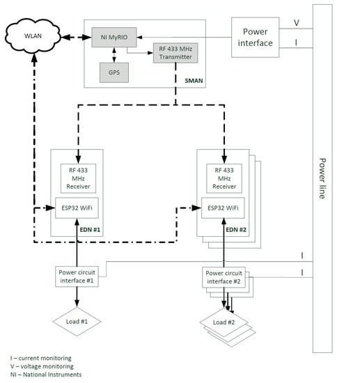
Figure 9.
Block diagram of the Natural Subset Acquisition System (NSAS).
The Synchronization Master and Acquisition Node (SMAN), on the top of the block diagram, is implemented by using a National Instruments MyRIO module [39] attached to a GPS module and the 433 MHz RF transmitter [44]. The MyRIO module is connected to the other NSAS modules via a WLAN and is programmed, via LabView, to perform the SMAN main tasks. The RF transmitter receives a digital timing synchronization signal as input and broadcasts it in the 433 MHz band at a rate of up to 2400 bps. The EDNs (Event Detection Nodes) consist of ESP32 Heltec WiFi modules, as well as 433 MHz RF receivers. The ESP32 Heltec kit is a low-cost development board, which is programmable using the Arduino IDE and corresponding libraries to perform the EDN tasks. It connects to the other NSAS modules via a WiFi-based WLAN. The RF receivers are responsible for receiving the signal that is broadcast by the RF transmitter of the SMAN. Each EDN is physically connected to a Power circuit connection element (interrupter, outlet, etc.), so it can perform the sampling of current to detect variations that indicate a load switch event (ON, OFF, or other state change such as changing from standby to active mode).
The SMAN is responsible for acquiring the voltage and current samples at a frequency of 15,384 Hz, which is slightly above the minimum 15,360 Hz frequency specified for the LIT-Dataset due to the MyRio-timer configuration options. The SMAN is also responsible for collecting and storing the event data sent by the EDNs via the WLAN. The GPS module provides the SMAN with an absolute time reference on every second employing the PPS (pulse per second) signal, whose typical jitter is of hundreds of nanoseconds. This time reference is used to ensure that the millisecond data used by the SMAN to synchronize the EDNs is synchronized to an absolute reference, regardless of potential clock drifts presented by the SMAN itself (typically 10 ppm).
Upon detection of an event on a load connected to a monitored power circuit connection element, the corresponding EDN sends the event data to the SMAN via the WLAN and waits for the event acknowledgment. If the acknowledgment times out, the event is sent again. The EDNs also communicate with the SMAN by means of “abs time req” messages, which are sent during EDN initialization. The SMAN responds with an “abs time resp” message containing the absolute time and date, with a resolution of one second, obtained from the GPS receiver. This transaction is responsible for performing a relatively coarse synchronization (i.e., with an accuracy of one second) between the SMAN and the EDNs. The synchronization between EDNs and SMAN is improved to millisecond-accuracy upon reception of an RF message, broadcast by the SMAN, which consists of a 16-bit synchronization code. The SMAN sends the code at a rate of 1000 bps (i.e., one bit per millisecond) on every second boundary (1 Hz). Hence, upon completion of the reception and validation of the code, every EDN shall (re)adjust the millisecond’s field of its current time to 16, corresponding to the 16 ms that have passed from the latest second boundary to the end of reception of the last bit of the synchronization code.
As the typical clock drift for the EDN hardware is 10 ppm, a drift of 0.5 ms would occur every 50 s; therefore the resynchronization rate of 1 Hz is, theoretically, widely sufficient to ensure that the EDNs remain synchronized with the SMAN even if 98% (49 of 50) of the RF synch messages are lost. Additionally, the typical jitter of the RF link (300 µs) is small enough not to introduce indeterminism on the millisecond value to be adjusted into the EDNs.
However, it is observed that some EDNs present much higher drift rates than the typical case; in some cases, more than 1000 ppm have been observed under operating conditions, which would compromise the millisecond precision required by the system. Therefore, it is necessary to implement an extra strategy to prevent desynchronization between the several EDNs and the SMAN that compose the NSAS.
The drift correction strategy consists of the algorithm shown in Figure 10a. Initially, the timer tick is set to 1000 µs (1 ms), which is the default period for time-stamp updates. Upon reception of a synch word (i.e., on every second), the EDN compares the millisecond on which the synch word has been effectively received with the millisecond on which it should have been completely received (16, because of the 16-bit synch word sent at 1000 bps starting from 0 ms at the SMAN) (line 6). The more positive the difference between the former and the latter, the more this EDN´s specific tick is being advanced in relation to the nominal tick frequency (1 kHz) because of its clock drift; the same happens when the difference is negative, meaning that the clock drift is causing the EDN tick to be delayed. Next, the EDN timer period is proportionally adjusted (lines 9 and 10), so the next ticks can compensate the clock drift by an increase (or decrease) of the programmed tick frequency.
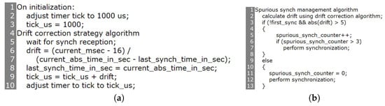
Figure 10.
Algorithms used in Event Detection Nodes (EDNs). (a) Drift correction algorithm. (b) Spurious synch management algorithm.
Another algorithm, shown in Figure 10b, is implemented to take into account possible spurious synchronization words that can be received due to noise at the RF link. This is a real concern, as the 433 MHz radios used for the NSAS are very susceptible to such noise, and the implemented synchronization algorithm, which is supposed to be simple and deterministic, does not make use of any software checking mechanisms to improve data reception reliability.
The spurious sync management algorithm analyzes the calculated drift obtained from the algorithm of Figure 10a. If this is the first synchronization, the calculated drift is probably correct, as there is no previous synchronization between the SMAN and this EDN. If this is not the first synchronization, and the absolute calculated drift value is greater than a specified limit of 5, corresponding to 5000 ppm. Since 5000 ppm is significantly larger than the typical 10 ppm drift, or even the 1000 ppm drift occasionally detected, a spurious sync word has likely been received on a random time, leading to a drift miscalculation; in this case, the EDN ignores the spurious sync unless it has already been received more than three times in sequence (as tested in line 6). If that happens, the first received sync was probably spurious, and thus, the new sync is assumed to be the correct one.
4.3.2. Natural Subset—Collected Data
For the natural subset, 14 different load configurations, divided into 11 load classes (Table 10), were used, as well as their combinations. The 3-load combination has 30 s of duration and 6 events. The 7-load combinations have 2 h of duration and 20 events or more. The load configurations mean either that one load has more than one state or that more than one device of the same class was used.
Table 10.
Characteristics of the natural subset of the LIT-dataset.
4.4. LIT-Dataset Integration to NILMTK
As NILMTK uses an internal data format (NILMTK-DF), a data format conversion function must be implemented such as those already available for REDD, Smart, and UK-Dale [36]. Such a function was implemented for the LIT-Dataset; hence, its waveforms can be processed in NILMTK. Figure 11a,b presents one of the LIT-Dataset waveforms, an incandescent light bulb that is also presented in Section 5.
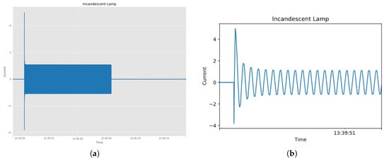
Figure 11.
A LIT-Dataset waveform of an incandescent lamp presented in NILMTK. (a) Complete waveform. (b) Image zoomed into power-ON event.
5. Results and Analysis
The results of data collection for each subset and the corresponding analysis are detailed as follows.
5.1. Synthetic Subset
The original aspects of the Synthetic subset include multiple concurrent loads of distinct classes, with precise turn-ON and turn-OFF control and annotations of these events with an accuracy better than 5 ms. These annotations (labels) can later be used to validate event detection, transient feature extraction, and load classification methods.
The synthetic subset is composed of 1664 acquisition for single, double, threefold, and eight-fold concurrent loads. For every load or load combinations, acquisitions are made for 16 distinct turn-on trigger angles.
In Figure 12a, the acquisition of an incandescent lamp with a turn-on trigger angle of 90 degrees is shown, while Figure 12b,c present a detailed (zoomed-in) view of the turn-ON and turn-OFF events, respectively. The high inrush current is due to the variation of the filament resistance of the lamp, as its temperature rises. The inrush current is also dependent on the turn-on trigger angle. This unique transient response may be beneficial to the detection as well as the classification methods. In these figures, the up-arrow indicates a turn-ON event while the down-arrow indicates a turn-OFF event.
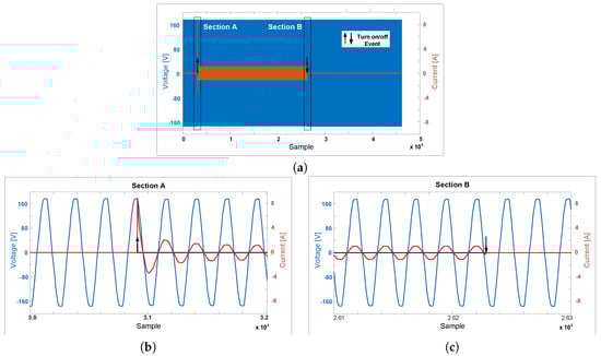
Figure 12.
Jig acquisition of a single load: incandescent lamp—trigger angle of 90 degrees. (a) Complete acquisition—AC mains voltage and current. (b) Turn-ON event. (c) Turn-OFF event.
A single load acquisition of a laptop power supply is presented in Figure 13a, for a turn-on trigger angle of 45 degrees. A detail of the turn-ON and turn-OFF events are presented in Figure 13b,c. Typically a power supply first stage consists of a diode rectifier followed by a capacitor. The inrush current depends on the capacitance and the turn-on trigger angle and is very high compared to the steady-state peak current. This transient response is very rich in detecting an event and classify the load. The steady-state low power may be challenging to detect and classification steady-state based methods.
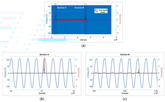
Figure 13.
Jig acquisition of a single load: laptop power supply—trigger angle of 45 degrees. (a) Complete acquisition—AC mains voltage and current. (b) Turn-ON event. (c) Turn-OFF event.
An example of a double load acquisition is presented in Figure 14. An oil heater (520 W) is turned-on (trigger angle of 135 degrees), and then a LED lamp (6 W) is turned on, also at trigger angle of 135 degrees. Later, the heater is turned off, and finally, the lamp is turned off. This is an interesting combination of linear and non-linear loads of significantly different power levels. Details of the turn-ON and turn-OFF events are presented in Figure 15a–d. As the oil heater has a higher power, the turn-ON event of the LED lamp may be challenging to detect, as Figure 15b shows, likewise, the turn-OFF event of the LED lamp, as shows Figure 15d.
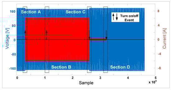
Figure 14.
Jig acquisition of two loads: oil heater and LED lamp—trigger angle of 135 degrees.
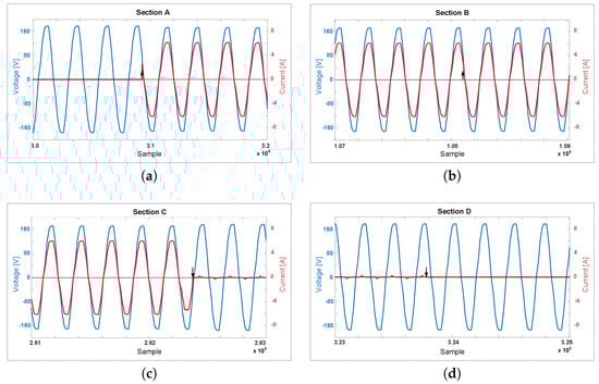
Figure 15.
Jig acquisition of two loads: oil heater and LED lamp—trigger angle of 135 degrees. (a) Turn-ON event section A: heater turned on. (b) Turn-ON event section B: LED lamp turned on. (c) Turn-OFF event section C: heater turned off. (d) Turn-OFF event section D: LED lamp turned off.
A three loads combination composed of a hairdryer, a LED lamp, and a drill is presented in Figure 16, with a turn-on trigger angle of 225 degrees. The hairdryer, at the low power level setting, has a half-wave diode rectifier, hence, an asymmetrical load. The drill high inrush current may also be observed.
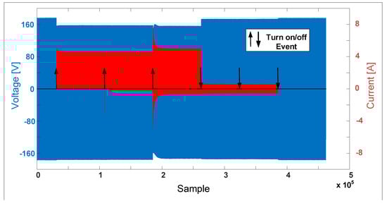
Figure 16.
Jig acquisition of three loads: hairdryer at low power level, LED lamp, and drill—trigger angle of 225 degrees. AC mains voltage and current.
Finally, Figure 17 shows an example of eight loads combination: a LED lamp, a laptop power supply, a microwave, a cell phone charger, a soldering station, an incandescent lamp, an oil heater, and a smoke extractor with turn-on events triggered at 270 degrees. The combination of eight loads with different power levels, linear and non-linear characteristics, is important to evaluate detection and classification methods.
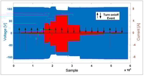
Figure 17.
Jig acquisition of eight loads: LED lamp, laptop power supply, microwave, cell phone charger, soldering station, incandescent lamp, oil heater, smoke extractor—trigger angle of 270 degrees. AC mains voltage and current.
5.2. Simulated Subset
The circuits with (a) resistor; (b) resistor and inductor: (c) diode rectifier with resistor; (d) diode full-wave bridge rectifier with resistor and capacitor; (e) thyristor rectifier with resistor; and (f) thyristor rectifier with resistor and inductor were evaluated with a test bench. The load current and mains voltage were acquired using voltage and current probes and an oscilloscope, with the simulated loads configured as presented in Table 11.
Table 11.
Parameters of real components in the test bench.
In addition to the voltage and current measurements using the test bench, the amplitude and phase of each harmonic of the waveform of the voltage of the power network was measured. These values, presented in Table 12, were included in the voltage source block in the simulator and used in all simulations that included harmonic contents (configurations DB-3 to DB-6 in Table 9). The amplitude is presented with respect to the fundamental component: 60 Hz and peak voltage of 179 V).
Table 12.
Measurement of voltage and phase of harmonics in the power network.
The parameters presented in Table 11 and Table 12 were used in the simulation framework developed in Matlab/Simulink. Then, the measured and the simulated waveforms were compared, as exemplified in Figure 18.
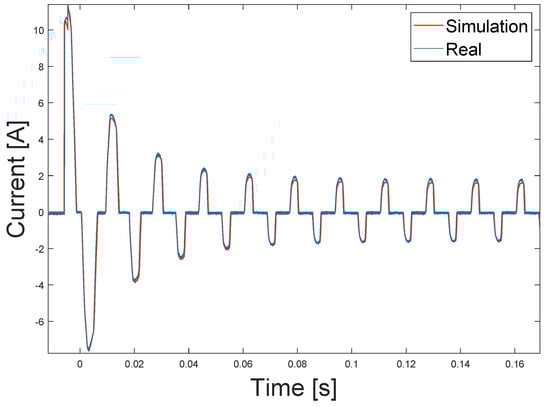
Figure 18.
Measured and simulated current of the full-wave bridge rectifier load. Adapted from [10].
One way to validate the simulation is by comparing the waveform’s electrical parameters, such as transient and steady-state current and voltage peaks, power factor (PF), and mean squared error (MSE) of the samples of the measured and simulated waveforms, as suggested in [46]. Therefore, Table 13 and Table 14 present such comparisons for the simulations proposed in this work. The results presented in these tables validate the presented simulation approach for circuits (a) to (f).
Table 13.
Validation parameters (absolute current and voltage peak differences).
Table 14.
Validation parameters (power factor (PF) and mean squared error (MSE)).
Finally, the validation of the last circuit (g), the universal motor, was performed using an electric drill of as a reference, with two-speed selection. The procedure was conducted in two stages. Firstly, the current and voltage signals of the electric drill were acquired in different scenarios, i.e., switching angle and load conditions. Then, the acquired signals were used to obtain the field and rotor resistances and inductances of the model presented in Figure 6. The final obtained values used in this model were:
- Rated power = 325 W;
- Rated terminal voltage = 120 Vrms;
- Rated speed = 2800 rev/min;
- Armature winding inductance, = 10 mH;
- Series field winding inductance, = 26 mH;
- Rated frequency of supply voltage = 60 Hz;
- Armature winding resistance, = 0.6 ;
- Series field winding resistance, = 0.1 ;
- Rotor inertia, J = 0.0015 kg · m;
- Speed at which mag. curve data was taken , with rev/min.
Secondly, with these parameters, the comparison of the real and simulated current of a universal motor is presented in Figure 19. As can be observed, the waveforms present similar values in transient and steady-state. The MSE between these waveforms is .
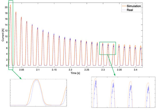
Figure 19.
Comparison of the measured and simulated waveforms of a drill. Adapted from [10].
Concerning the generation of the waveforms that compose the Simulated subset, Figure 20 presents an example of the current waveform generated in the proposed subset (DB-5), in a double load scenario where the first load is a resistor and inductor circuit (section A, Figure 21a and section C, Figure 21c) and the second load is the universal motor (section B, Figure 21b and section D, Figure 21d).
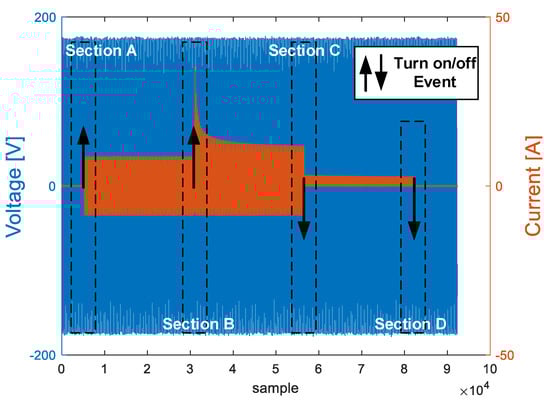
Figure 20.
Simulated subset complete acquisition: RL and universal motor. AC mains voltage and current.
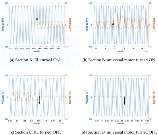
Figure 21.
Sections (a–d): RL and universal motor.
The sampling frequency for the Simulated subset is also 15,360 Hz and switching instants (ON or OFF) are precisely controlled at the sample level. For each switching-event, the load is also properly labeled, allowing the correct use of supervised classifiers and transient feature extraction methods.
The simulator’s functionality allows for the generation of single-load waveforms as well as the combination of two, three, four, five, six, and seven loads. Such combinations can be accomplished using a MATLAB script that automates the waveform generation, using pre-defined trigger instants and types of loads that are selected in each simulation (The MATLAB-Simulink template to generate this dataset is made publicly available at https://github.com/hellenancelmo/Simulated-LIT-dataset). Hence, this subset can be extended to other types of residential, commercial, and low-voltage industrial loads.
5.3. Natural Subset
To illustrate the validation of the data collection system of the Natural subset (NSAS—Figure 9) a 3-load combination recording is presented. In this case, the EDNs are identified by a code transmitted in the data package to the Synchronization Master and Acquisition Node (SMAN). Table 15 presents the three loads used, the number of the respective EDN, and the corresponding identification code for power-ON and power-OFF events.
Table 15.
Natural subset Devices (Acquisition Example).
The following sequence of load switching occurred: (i) turn-ON incandescent lamp; (ii) turn-OFF incandescent lamp; (iii) turn-ON LED lamp; (iv) turn-OFF LED lamp; (v) turn-ON drill; (vi) turn-OFF drill, generating the voltage and current curves represented in Figure 22a.
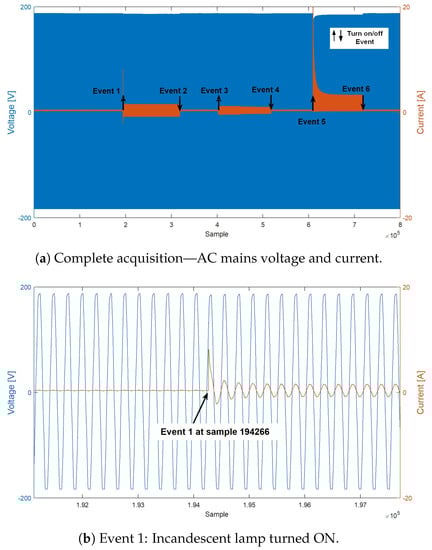
Figure 22.
Natural subset: incandescent lamp, LED lamp, and drill.
Table 16 presents all six events. The actual instant of the power-ON/power-OFF events can be obtained by analyzing the waveforms, as represented in Figure 22b, where the turn-ON Event 1 at sample 194,266 is shown. These values are presented in column “Event observed in waveform (in samples)” and represent the ground truth. The EDN data packet contains the time stamp and event code in the format . From the data packet, the reported time of the event (in samples) is obtained using the time-stamp of the first sample in the waveform. The corresponding error, measured in the number of samples, corresponds to the distance (in samples) between ground-truth and the detected event. The sampling frequency is 15,360 Hz; hence, each sample corresponds to 65.1 µs.
Table 16.
Events representations file.
5.4. Analysis of the Results
In this section, the analysis of the three subsets is presented. Table 17 illustrates the high-frequency datasets (initially presented in Section 2.2, Table 3), now including the three LIT-Dataset subsets.
Table 17.
Comparison of high-frequency NILM datasets.
From the results presented previously in this section and by the comparative analysis summarized in Table 17, the distinct features of the LIT-Dataset are:
- It consists of three subsets, each one with multiple concurrent loads of distinct types, including those found in residential, commercial, and low-voltage industrial environments.
- The Synthetic subset contains waveforms that were collected on a jig, with precise control of turn-ON and turn-OFF of up to eight loads (thus, synthetic load shaping).
- The Simulated subset contains waveforms that were collected by simulation; hence, the simulated circuits can be easily modified to match several distinct real-world scenarios.
- The Natural subset contains waveforms that were collected in a real-world environment; hence, representing what a NILM system would actually monitor and analyze.
- Ground Truth, an essential requirement for the evaluation of NILM algorithms and techniques, is achieved by labeling, at sample level, the load events, i.e., when each load has a change in power, due to power-ON, power-OFF of power-level-change. For each load event, the corresponding load and event type is recorded in the label.
- The resolution of the load event labeling is better than 5 ms; hence, identifying the mains semi-cycle where the load event occurs.
5.5. Considerations on the Design Process
The LIT-Dataset, composed of three subsets, is the result of a design process that started with Requirements Engineering, including requirements harvesting of the Stakeholders Requirements, identification of the source and derived requirements, data format design, development process of the Enabling Systems (Jig, Simulator, and network of NSAS), validation of the enabling systems, data collection, data validation, and publication of the dataset files and user support documentation.
Following such a well-defined design process was beneficial to keep the project on track and according to established project planning. Even so, as with most engineering projects, some difficulties presented themselves during the process. The most relevant and time-consuming were:
- Due to cost restrictions of each NSAS module, an ESP32 processor was selected that we had no previous experience on. It turned out that the particular model selected had a design fault that causes the interference of the WiFi and ADCs. Some extra effort on the project was required until this problem was identified and solved (by disabling the WiFi and reconfiguration of the ADC before every A/D conversion).
- The low-cost transmitter-receiver 433 MHz RF synchronization network resulted in a relatively high packet loss rate. Again, an extra effort was required to identify the problem and design an algorithm to cope with such high packet losses.
- Certainly, the most unexpected difficulty was to finish the project, on-time, during the COVID-19 Pandemic. Significant changes in the work environment, basically moving all activities to home office, required an unexpected amount of extra work.
As the initial planning included very little slack time to cope with such difficulties, the solution to keep the original schedule of the project was to increase the weekly work effort of the participants. The collection of data for the Natural subset is somewhat delayed. The aim is to continue data collection for all subsets.
6. Conclusions
The LIT-Dataset was presented chronologically. Its rationale in supporting our own NILM development as well as making it publicly available. Its conception; its requirements elicitation and specification, based on an evaluation of available NILM datasets and the additional needs. Its design, structuring the LIT-Dataset into three subsets, each exploring a different load-set context. The design and implementation of the supporting systems for each of the subsets: jig, simulator, and NSAS. Its evaluation and validation, based on the comparison of simulated loads to real-world loads as well as its usage in NILM techniques. Finally, its publication (the LIT-Dataset is publicly available, upon free registration, at http://dainf.ct.utfpr.edu.br/~douglas/LIT_Dataset), with detailed documentation and usage scripts.
The three subsets consider the scenarios of (1) a set of up to eight loads that are controlled (on and off switching) individually during the recording of aggregated current and load events; (2) a set of simulated loads that are recorded under conditions that would be difficult in real-world situations, either because they are uncommon or due to hazardous scenarios such as short-circuits; and (3) a set of loads monitored during their daily use. The first subset is the named Synthetic load shaping, as the “on” and “off” events are controlled, the second is named Simulated, and the third is named Natural load shaping as there is no influence on the loads during the recording period.
Among the distinct features of the LIT-Dataset, as described in Section 5.4, is the labeling of the load events at sample level resolution and with an accuracy better than 5 ms; the availability of such precise timing information that also includes the identification of the load and of the sort of power event is an essential requirement both for the evaluation of NILM algorithms and techniques, as well as, for training of NILM systems, particularly those based on Machine Learning.
Our contribution is to make publicly available a new dataset whose combination of features makes it unique. These features are: (1) the availability of load-event labels, with an accuracy better than 5 ms, providing ground-truth information of the load events, (2) the availability of three subsets (as described above), (3) recording scenarios with up to eight concurrent loads, (4) combination of residential, commercial and low-voltage industrial loads, and (5) load shaping scenarios with low-power loads being switched when high-power loads are energized.
To summarize the benefits of these contributions, concerning the availability of load-event labels, the LIT-Dataset achieved the best accuracy among the datasets that were analyzed (Table 17). This is an important characteristic for those using a dataset to validate event detection and load classification algorithms. Having loads recorded individually and concurrently also provides the required information for training as well as for evaluating the performance of NILM algorithms. Furthermore, scenarios where low-power loads switching when higher-power loads are powered-on, provides challenging test cases for these NILM algorithms.
The LIT-Dataset was presented here, from its conception to implementation, analysis of results, and publication. However, data collection is in progress as new loads, and new scenarios are frequently recorded and added to the dataset.
Author Contributions
Conceptualization, D.P.B.R., F.P., H.C.A., and C.R.E.L.; data curation, D.P.B.R., F.P., H.C.A., R.R.L., L.d.S.N., L.T.L., B.M.M., and J.R.L.d.S.; formal analysis, D.P.B.R., A.E.L., R.R.L., and E.O.; funding acquisition, D.P.B.R., A.E.L., J.S.O., and R.B.d.S.; investigation, D.P.B.R., F.P., H.C.A., A.E.L., E.O., and L.d.S.N.; methodology, D.P.B.R., F.P., H.C.A., A.E.L., C.R.E.L., and R.R.L.; project administration, D.P.B.R., J.S.O., and R.B.d.S.; resources, D.P.B.R., C.R.E.L., and R.R.L.; software, D.P.B.R., H.C.A., C.R.E.L., R.R.L., L.T.L., and B.M.M.; supervision, D.P.B.R., J.S.O., and R.B.d.S.; validation, D.P.B.R., F.P., H.C.A., A.E.L., C.R.E.L., E.O., L.d.S.N., and L.T.L.; visualization, D.P.B.R., L.d.S.N., and J.R.L.d.S.; writing—original draft preparation, D.P.B.R., F.P., H.C.A., A.E.L., C.R.E.L., R.R.L., and E.O.; writing—review and editing, D.P.B.R., F.P., and E.O. All authors have read and agreed to the published version of the manuscript.
Funding
This study was fully financed by Agência Nacional de Energia Elétrica (ANEEL) and Companhia Paranaense de Energia Elétrica (COPEL) under the research and development program (project PD2866-0464/2017).
Acknowledgments
The authors would like to thank COPEL and ANEEL for the support and promotion in the research project PD2866-0464/2017.
Conflicts of Interest
The authors declare no conflict of interest. The funders had no role in the design of the study; in the collection, analyses, or interpretation of data; the authors affiliated to the funder company had the role of manuscript revision and evaluating the request for publication.
Abbreviations
The following abbreviations are used in this manuscript:
| AC | Alternating current | MSL | Multiple Simultaneous Loads |
| AMPds | Almanac of Minutely Power Dataset | NILM | Non-Intrusive Load Monitoring |
| ANEEL | Agência Nacional de Energia Elétrica | NILMTK | NILM Toolkit |
| API | Application Programming Interface | NMEA | National Marine Electronics Association |
| AWGN | Additive White Gaussian Noise | NoC | Number of Appliance Classes |
| BLUED | Building-Level fUlly-labeled dataset for Electricity Disaggregation | NoA | Number of Appliances |
| BLOND | Building-Level Office enviroNment Dataset | NSAS | Natural Subset Acquisition System |
| Com | Commercial | PC | Personal Computer |
| COOLL | Controlled On/Off Loads Library | PF | Power Factor |
| COPEL | Companhia Paranaense de Energia | PIR | Passive InfraRed |
| DB | Database | PLAID | Plug Load Appliance Identification Dataset |
| DCD | Data Collection Duration | PPS | Pulse Per Second |
| DF | Data Format | PVC | Polyvinyl Chloride |
| DMA | Direct Memory Access | RAE | Rainforest Automation Energy |
| DSReq | Dataset Stakeholder Requirements | REDD | Reference Energy Disaggregation Dataset |
| EMI | Electromagnetic Interference | Res | Residential |
| EDN | Event Detection Node | RF | Radio Frequency |
| FIFO | First In, First Out | RFID | Radio Frequency IDentification |
| FPGA | Field-Programmable Gate Array | SNR | Signal-to-Noise Ratio |
| GPS | Global Positioning System | SMAN | Synchronization Master and Acquisition Node |
| HES | Household Electricity Survey | SusDataED | Sustainable Data for Energy Disaggregation |
| HFED | High-Frequency Energy Data | SynD | Synthetic energy Dataset |
| iAWE | Indian Dataset for Ambient Water and Energy | TDMS | Technical Data Management Streaming |
| IDE | Integrated Development Environment | TRIAC | Triode for Alternating Current |
| Ind | Industrial | USB | Universal Serial Bus |
| Lab | Laboratory | UK-DALE | United Kingdom recording Domestic Appliance-Level Electricity |
| LED | Light-Emitting Diode | UWB | Ultra Wide Band |
| LER | Load Event Resolution | WHITED | Worldwide Household and Industry Transient Energy Dataset |
| LIT | Laboratory of Innovation and Technology in Embedded Systems and Energy | WLAN | Wireless Local Area Network |
| MSE | Mean Squared Error |
References
- International Energy Agency. World Energy Outlook; OECD Publishing: Paris, France, 2019; p. 810. [Google Scholar]
- Zoha, A.; Gluhak, A.; Imran, M.A.; Rajasegarar, S. Non-intrusive Load Monitoring approaches for disaggregated energy sensing: A survey. Sensors 2012, 12, 16838–16866. [Google Scholar] [CrossRef] [PubMed]
- Lazzaretti, A.; Renaux, D.; Lima, C.; Mulinari, B.; Ancelmo, H.; Oroski, E.; Pottker, F.; Linhares, R.; Nolasco, L.; Lima, L.; et al. A Multi-Agent NILM Architecture for Event Detection and Load Classification. Energies 2020, 13, 4396. [Google Scholar] [CrossRef]
- LIT. LIT-Dataset: A Dataset of Voltage and Current Waveforms on a Variety of Single and Multiple Loads. 2019. Available online: http://dainf.ct.utfpr.edu.br/~douglas/LIT_Dataset (accessed on 15 August 2020).
- Ruano, A.; Hernandez, A.; Ureña, J.; Ruano, M.; Garcia, J. NILM techniques for intelligent home energy management and ambient assisted living: A review. Energies 2019, 12, 2203. [Google Scholar] [CrossRef]
- Renaux, D.P.B.; Lima, C.R.E.; Pottker, F.; Oroski, E.; Lazzaretti, A.E.; Linhares, R.R.; Almeida, A.R.; Coelho, A.O.; Hercules, M.C. Non-Intrusive Load Monitoring: An Architecture and its evaluation for Power Electronics loads. In Proceedings of the 2018 IEEE International Power Electronics and Application Conference and Exposition (PEAC), Shenzhen, China, 4–7 November 2018; pp. 1–6. [Google Scholar]
- Ancelmo, H.C.; Grando, F.L.; Costa, C.H.D.; Mulinari, B.M.; Oroski, E.; Lazzaretti, A.E.; Pottker, F.; Renaux, D.P.B. Automatic Power Signature Analysis using Prony’s Method and Machine Learning-Based Classifiers. In Proceedings of the 2nd European Conference on Electrical Engineering and Computer Science (EECS), Bern, Switzerland, 20–22 December 2018; pp. 65–70. [Google Scholar]
- Pottker, F.; Lazzaretti, A.E.; Renaux, D.P.B.; Linhares, R.R.; Lima, C.R.E.; Ancelmo, H.C.; Mulinari, B.M. Non-Intrusive Load Monitoring: A Multi-Agent Architecture and Results. In Proceedings of the 2nd European Conference on Electrical Engineering and Computer Science (EECS), Bern, Switzerland, 20–22 December 2018; pp. 328–334. [Google Scholar]
- Renaux, D.; Linhares, R.; Pottker, F.; Lazzaretti, A.E.; Lima, C.; Coelho Neto, A.; Campaner, M. Designinga Novel Dataset for Non-intrusive Load Monitoring. In Proceedings of the VIII Brazilian Symposium on Computing Systems Engineering (SBESC), Curitiba, Brazil, 7–10 November 2018; pp. 243–249. [Google Scholar]
- Ancelmo, H.C.; Mulinari, B.M.; Pottker, F.; Lazzaretti, A.E.; Bazzo, T.d.P.M.; Oroski, E.; Renaux, D.P.B.; Lima, C.R.E.; Linhares, R.R.; Gamba, A.R.d.A. A New Simulated Database for Classification Comparison in Power Signature Analysis. In Proceedings of the 20th International Conference on Intelligent System Application to Power Systems (ISAP), New Delhi, India, 10–14 December 2019; pp. 1–7. [Google Scholar]
- Ancelmo, H.C.; Grando, F.L.; Mulinari, B.M.; da Costa, C.H.; Lazzaretti, A.E.; Oroski, E.; Renaux, D.P.B.; Pottker, F.; Lima, C.R.E.; Linhares, R.R. A Transient and Steady-State Power Signature Feature Extraction Using Different Prony’s Methods. In Proceedings of the 20th International Conference on Intelligent System Application to Power Systems (ISAP), New Delhi, India, 10–14 December 2019; pp. 1–6. [Google Scholar]
- Mulinari, B.M.; de Campos, D.P.; da Costa, C.H.; Ancelmo, H.C.; Lazzaretti, A.E.; Oroski, E.; Lima, C.R.E.; Renaux, D.P.B.; Pottker, F.; Linhares, R.R. A New Set of Steady-State and Transient Features for Power Signature Analysis Based on V-I Trajectory. In Proceedings of the 2019 IEEE PES Innovative Smart Grid Technologies Conference—Latin America (ISGT Latin America), Gramado, Brazil, 15–18 September 2019; pp. 1–6. [Google Scholar]
- Linhares, R.R.; Lima, C.R.E.; Renaux, D.P.B.; Pottker, F.; Oroski, E.; Lazzaretti, A.E.; Mulinari, B.M.; Ancelmo, H.C.; Gamba, A.; Bernardi, L.A.; et al. One-millisecond low-cost synchronization of wireless sensor network. In Proceedings of the IX Brazilian Symposium on Computing Systems Engineering (SBESC), Natal, Brazil, 19–22 November 2019; pp. 1–8. [Google Scholar]
- Jia, M.; Srinivasan, R. Occupant behavior modeling for smart buildings: A critical review of data acquisition technologies and modeling methodologies. In Proceedings of the 2015 IEEE Winter Simulation Conference (WSC), Huntington Beach, CA, USA, 6–9 December 2015. [Google Scholar]
- Kriechbaumer, T.; Jacobsen, H.A. BLOND, a building-level office environment dataset of typical electrical appliances. Sci. Data 2018, 5, 180048. [Google Scholar] [CrossRef] [PubMed]
- Kelly, J.; Knottenbelt, W. The UK-DALE dataset, domestic appliance-level electricity demand and whole-house demand from five UK homes. Sci. Data 2015, 2, 1–14. [Google Scholar] [CrossRef] [PubMed]
- Himeur, Y.; Alsalemi, A.; Bensaali, F.; Amira, A. Building power consumption datasets: Survey, taxonomy and future directions. Energy Build. 2020, 227, 110404. [Google Scholar] [CrossRef]
- Barker, S.; Mishra, A.; Irwin, D.; Cecchet, E.; Shenoy, P.; Albrecht, J. Smart: An Open Data Set and Tools for Enabling Research in Sustainable Homes. In Proceedings of the 2012 Data Mining Applications in Sustainability (SustKDD), Beijing, China, 12–16 August 2012. [Google Scholar]
- Zimmermann, J.P.; Evans, M.; Griggs, J.; King, N.; Harding, L.; Roberts, P.; Evans, C. Household Electricity Survey: A Study of Domestic Electrical Product Usage; Technical Report; Intertek: Oxford, UK, 2012. [Google Scholar]
- Reinhardt, A.; Baumann, P.; Burgstahler, D.; Hollick, M.; Chonov, H.; Werner, M.; Steinmetz, R. On the accuracy of appliance identification based on distributed load metering data. In Proceedings of the 2012 Sustainable Internet and ICT for Sustainability (SustainIT), Pisa, Italy, 4–5 October 2012; pp. 1–9. [Google Scholar]
- Parson, O.; Fisher, G.; Hersey, A.; Batra, N.; Kelly, J.; Singh, A.; Knottenbelt, W.; Rogers, A. Dataport and NILMTK: A building data set designed for non-intrusive load monitoring. In Proceedings of the 2015 IEEE Global Conference on Signal and Information Processing (GlobalSIP), Orlando, FL, USA, 14–16 December 2015; pp. 210–214. [Google Scholar]
- Makonin, S.; Ellert, B.; Bajic, I.; Popowich, F. Electricity, water, and natural gas consumption of a residential house in Canada from 2012 to 2014. Sci. Data 2016, 3, 160037. [Google Scholar] [CrossRef] [PubMed]
- Batra, N.; Gulati, M.; Singh, A.; Srivastava, M.B. It’s Different: Insights into Home Energy Consumption in India. In Proceedings of the 5th ACM Workshop on Embedded Systems for Energy-Efficient Buildings, Rome, Italy, 14–15 November 2013; Association for Computing Machinery: New York, NY, USA, 2013; pp. 1–8. [Google Scholar]
- Monacchi, A.; Egarter, D.; Elmenreich, W.; D’Alessandro, S.; Tonello, A.M. GREEND: An energy consumption dataset of households in Italy and Austria. In Proceedings of the 2014 IEEE International Conference on Smart Grid Communications (SmartGridComm), Venice, Italy, 3–6 November 2014; pp. 511–516. [Google Scholar]
- Murray, D.; Stankovic, L.; Stankovic, V. An electrical load measurements dataset of United Kingdom households from a two-year longitudinal study. Sci. Data 2017, 4, 1–12. [Google Scholar] [CrossRef] [PubMed]
- Makonin, S.; Wang, Z.; Tumpach, C. RAE: The Rainforest Automation Energy Dataset for Smart Grid Meter Data Analysis. Sci. Data 2018, 3, 8. [Google Scholar] [CrossRef]
- Kolter, J.; Johnson, M. REDD: A Public Data Set for Energy Disaggregation. Res. Artif. Intell. 2011, 25, 59–62. [Google Scholar]
- Anderson, K.; Ocneanu, A.; Benitez, D.; Carlson, D.; Rowe, A.; Berges, M. BLUED: A fully labeled public dataset for event-based non-intrusive load monitoring research. In Proceedings of the 2nd KDD Workshop on Data Mining Applications in Sustainability (SustKDD), Beijing, China, 12–16 August 2012; pp. 1–5. [Google Scholar]
- Gao, J.; Giri, S.; Kara, E.; Bergés, M. PLAID: A public dataset of high-resolution electrical appliance measurements for load identification research. In Proceedings of the 1st ACM Conference on Embedded Systems for Energy-Efficient Buildings, New York, NY, USA, 4–6 November 2014; pp. 198–199. Available online: https://dl.acm.org/doi/10.1145/2674061.2675032 (accessed on 15 August 2020).
- Gulati, M.; Ram, S.S.; Singh, A. An in Depth Study into Using EMI Signatures for Appliance Identification. In Proceedings of the 1st ACM Conference on Embedded Systems for Energy-Efficient Buildings, New York, NY, USA, 4–6 November 2014; Association for Computing Machinery: New York, NY, USA, 2014; pp. 70–79. Available online: https://dl.acm.org/doi/10.1145/2674061.2674070 (accessed on 15 August 2020).
- Picon, T.; Nait-Meziane, M.; Ravier, P.; Lamarque, G.; Novello, C.; Le Bunetel, J.C.; Raingeaud, Y. COOLL: Controlled On/Off Loads Library, a Public Dataset of High-Sampled Electrical Signals for Appliance Identification. arXiv 2016, arXiv:1611.05803. [Google Scholar]
- Ribeiro, M.; Pereira, L.; Quintal, F.; Nunes, N. SustDataED: A Public Dataset for Electric Energy Disaggregation Research. In Proceedings of the 2016 ICT for Sustainability, Amsterdam, The Netherlands, 29 August–1 September 2016; Atlantis Press: Amsterdam, The Netherlands, 2016; pp. 244–245. [Google Scholar]
- Pereira, L.; Quintal, F.; Gonçalves, R.; Nunes, N.J. SustData: A Public Dataset for ICT4S Electric Energy Research. In Proceedings of the 2014 Conference ICT for Sustainability, Stockholm, Sweden, 24–27 August 2014; Atlantis Press: Amsterdam, The Netherlands, 2014; pp. 359–368. [Google Scholar]
- Kahl, M.; Haq, A.; Kriechbaumer, T.; Jacobsen, H.A. WHITED—A Worldwide Household and Industry Transient Energy Data Set. In Proceedings of the 3rd International Workshop on Non-Intrusive Load Monitoring, Vancouver, BC, Canada, 14–15 May 2016. [Google Scholar]
- Klemenjak, C.; Kovatsch, C.; Herold, M.; Elmenreich, W. A synthetic energy dataset for non-intrusive load monitoring in households. Sci. Data 2020, 7, 1–17. [Google Scholar] [CrossRef] [PubMed]
- Batra, N.; Kelly, J.; Parson, O.; Dutta, H.; Knottenbelt, W.; Rogers, A.; Singh, A.; Srivastava, M. NILMTK: An open source toolkit for non-intrusive load monitoring. In Proceedings of the 5th ACM International Conference on Future Energy Systems, Cambridge, UK, 11–13 June 2014. [Google Scholar]
- Hart, G.W. Nonintrusive appliance load monitoring. Proc. IEEE 1992, 80, 1870–1891. [Google Scholar] [CrossRef]
- Klemenjak, C.; Reinhardt, A.; Pereira, L.; Makonin, S.; Bergés, M.; Elmenreich, W. Electricity Consumption Data Sets: Pitfalls and Opportunities. In Proceedings of the 6th ACM International Conference on Systems for Energy-Efficient Buildings, Cities, and Transportation, New York, NY, USA, 13–14 November 2019; Association for Computing Machinery: New York, NY, USA, 2019; pp. 159–162. [Google Scholar]
- National Instruments. NI myRIO-1900 User Guide and Specification; National Instruments: Austin, TX, USA, 2018. [Google Scholar]
- Collin, A.J.; Tsagarakis, G.; Kiprakis, A.E.; McLaughlin, S. Development of Low-Voltage Load Models for the Residential Load Sector. IEEE Trans. Power Syst. 2014, 29, 2180–2188. [Google Scholar] [CrossRef]
- Ong, C.M. Dynamic Simulation of Electric Machinery: Using MATLAB/SIMULINK; Prentice Hall PTR: Upper Saddle River, NJ, USA, 1998. [Google Scholar]
- Mahmood, A.; Gaderer, G.; Trsek, H.; Schwalowsky, S.; Kerö, N. Towards high accuracy in IEEE 802.11 based clock synchronization using PTP. In Proceedings of the 2011 IEEE International Symposium on Precision Clock Synchronization for Measurement, Control and Communication, Munich, Germany, 12–13 September 2011; pp. 13–18. [Google Scholar]
- Carbone, P.; Cazzorla, A.; Ferrari, P.; Flammini, A.; Moschitta, A.; Rinaldi, S.; Sauter, T.; Sisinni, E. Low Complexity UWB Radios for Precise Wireless Sensor Network Synchronization. IEEE Trans. Instrum. Meas. 2013, 62, 2538–2548. [Google Scholar] [CrossRef]
- Mantech Electronics. 433 Mhz RF Transmitter with Receiver Kit for Arduino ARM MCU Wireless; Mantech Electronics: Johannesburg, South Africa, 2018. [Google Scholar]
- Ferreira, D.; Ribeiro, L. Analysis of RF 433 MHz communication in home monitoring prototype. J. Eng. Technol. Ind. Appl. 2018, 4, 24–30. [Google Scholar] [CrossRef]
- Bacca, I.; Mendonça, M.; Tavares, C.; Gondim, I.; Oliveira, J. ATP-MODELS Language to Represent Domestic Refrigerators Performance with Power Quality Disturbances. Renew. Energy Power Qual. J. 2009, 1, 1–11. [Google Scholar] [CrossRef]
Publisher’s Note: MDPI stays neutral with regard to jurisdictional claims in published maps and institutional affiliations. |
© 2020 by the authors. Licensee MDPI, Basel, Switzerland. This article is an open access article distributed under the terms and conditions of the Creative Commons Attribution (CC BY) license (http://creativecommons.org/licenses/by/4.0/).