A Proposed New Approach for the Assessment of Selected Operating Conditions of the High Voltage Cable Line

Abstract

Calculation models for the selection of cable lines used for expansion and modernization in the energy system and energy transmission planning are recognized tools supporting decision-making in both the energy sector and energy policy. At the same time, the above calculation models contain a large number of correction factors taking into account the temperature of the external environment at various points, the mutual influence of which is not taken into account. This means limitations to today’s common approaches to solutions, especially with regard to the required safety buffer for cable line selection. To meet this challenge, this article presents a parameter that takes into account the change and difference in temperature at various points in the external environment in the analyzed cable line systems. The purpose of this paper was to develop a new approach to the selection of a cable line in order to minimize failure during operation. For this purpose, possible temperature cases that may occur during line operation in different countries and at different rated voltages have been identified. Simulation models for individual cable line layouts were developed and the extreme temperature cases of the line operation for the maximum negative and positive temperature difference between the cable core and the external environment were considered in detail. The development of the curve of the change of the correction factor for the difference in the operating temperature of the cable line will allow for a more precise selection of the cable line parameters and the shortening of the current calculation model in terms of cable selection. In addition, this article presents a comparison of the change in the value of the correction factor from the change in temperature of a selected phase of a cable line system.

1. Introduction

Due to the development of renewable energy sources in recent years and taking into account environmental protection, it forces the construction of more and more cable lines [1,2,3]. The cables have a complicated structure, which translates into high requirements that are placed on them. These requirements relate to the production process as well as electrical and mechanical parameters [4]. Power grid with cable lines are characterized by certain limitations related to the maximum level of the load capacity of such lines. Various conditions and methods of laying cables have a significant impact on their permissible current carrying capacity. This is due to the effect of currents flowing through the cable line and external (climatic) factors on the structural elements and material of the cable line [5,6,7]. Testing temperature changes and permissible current carrying capacity of cables for various laying methods and conditions is of great importance for their safe and reliable operation.

The constant increase in electricity demand leads to the maximum use of the capacity of high-voltage cables while preventing their overheating. Therefore, thermal analysis of cables requires detailed analysis [8,9].

In this case, it is required to accurately estimate the current carrying capacity of the cable within the permissible maximum temperature [10]. In this context, it is important to make a detailed analysis for climatic conditions with very low or very high temperature. In order to be able to analyze the occurring changes more easily, it will be useful to compare the obtained results with those obtained for normal climatic conditions. The limitations in the transmission of the cable line are manifested by the so-called “hot spots” [11]. At these points, with unfavorable climatic conditions (long-term or short-term) and high load, the cable is heated. There are various ways to increase the load capacity of an existing cable line. The proposed methods should be applied along the entire length of the cable line [12,13,14]. As a result, the temperature level of power cables is controlled in accordance with the general requirements for design and assembly [15]. In the above works and largely in the literature, the focus is not on a detailed analysis of the influence of the connection of temperature values at different points of cable lines, taking into account different ways of arranging them [16]. Such an influence, but for other cases, was taken into account in [12,13,14,17,18,19,20].

Currently, a lot of publications concern studies of temperature changes and load capacity of cable lines. For example, the literature considers the distribution as well as the temperature value and current carrying capacity of a power cable placed in a tunnel, the influence of various types of soil on the current carrying capacity and heat conduction characteristics of cables was analyzed using a numerical model and based on the following versions of the IEC 60287 standard [21,22,23]:

• IEC 60287-1: “Calculation of the current rating-part 1-1: current rating equations (100% load factor) and calculation of losses”,
• IEC 60287-2: “Calculation of the current rating-part 2-1: thermal resistance”,
• IEC 60287-3: “Calculation of the current rating-part 3-1: sections on operating conditions”.

The IEC 60287 standard was used to calculate the current carrying capacity of cables. The algorithm presented in this standard assumes that the calculations are performed in a steady state and with the assumption that the worst-case scenarios occur simultaneously [24]. However, the correction coefficients for the influence of external conditions included in the calculations do not take into account a significant threat. Such a threat is the temperature difference between the cable core, the environment in which it is laid and the differentiation of this environment (possibly air temperature, in the case of lines laid in the ground). Therefore, the obtained result contains a certain element of the risk of losing reliability in the case of large temperature differences for the considered elements. This paper attempts to remedy this by a proposal presented later in the model. Due to the recent climate changes, such situations may occur in the event of a sudden change in weather (to a lesser extent in the temperate climate zone) in the climate zone with a predominance of low (primarily) or high temperatures. Therefore, the calculated level of the safety margin must take into account the discussed factors. Due to the above, the calculated level of the safety margin must take into account the discussed factors, which have been taken into account in this article. When referring to the studies carried out recently, it should be noted that these are research/methodologies that relate to the analysis of changes in the parameters of the material of a cable or cable line [25,26]. This is how the model in [25] takes into account the change in space charge caused by the change in electrical conductivity of the dielectric from temperature. The effect of increasing the space charge density in a dielectric is discussed in the article [26]. In [25], authors considered the change of temperature in the context of the electric field distribution for selected scenarios and based on a case study. At the same time, this paper analyzes all possible thermal parameters that occur in different climatic zones for the most extensive ways of laying the cable line. In addition, such an assessment is made before the commencement of construction and use of the cable line.However, the literature also proposes methods that concern the improvement of the existing methods of cable condition assessment [27,28]. Such studies take into account the dependence that also results from the relative permeability of the cable, which decreases with increasing temperature. Non-uniform temperature distribution and a distorted signal can adversely affect condition monitoring techniques. However, these papers include thermal modeling based on recorded load currents. Therefore, an accurate assessment of temperature fluctuations in the area where the cable line is planned is quite important. Effective assessment of such fluctuations will help reduce emergency situations. Therefore, this article proposes a method based on the thermal parameters of the cable line and the environment, which will ensure effective operation of the cable line in the event when problems with monitoring the condition of the cable line may arise during the operation stage. We take into account the fact that in [29] the distribution of the cable thermal field was obtained by solving the heat conduction equation based on the simplified boundary conditions. In this paper, we will use the finite element method (FEM) to determine the cable temperature and verify the thermal model.

In this paper, the influence of the environmental temperature on the cable line is analyzed in detail. These results are obtained on the basis of the developed models for various systems and selected environments for laying the cable line. In order for the obtained results to be credible and reliable, the author developed a model based on the actual parameters of laying the cable line. Additionally, as part of the research, extreme values of environmental temperature and cable line operation were adopted. The author proposed that the influence of the environmental temperature on the cable line should be represented by the correction factor. The graph of the change of this ratio is presented in this article. At present, a large number of correction factors have been used in the selection of the cable line cross-section and the analysis of its maximum load capacity. The solution presented in this article will allow to reduce the number of these coefficients and increase the accuracy of the safety buffer estimation during the cable line load analysis. This will be ensured by taking into account the mutual influence of the environmental temperature and the operation of the cable line.

As already mentioned, the article presents a model approach to the analysis of the environmental impact on the load capacity of a high voltage cable line. The assumptions for the adopted modeling approach are described in Section 2, which consists of a description of the simulation configuration and assumptions for the numerical model, which was developed on the basis of FEM. Section 3 analyzes the results obtained. The section consists of two subsections. In the first one, the simulation results for the considered extreme temperature cases are presented in detail in a graphic form. However, the second subsection presents the assumptions for the determination of the proposed correction factor taking into account the influence of the external environment on the load capacity of the cable line and presents the dependence of its change. In Section 4, a comparative analysis of the temperature impact in different cable line operation systems and the change of the correction factor is performed. The main results and findings are summarized in Section 5.

2. Methodology

2.1. Simulation Setup

In order to perform a wider range of analyses within the mathematical model, it was assumed that the thermal field analysis would be based on, inter alia, Equations (1)–(3) [30].

The following assumptions are made in the framework of this analysis. Heat transfer from the cable is carried out by conduction when the cable is buried directly in the ground:

$$-\nabla (K\nabla T)=Q+h(T_{amb}-T)$$

(1)

where $T_{amb}$ is the ambient temperature, T—temperature on the surface of the cable, k—thermal conductivity, h—heat transfer coefficient, Q—heat source.

The boundary condition determines the temperature $T_0$ through the equation:

$$T=T_0$$

(2)

When the cable is laid in an air environment, the following assumption is used:

$$Q=h(T-T_{amb})$$

(3)

In this article, a cable line was considered, which consists of three 110 kV single-core cables arranged in different ways and in different phase arrangements.

The above 110 kV cable lines consist of cables with a cross-section of 1 × 1000/95 mm ${}^2$ 64/110 kV. In this paper, we conducted a stationary nonlinear thermal analysis of the selected point on the surface of the cable. The analysis was carried out using COMSOL Multiphysics FEM—finite element method, the resources of which are much greater due to the type of thermal analysis. Therefore, the following basic assumptions were adopted for the model based on FEM for a single-track cable line:

• diameter of the copper working conductor—39 mm,
• diameter including insulation—71 mm,
• outer cable diameter—91.3 mm.

In the case of cables placed in pipes, a casing pipe with a diameter of 200 mm was adopted. The material parameters in the cable line model proposed in this article are characterized by homogeneity.

The adoption of such assumptions in terms of the dimensions of individual components of the cable line and the parameters and method of laying the cable line, which will be discussed later in the article, ensures the credibility of the proposed FEM-based model. This is due to the fact that the dimensions and parameters of the cable line and the method of its arrangement are based on the design documentation and the requirements of investors and high voltage cable manufacturers.

2.2. Numerical Model

At present, a large number of correction factors have been used, which take into account: laying depth, soil temperature, thermal resistance of the soil, environmental temperature, number of tracks and the use of pipes. The aim of this article was to show how different ways of laying a cable and different climatic conditions (and more precisely, the temperature difference between the analyzed elements of the cable line route) may have a mutual influence on the operating conditions of such a line. For this purpose, the temperature level and the process of its change were analyzed. To achieve this, the following are necessary:

• Accept for analysis two systems of cable line operation—triangular and flat (Figure 1).
• Assume a variant of the network operation where the temperature of the working conductor is in the range from the standard value (20 ${}^{\circ }$C) to the maximum permissible value, i.e., 90 ${}^{\circ }$C. The three-phase loads in the 110 kV circuit are mutually equal and balanced. Moreover, these loads are equal to the permissible continuous values.
• Develop numerical models of the base cases considered in detail (with critical (extreme) parameters) for variants with the largest negative (min) difference (when the maximum core temperature is higher than the maximum possible negative ground and surface temperature, which in a given case is $-50$ ${}^{\circ }$C) and the largest positive (max) difference (when the standard core temperature is lower than the maximum possible positive ground and surface temperature, which in this case is $+50$ ${}^{\circ }$C) using the FEM model related to the actual cable line cross-section. In this article, models with the number of elements from 5686 to 56,306 pieces were developed depending on the type of phase system and the external environment. The number of boundary elements from 791 to 2551 pieces and the number of degrees of freedom from 54 to 68. With regards to individual research, the models consist of:
  • For a triangular system in the ground, there are 6966 elements, 927 boundary elements and 54 degrees of freedom.
  • For a flat system in the ground there are 5686 elements, 791 boundary elements and 54 degrees of freedom.
  • In the case of a triangular system in pipes there are 17,274 pieces of elements, 2418 border elements and 93 degrees of freedom.
  • In the case of a flat system in pipes there are 16,898 pieces of elements, 2364 border elements and 88 degrees of freedom.
  • For a flat system in the air, there are 56,306 pieces of elements, 2551 boundary elements and 68 degrees of freedom.
• As part of the simulations, it was assumed that the standard operating conditions of the cable line placed at a standard and unchanging depth of 1.2 m are as follows: air temperature $+25$ ${}^{\circ }$C, ground temperature $+15$ ${}^{\circ }$C. These conditions are standard conditions for a moderate zone, which is confirmed by all correction factors, which in a given case amount to 1, i.e., they do not affect the parameters of the cable selection.
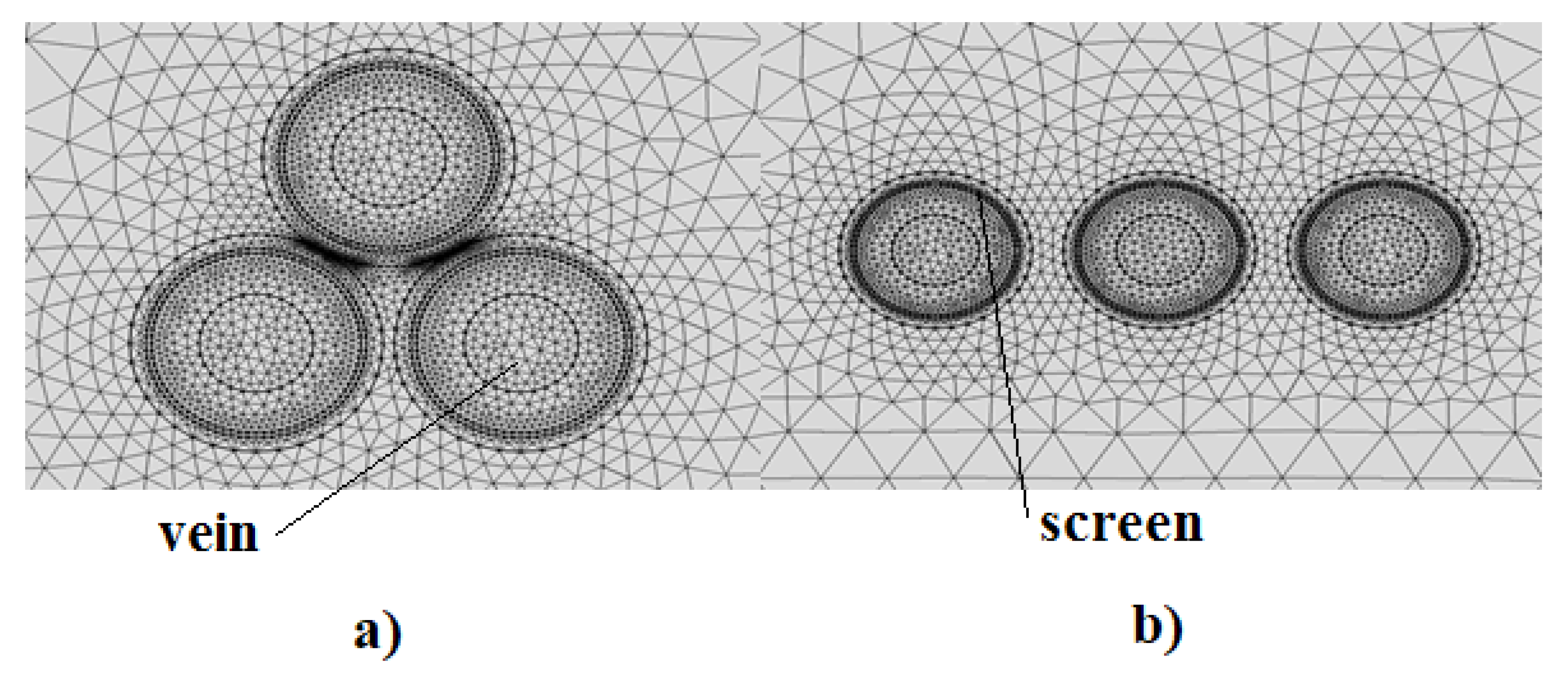
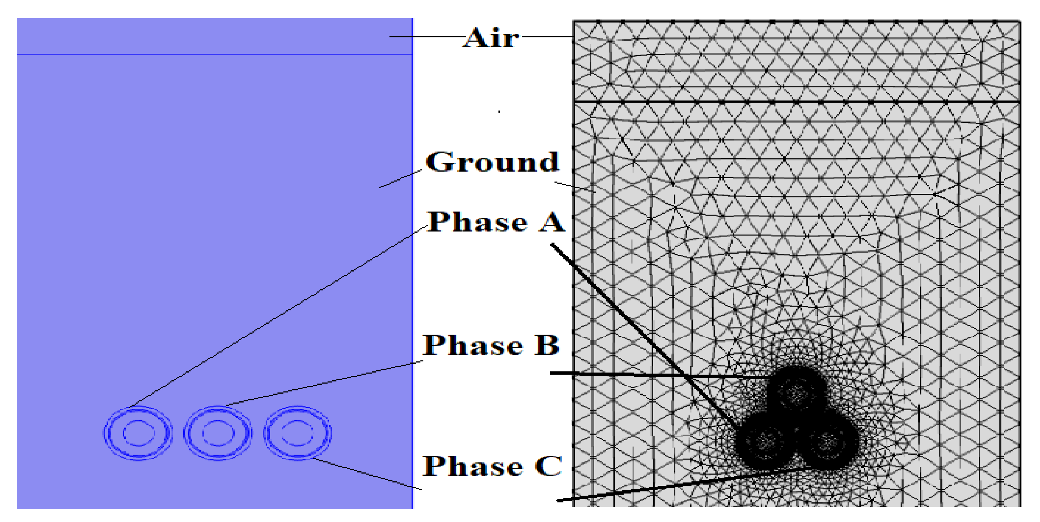
• Three different ways to build a cable line were analyzed:
  • in the ground, where the upper surfaces of the cable trench are assumed to have the same radiation properties and are filled with earth (Figure 2);
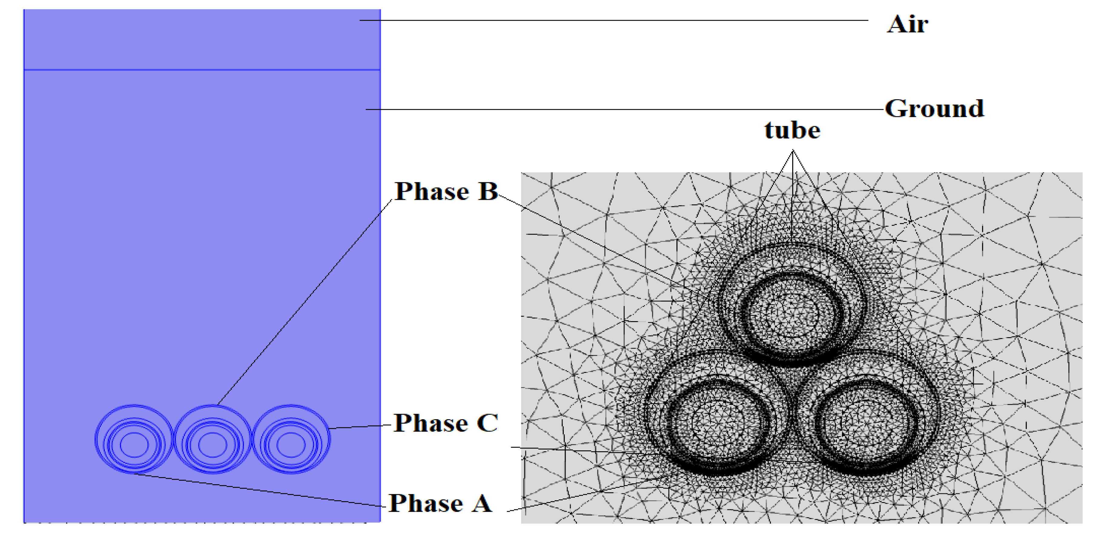
  • in tubes placed in the ground (Figure 3);
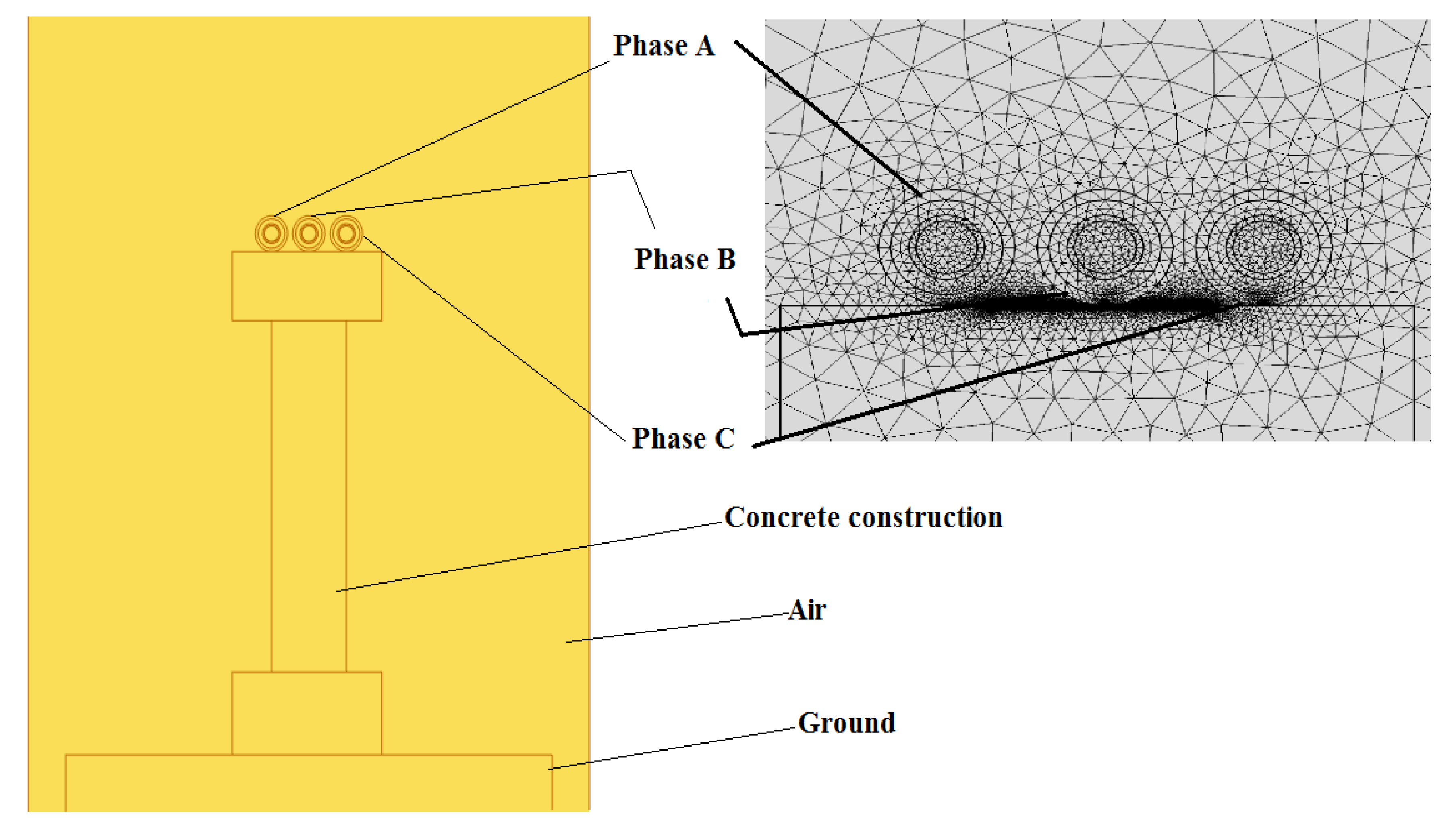
  • additionally, as part of the analysis, the variant of laying a cable line on a concrete flyover, where the cables are placed on a concrete base directly in the air, was considered (Figure 4).
• To simulate the distribution of temperature fields using the created models based on FEM, it was assumed that the cable line load for standard (normal) conditions is comparable to the rated one and for one wire it is 691 A.
• The obtained results were compared and discussed in order to develop the dependence of the new correction factor taking into account the operation of the cable line in the case of temperatures at individual points in the external environment that deviate from the standard conditions.

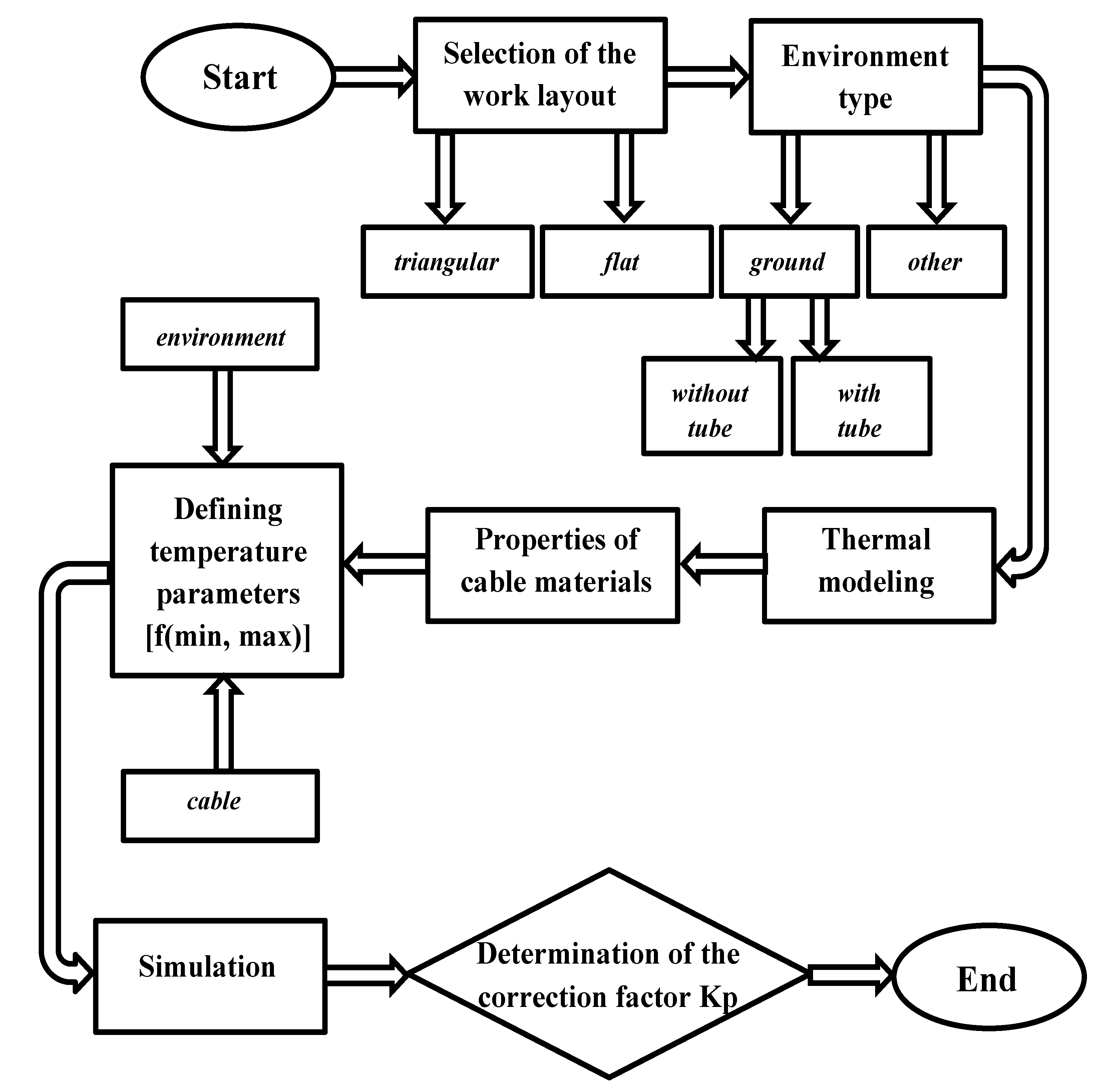
Figure 5 shows a block diagram of the proposed method for assessing the impact of changing the temperature of the external environment on the load capacity of a cable line.

The diagram reflects each step of the methodology described above. At the same time, detailed explanations of the content of the step concerning the algorithm for determining the correction factor are provided later in the article.

3. Results

3.1. Analysis of Models with Critical (Extreme) Parameters

In this part, the articles will present selected results of “extreme” test cases for the three considered ways of laying a cable line in two systems. The first case concerns the following environmental conditions: air temperature in contact with the Earth’s surface T = $-50$ ${}^{\circ }$C; the temperature of the cable core in contact with Earth is $+90$ ${}^{\circ }$C; standard parameters of materials considered in this article were adopted, soil temperature $-50$ ${}^{\circ }$C; thermal conductivity of the existing substrate around the 110 kV cable line and native soil, the values of which correspond to their dry conditions, i.e., 1 W/(m·K). Therefore, in the analyzed case, the highest possible positive temperature difference (max) of the cable line was assumed at the level of 140 ${}^{\circ }$C.

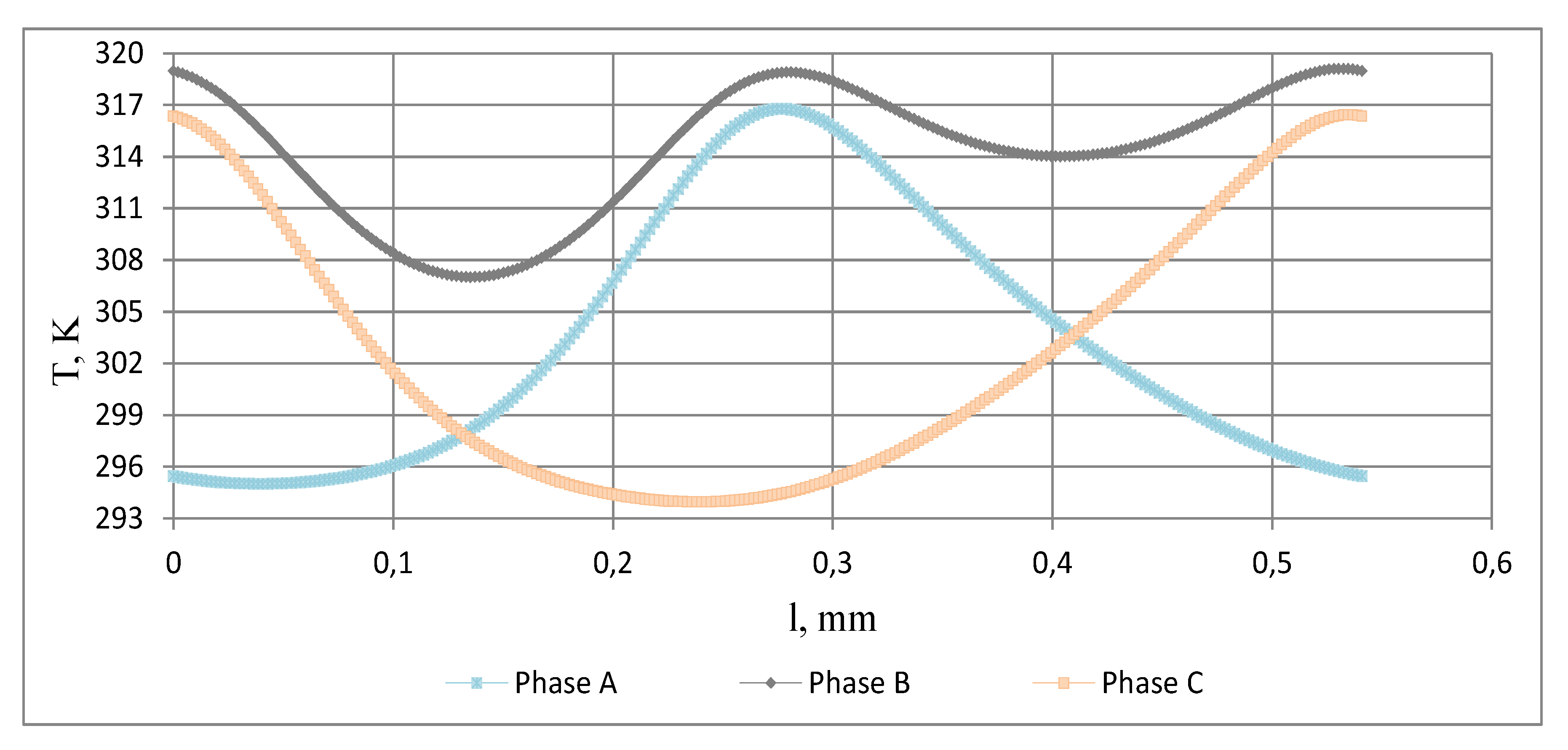
As can be seen from Figure 6, in the case of a plane system, the two extreme phases have a comparable temperature range: phase A from 293 to 316 K, and phase C from 294 to 316 K. However, the middle phase B has a much higher temperature value, which is in the range from 307 to 319 K. This situation results from the analyzed layout of the cable line. At the center, the conductor of the cable (Phase B) interacts with two end conductors of the cable (phase A and C). Moreover, the interval of the middle phase temperature change is almost two times narrower than the interval of the extreme phase change.

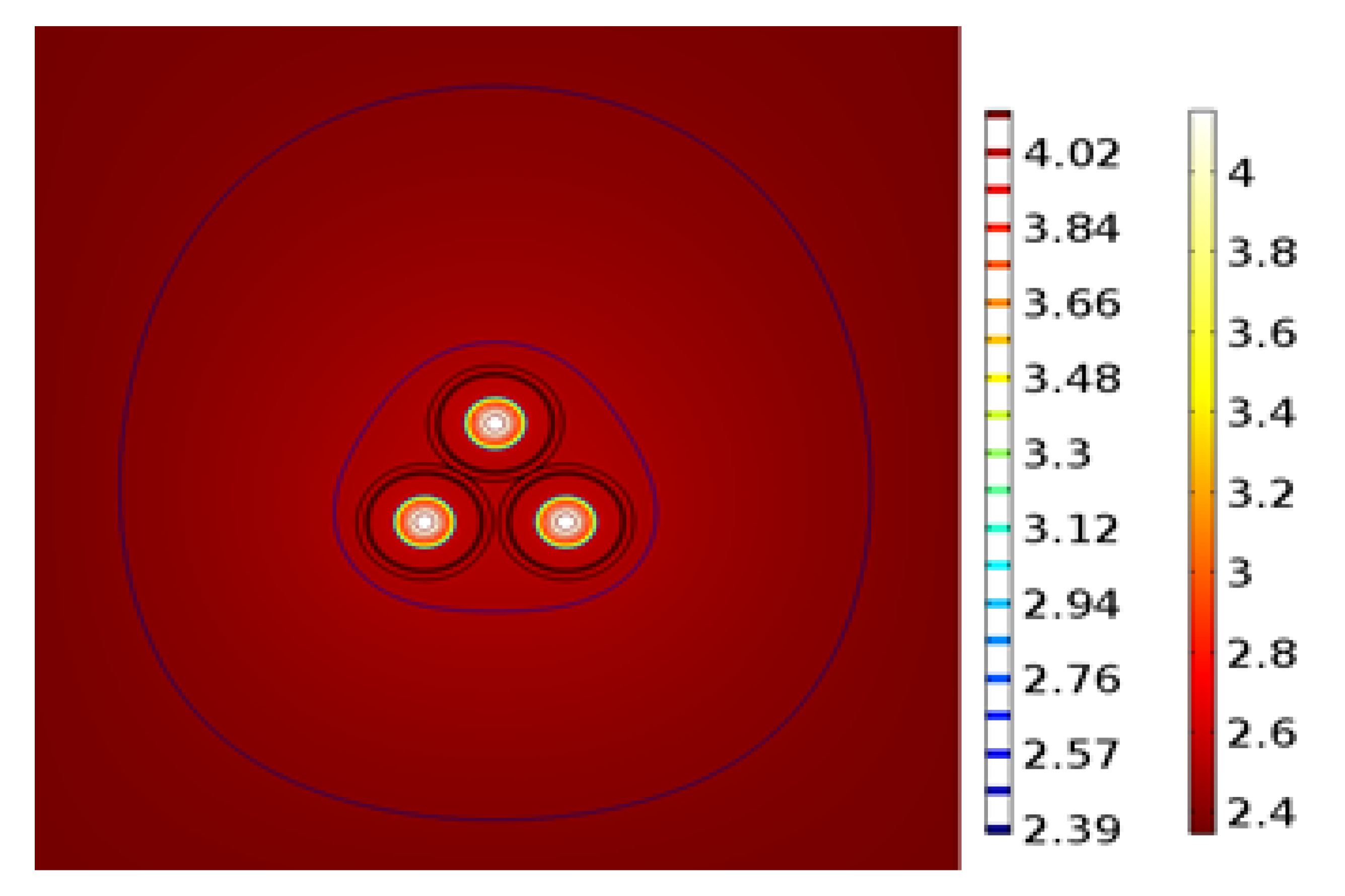
When analyzing the triangular system in Figure 7, it can be seen that the temperature situation is different than that obtained in the case of the flat system. A characteristic feature of this system in the analyzed range is that the maximum temperature for all three phases is the same and higher than the maximum temperature in the case of a flat one −332 K. At the same time, the lower limit of the temperature change range is also uniform for the three phases; but, for the extreme phases this level has a value of 314 K, and for the upper phase 317 K. Such values are also higher than the lower values of the planar range.

The second case concerns the following environmental conditions: air temperature in contact with the earth’s surface T = $+50$ ${}^{\circ }$C; the temperature of the surface of the cable in contact with the ground is $+20$ ${}^{\circ }$C; solar radiation falling on the Earth’s surface; soil temperature $+50$ ${}^{\circ }$C. Therefore, in the analyzed case, the maximum possible negative temperature difference (min) of the cable line was assumed at the level of $-30$ ${}^{\circ }$C.

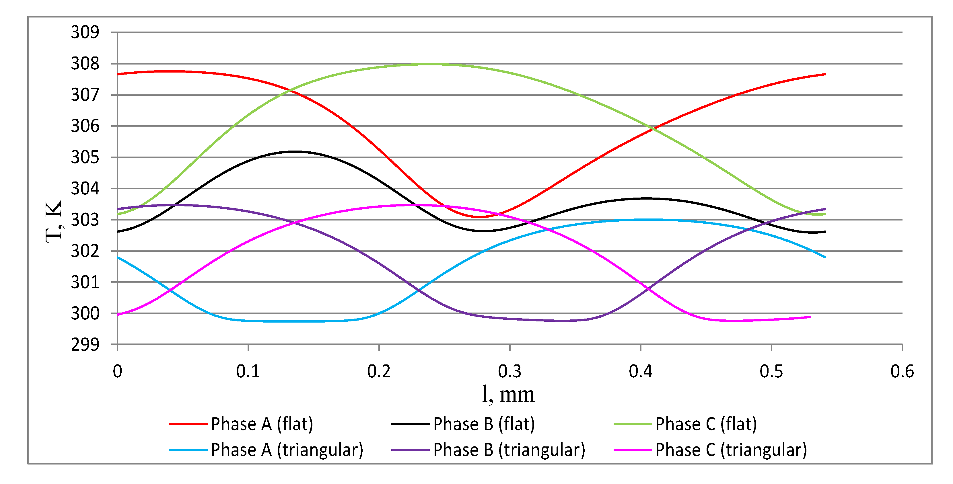
In the case of temperature distribution on the cable surface for the minimum temperature difference in the flat and triangular configuration (Figure 8), the situation differs from the previous cases. As can be seen, the range of changes for all three phases is comparable for the triangular and planar systems and is at the level of 4–5 K. The temperature between the individual phases does not differ significantly. For the flat system it is the level of 303–307 K, which is slightly higher than for the triangular system 299–303 K. This means that due to the influence of the external environment, the temperature of which is higher than the temperature of the cable core, the cable heats up to 6–10 K.

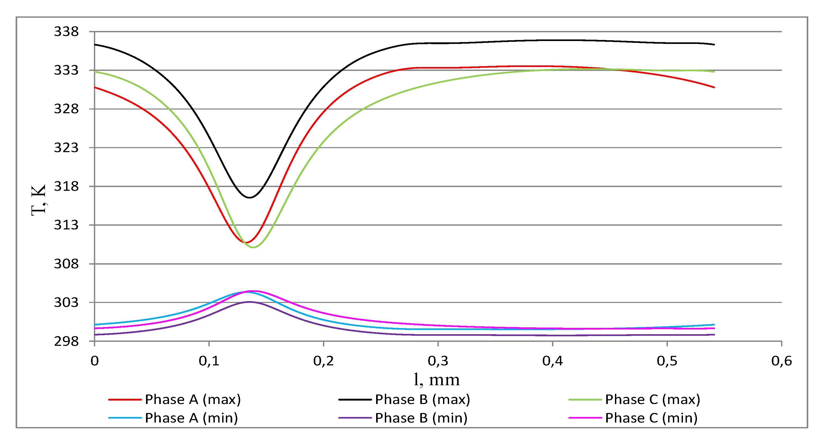
The third case concerns the environmental conditions of the first and second cases. In this case, the pipes are placed in the pipes in a flat system, which has some influence on the results (Figure 9).

When we have a situation in which the external environment has a higher temperature than the cable core, it can be seen that compared to the second case, there are lower temperatures. This value does not deviate too much and is at the level of 1–4 K. In contrast to the first case, where it was possible to observe a temperature decrease of more than 30 K with respect to the assumed level, in this case there is not a large increase in this temperature. At the same time, in the case of a maximally positive difference (140 ${}^{\circ }$C), the analyzed temperature is much higher than in the first case at the level of 16–20 K depending on the phase. On the other hand, the range of temperature change is high, but comparable to the first case.

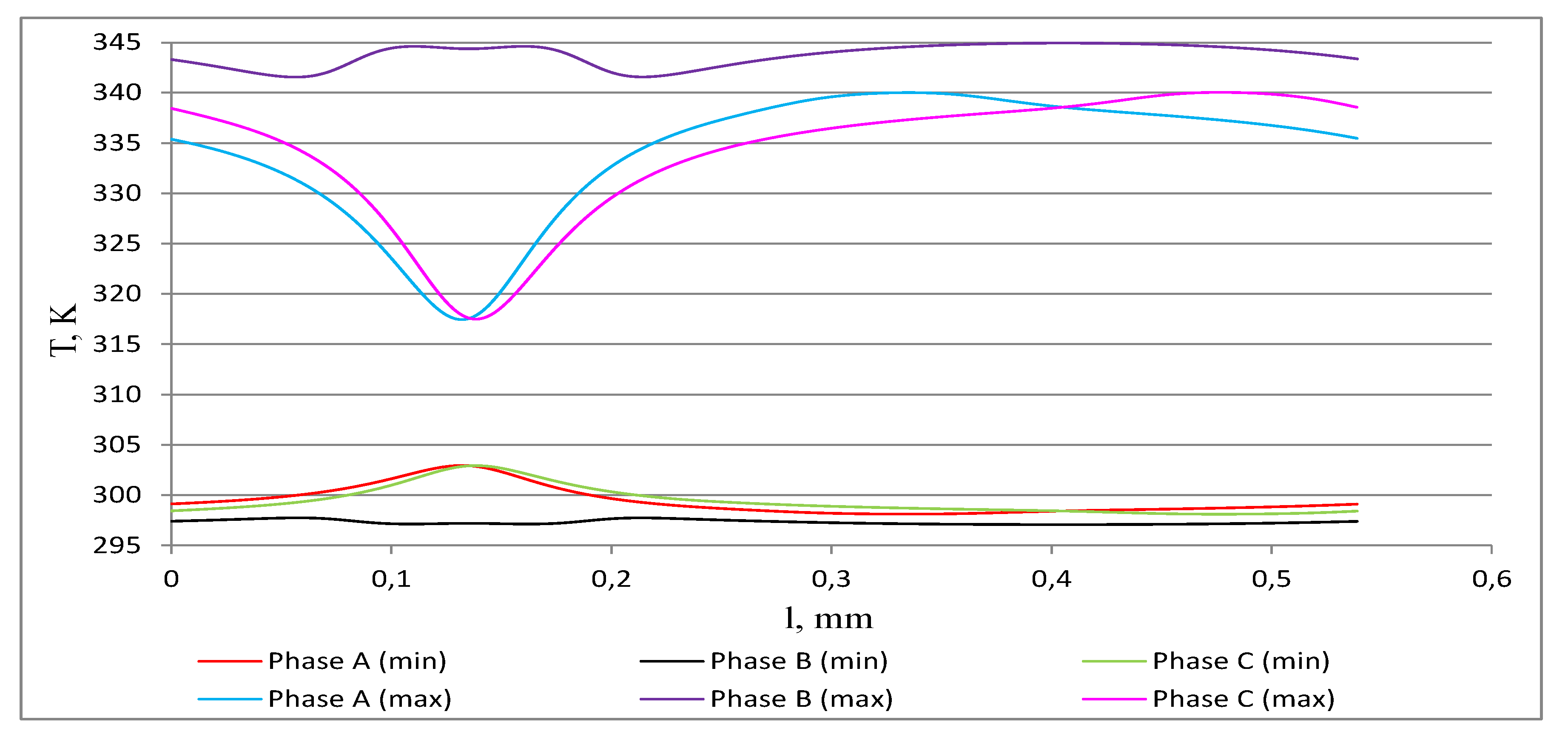
The fourth case concerned the environmental conditions that we had in the first and second cases (Figure 10). Here, for the triangular configuration of the cable placed in the pipes, a comparable length of the temperature change interval was obtained, which is 4 K. The difference is that in the middle phase at the maximum positive difference, the temperature change interval is comparable to the interval for the maximum negative temperature difference. At the same time, the triangular system has the highest temperature values of individual phases from all analyzed cases.

When the cables are laid in the air, the change in the parameters of this environment directly and in a short time affects the temperature on the surface of the cable (Figure 11). Therefore, in the case of laying the cable line in such conditions, correction factors can be applied that take into account the air temperature parameters. Therefore, this article will not consider this case in detail.

3.2. Determination of the Correction Factor for the Temperature Difference in the Cable Line

In order to work out the dependence of the change of the new correction factor, which takes into account the temperature difference between the cable line and the points of the external environment, this article proposes a formula that will allow it. To do this, first, determine the temperature difference in individual phases (4)–(6):

$$▵T_{F1}=T_{max.F1}-T_{min.F1}$$

(4)

$$▵T_{F2}=T_{max.F2}-T_{min.F2}$$

(5)

$$▵T_{F3}=T_{max.F3}-T_{min.F3}$$

(6)

As part of the task of determining the correction coefficient, we assume that the optimal temperature difference $▵T_{Fopt}$ can be described as $▵T_{Fn}$, where $F_n$ and n = 1.2,..., k—phase number, Z—task area in terms of the analyzed cable line operation system (7).

$$▵T_{Fopt}=ma{x}_{Fn\in Z}▵T_{Fn}$$

(7)

Based on the above, we can determine the component of the influence of the temperature difference (8):

$$\beta =1/▵T_{Fopt}+0.02·(T_c-T_g)$$

(8)

where $T_c$—cable core temperature, which is assumed in the range from 20 ${}^{\circ }$C to 90 ${}^{\circ }$C, $T_g$—temperature of the external environment (earth, air, etc.). The correction factor can be determined from the Formula (9) below.

$$K_p=10·(1/T_g)-0.05·\beta$$

(9)

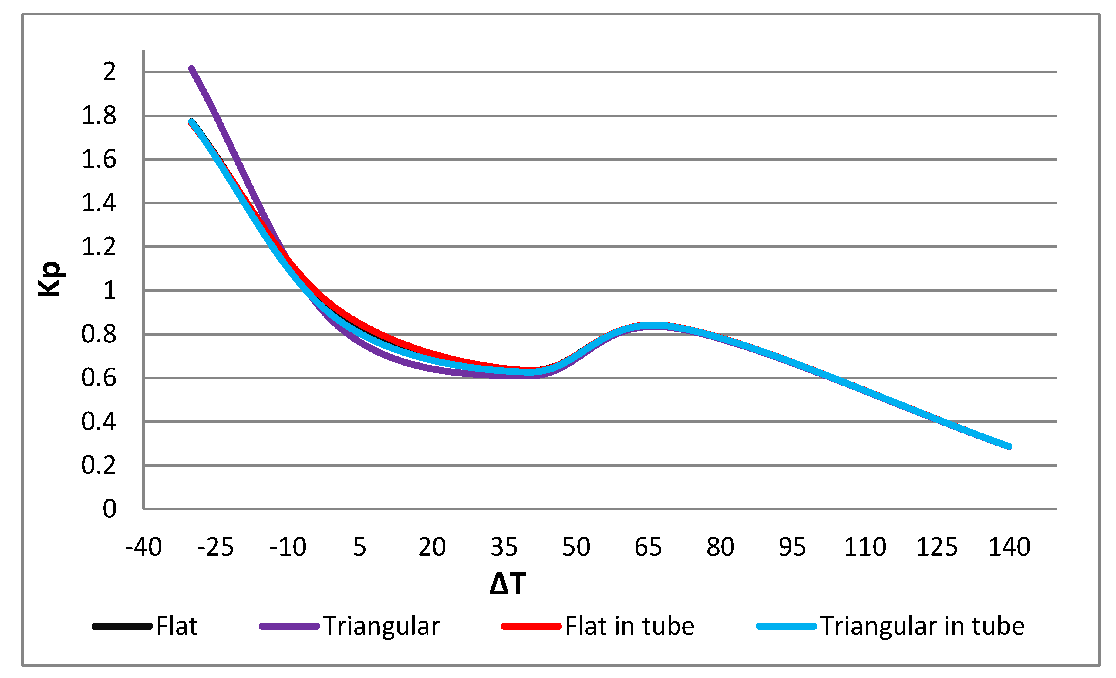
In order to be able to build the dependence of the temperature change in the cable line on the change of the temperature difference, calculations will be performed for a large number of temperature points. As part of the analysis, the analyzed correction coefficient was determined in the range from −30 K to 140 K. The developed dependence of the change of the new correction coefficient takes into account all possible cases of temperature changes at individual points of the external environment in the discussed temperature range. As can be seen from Figure 12, in the proposed range, the correction coefficient changes in the range from about 0.3 to 2. Only for the temperature difference in the range from 40 K to 100 K, there is a slight change in the downward trend into an upward trend. Such a change causes an increase (by about 0.2) of the correction factor Kp from the value of 0.6 to the value of 0.8, followed by a return to the downward trend. As can be seen, the deviation in question ends at a temperature difference of 100 K. This is due to the fact that this range is characteristic of small temperature deviations between the cable core and the external environment.

4. Model Verification and Discussion

Taking into account the permissible operating conditions of the cable core in the range from 20 ${}^{\circ }$C to 90 ${}^{\circ }$C and the permissible atmospheric conditions from $-50$ ${}^{\circ }$C to $+50$ ${}^{\circ }$C, this paper proposes a temperature difference range from $-30$ ${}^{\circ }$C to 140 ${}^{\circ }$C. This range takes into account all possible temperature cases that may occur during the operation of the cable line.

In this paper, two extreme cases were considered in detail, i.e., the temperature distribution for a maximum positive temperature difference of 140 ${}^{\circ }$C and for a maximum negative temperature difference of −30. Based on the proposed temperature difference change range, a correction factor for the temperature difference change was developed, which should be properly considered in the calculations when selecting the cable line cross-section, and which will allow to effectively take into account the unfavorable temperature differences during the cable line operation. At the same time, the existing correction factors in the environmental temperature range can be considered as auxiliary.

The comparison of the convergence of the obtained results was carried out in terms of the temperature change in the selected phase with the proposed values of the correction factor depending on the temperature difference for individual cable line systems. As can be seen from Figure 13, the change in the temperature difference between the analyzed environments leads to a comparable temperature change of the selected phase and the value of the correction factor. The greatest deviations of the correction factor occur in the extreme ranges that are characterized by the largest deviations between the temperature of the cable core and the external environment, i.e., from −30 K to 0 K and from 100 K to 140 K. The lower range of −30 K to 0 K is characteristic of a core temperature close to the nominal and an environmental temperature well above the core temperature. In contrast, the upper range from 100 K to 140 K is characterized by a core temperature close to the maximum and an environmental temperature below the core temperature.

Therefore, it can be concluded that the greater the temperature difference between the cable and the external environment, the more steep the change of the correction factor, which can be observed in the above temperature difference ranges. At the same time, it should be noted that the two ranges of the temperature difference have different limitations.

5. Conclusions

As part of this paper, a detailed analysis of the change in temperature difference between the cable core and the external environment was carried out. Simulation models were developed and the obtained results were compared depending on the different ways of laying the cable line, which affect the parameters of the considered line. The models presented in this article can lead the way for further detailed analysis of the influence of operating conditions of individual sections of the cable line.

This paper presents an algorithm for determining the correction coefficient and the development of a change curve of this coefficient in the range from about 0.3 to 2 for all possible temperature differences. The value of the correction factor has a decreasing tendency, starting with a temperature difference of −30 K. Only for the temperature difference in the range from 40 K to 100 K, there is a slight change in the downward trend into an upward trend, which has a maximum value of 0.2 at the top.

The determined correction factor was compared with the temperature change in the selected phase. It has been shown that the largest deviations of the correction factor occur in the extreme ranges that are characterized by the largest deviations between the temperature of the cable core and the external environment, i.e., from −30 K to 0 K and from 100 K to 140 K.

The obtained results, such as the correction factor variable curve, are interesting, and extensive further multi-threaded studies are possible, which are promising because they allow to increase the accuracy of the selection of cable lines without extending the time of such selection. Nevertheless, the developed factor shows that the corresponding increase in accuracy is limited depending on the temperature difference.

In conclusion, the ability to solve the problem of the safety buffer accuracy of the maximum load capacity of a cable line is a prerequisite for best practice research in the field of energy systems analysis. Instead of analyzing the influence of temperatures of individual elements of a cable line and the surrounding environment, it becomes possible to take into account the mutual influence of those parameters for which many model solutions are required. In this way, the use of effective approaches to increase accuracy greatly contributes to the emergence of well-established model-based analyzes for the development of power grid development strategies.