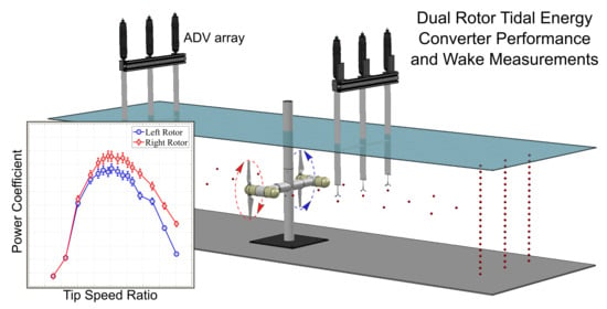
Performance and Wake Characterization of a Model Hydrokinetic Turbine: The Reference Model 1 (RM1) Dual Rotor Tidal Energy Converter

Abstract

The mechanical power and wake flow field of a 1:40 scale model of the US Department of Energy’s Reference Model 1 (RM1) dual rotor tidal energy converter are characterized in an open-channel flume to evaluate power performance and wake flow recovery. The NACA-63(4)-24 hydrofoil profile in the original RM1 design is replaced with a NACA-4415 profile to minimize the Reynolds dependency of lift and drag characteristics at the test chord Reynolds number. Precise blade angular position and torque measurements were synchronized with three acoustic Doppler velocimeters (ADV) aligned with each rotor centerline and the midpoint between the rotor axes. Flow conditions for each case were controlled to maintain a hub height velocity, $u_{hub}=$ 1.04 ms${}^{-1}$, a flow Reynolds number, $R{e}_D=$ 4.4 × 10${}^5$, and a blade chord length Reynolds number, $R{e}_c=$ 3.1 × 10${}^5$. Performance was measured for a range of tip-speed ratios by varying rotor angular velocity. Peak power coefficients, $C_P=$ 0.48 (right rotor) and $C_P=$ 0.43 (left rotor), were observed at a tip speed ratio, $\lambda =$ 5.1. Vertical velocity profiles collected in the wake of each rotor between 1 and 10 rotor diameters are used to estimate the turbulent flow recovery in the wake, as well as the interaction of the counter-rotating rotor wakes. The observed performance characteristics of the dual rotor configuration in the present study are found to be similar to those for single rotor investigations in other studies. Similarities between dual and single rotor far-wake characteristics are also observed.

1. Introduction

Growing emphasis to diversify energy portfolios, expand energy supplies and reduce carbon emissions across the globe has motivated research and development (R&D) of current energy conversion (CEC) technologies that convert the kinetic energy contained in tidal, ocean, and river currents into electricity [1]. Existing research efforts have explored a variety of CEC archetypes that include hydrokinetic turbines modeled after those developed in wind, axial- and cross-flow turbines, and unconventional devices, e.g., those using oscillating lift surfaces as prime movers [2,3]. To date, the most common hydrokinetic turbines employ axial-flow rotors. Examples include the US Department of Energy’s (DOE) Reference Model 1 (RM1) dual rotor tidal energy converter [4], an open source hydrokinetic turbine system prototype designed to benchmark techno-economic performance and support open R&D of tidal energy converters, and almost a dozen or more commercial axial-flow turbines [2,3]. Axial flow (horizontal-axis) turbines are viewed as the most proven archetype and a low risk investment for initial deployment and generation of hydrokinetic power from water currents. However, there are particular challenges transferring this proven wind turbine archetype that converts stochastic wind fields within the atmospheric surface layer to one that converts deterministic tidal currents in depth-limited boundary layer flows in the marine environment. Some of these challenges are operating in extremely corrosive environments, increased fluid density, risk of cavitation, velocity profile shear across the rotor scale, complex and potentially mobile bathymetry, and a challenging environment for installing and maintaining these devices, among others examples. Scaled model testing is still an essential research tool for performance characterization and investigating wake dynamics in turbulent geophysical flows.

Nearly a dozen studies review experimental scale model investigations of performance characteristics of single, two and three-bladed hydrokinetic turbine rotors and the factors affecting performance [5,6,7,8,9,10,11,12,13,14]. Across these experiments, rotors diameters have ranged from 0.45 m to 1.2 m [5,6,7,8,9,10,11,12,13,14,15,16,17]. Sensing capabilities in experimental models enabled observing the impact on rotor performance resulting from varying inflow turbulence intensity, unsteady loading, blade geometry, blade pitch, blade roughness (fouling), rotor yaw, submergence and cavitation, and surface waves [6,7,9,10,12,13,14,16,18]. In some cases, sensors connected to turbine blades provided unique observations of blade loads under varying operating and unsteady loading conditions [5,15,16,19,20]. Achieving Reynolds number independent performance results continues to be a challenge in small scale experiments, especially when combined with increased blockage ratios [5,17]. However, results indicate that the power coefficient, $C_P$, is more sensitive than the thrust coefficient, $C_T$, to both Reynolds number and blockage ratio [17]. To minimize this, experiments were completed at the highest blade chord length Reynolds number and lowest blockage ratio possible within the constraints of the test facility. In most cases, however, no Reynolds dependency studies were reported [5]. Blockage corrections were applied for most experiments to predict turbine performance in open water unconfined conditions [5,6,9,10,11,17]. However, uncorrected data sets are preferred for validating and verifying turbine design and analysis models [21], which can simulate the channel boundaries and blockage effects directly.

As large CEC projects require installing multiple devices in an array or turbine farm to reach commercial scale installed capacities, wake flow recovery is an important research topic for designing and operating CECs in the wake of upstream devices [22,23]. It is also important to understand the environmental effects of the wake on the environment. As noted by others, e.g., Morandi et al. 2016 [24], CEC wake interaction with the free surface and the seabed introduces unique problems with no direct analogues to wind turbine wakes. As with wind turbines, turbulence, mixing and particulate suspension are significantly increased in wake flows. For CECs, depending on the distance of the turbine rotor to the seabed, can cause local scour, re-suspension, and morphological disruptions that can affect the benthic ecology [25,26]. Within the water column, changes in the mean velocity distribution, velocity gradients and turbulence may affect the suspension and distribution of aquatic organisms, and the swimming behavior of fish and marine mammals [27,28,29,30].

Characterizing the velocity deficit, increased turbulence, and tip and hub vortex breakdown of both near-wake ($x/d_T<$ 5) and far-wake ($x/d_T>$ 5) zones remains a critical task for developing CEC technologies, especially as developers consider the economic benefits to larger, multi-turbine deployments. Fontaine et al. recently review studies characterizing wake mean and turbulent flow properties and recovery downstream of single rotor scaled model axial-flow turbines [5]. Measurements in the wake of scaled single rotor turbines highlight the complex and turbulent fluid environment. Tools such as acoustic Doppler velocimetry (ADV) [8,12,31,32,33,34,35], laser Doppler velocimetry (LDV) [5,7,24], particle image velocimetry (PIV) [5,7,10,36] and computational fluid dynamics (CFD) ranging from coupled blade element modeling (BEM) and CFD modeling of single, two and three turbine arrays [22] to high-fidelity large-eddy simulation (LES) [37,38,39] have enabled detailed descriptions of this complex wake flow, shear layer evolution, and interactions between wake vortex regions, including the breakdown of hub, tip and turbine support structure vortice [5]. A common theme has been the pronounced wake velocity deficit, a highly 3D flow structure that includes coherent hub and tip vortices, and an increase in turbulence intensity and anisotropy compared to ambient conditions. Previous studies indicate that the wake velocity deficit and turbulence recovery to upstream conditions is dependent on ambient turbulence levels, unsteady loading, turbine hub submergence depth, and turbine operating conditions affecting thrust, e.g., TSR [7,8,12,13,24,40]. Most studies indicate at least 80% flow recovery within ten diameters downstream of the rotor. Similarly, streamwise turbulence intensity levels are observed to decrease under 15% in a similar distance [7,8,12,31,32,33]. Reported values for velocity deficit and turbulence intensity among studies vary significantly in the near wake, but are relatively in good agreement in the far wake. More pronounced recovery occurs at higher ambient turbulence levels and higher blockage [7,12]. Only a few documented cases have characterized very far wake recovery beyond 15 $d_T$ [34,35,36,41].

The Reference Model Project (RMP), sponsored by the U.S. Department of Energy (DOE), created six marine energy prototypes as reference models (RMs) to benchmark performance and costs for technology developers, and to serve as non-proprietary test articles for open R&D of marine energy generation systems [4]. Open-source RMP products and supporting documentation are available at the Tethys Engineering Signature Project website (https://tethys-engineering.pnnl.gov/signature-projects/reference-model-project) to facilitate their use in future R&D studies by industry, academia, and national laboratories [42]. These products include: technical specifications and computer-aided design (CAD) files for each RM device to allow exact replication for physical and numerical modeling studies; resource site information used to design each RM device; and references to physical modeling data sets that can be used to validate numerical modeling design and analysis tools.

To our knowledge, the performance and wake characteristics of dual-rotor axial-flow tidal turbines have not been investigated in physical model experiments. The goals of the present study were to (a) evaluate dual-rotor power performance in an open-channel flow environment, (b) investigate wake flow recovery for dual-rotor axial-flow marine turbines, and (c) develop a robust data set accessible for numerical model verification and validation (V&V). A 1:40 geometrically scaled model of the U.S. DOE Reference Model 1 (RM1) dual-rotor axial flow tidal turbine system was utilized for this investigation. The design was inspired by the Seagen marine current turbine developed by Marine Current Turbines Ltd. [43] (currently acquired by SIMEC Atlantis Energy). The full-scale RM1 was designed for a 60 m deep reference tidal energy site modeled after measured inflow conditions at Tacoma Narrows and Admiralty Inlet in Puget Sound, Washington [44]. Each 20 m diameter rotor was designed with two variable-pitch NACA 631–424 hydrofoils deployed at a hub height of 30 m (mid-depth). The rotor center-to-center spacing was set at 28 m. The maximum power for each rotor is 550 kW at a rated current speed of 2.0 ms${}^{-1}$ and power coefficient of $C_p=$ 0.45. Each variable-speed power train is composed of the two-bladed rotor that drives a permanent magnet generator via a gearbox. The full dual rotor assembly can be deployed or retrieved as one unit on single support tower, potentially reducing costs associated with materials, installation, operation and maintenance. The following sections detail the design and experimental conditions for testing RM1, results on power performance and wake characteristics, including discussions comparing observations from single rotor performance and wake characterization studies.

2. Materials and Methods

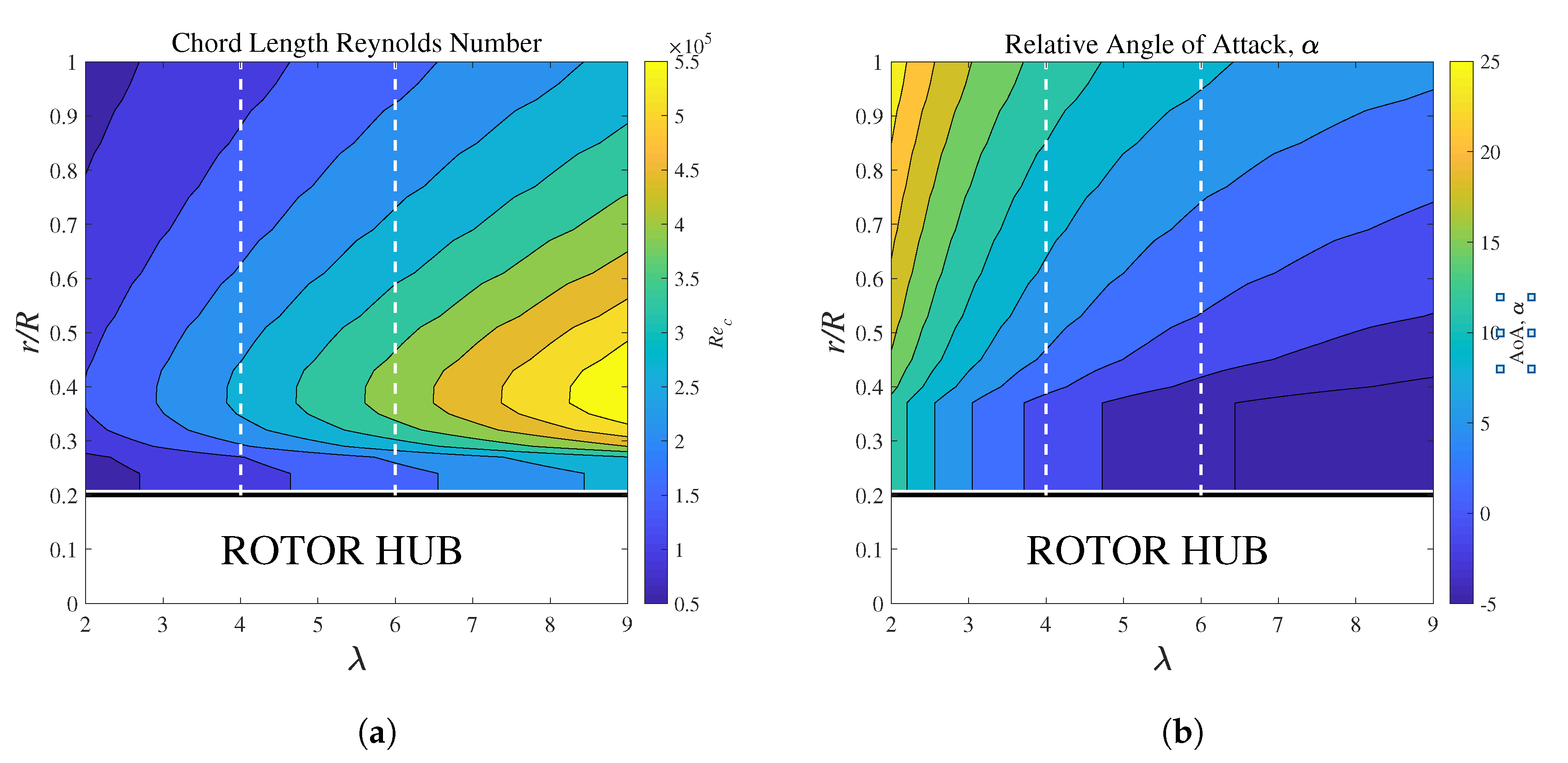
Experiments for Reference Model 1 (RM1) were completed in the Main Channel facility at St. Anthony Falls Laboratory (SAFL) at the University of Minnesota (UMN), a 2.75 m wide by 1.8 m deep by 85 m long concrete rectangular channel with controllable and continuous supply of Mississippi River water. An intake gate controls the discharge level within the flume while a mechanical tailgate weir controls flow depth, h, and monitors flow rate, $Q_w$. Water passes through two rows of vertically oriented baffles at the channel inlet to break up large scale turbulent structures before entering the test section. The SAFL Main Channel is equipped with a data acquisition (DAQ) carriage capable of three-axis automated motion. This carriage collected experimental data by positioning various sensors to monitor the hydraulic environment around a 1:40 geometric scale model of RM1 located approximately 40 m downstream of the baffles. Like the full-scale RM1, the scaled model is a dual-rotor axial flow turbine with counter-rotating rotors, each with rotor diameter $d_T=$ 0.5 m (Figure 1a). Geometric and experimental parameters are detailed in

Table 1. Experimental and Geometric characteristics of RM1 testing at SAFL. Optimal turbine efficiency, $C_{p-Opt}$, occurred at tip-speed ratio, $\lambda \approx$ 5.1. Additional turbine dimensions are available in Figure 2 and Figure 3. Rotor solidity is defined as $\sigma =Nc/\pi D$. Blockage ratio, $\eta$ = $AT/\left(hb\right)$, where $A_T$ is the combined rotor area from the two rotors and b = 2.75 m is the channel width. The Froude number is defined as $Fr=u/\sqrt{gh}$.

Parameter	1:40 Model
$Q_w$	2.425 m${}^3$s${}^{-1}$
h	1.0 m
$T_{H2O}$	18.0–20.5 °C
$u_{hub}$	1.04 ms${}^{-1}$
$Fr$	0.28
$R{e}_c$ at $C_{p-Opt}$	3.1 × 10${}^5$
$R{e}_D$	4.4 × 10${}^5$
$NACA$	4415
$d_T$	0.5 m
$h_{hub}$	0.5 m
$\sigma$	13.7%
$\eta$	14.3%
$\lambda$	1 to 9

and (Figure 2).

Instantaneous turbine power output, $P_T=\tau \omega$, from each rotor was calculated using torque, $\tau$, measurements collected by an Interface Force 20 Nm MRT miniature reaction torque sensor mounted inside each hub. Voltages from the torque transducer were transmitted to the data acquisition computer via a Rotary Systems SR003 series slip ring and Interface Force SGA signal conditioner to convert the millivolt signal to a 0-5 V range. A Pacific Scientific stepper motor (model K42HRFM-LEK-M2-00) controlled by a Parker Zeta 6108 indexer drive provided accurate and precise control of rotor angular velocity. Angular position, $\theta$, and angular velocity, $\omega$, were measured using an Automation Direct rotary encoder (model TRD-SH1000-VD) mounted to the motor shaft and referenced to the counter-rotating RM1 rotor blade position.

Velocity measurements were collected using three Nortek Vectrino+ acoustic Doppler velocimeters (ADVs) (Figure 3). All ADVs were synchronized with turbine torque and angular position measurements, enabling instantaneous turbine power coefficient calculations, $C_p=P_T/P_A$, where $P_A$ is the available power in the flow, defined as $P_A=0.5\rho A_T{\left[\overline{u_{hub}}\right]}^3$, where $\rho$ is the fluid density, $A_T$ is the swept area of the turbine rotor, and $u_{hub}$ is the instantaneous hub height velocity upstream of the turbine rotor. During performance measurements, ADVs were positioned at hub height, $h_{hub}$, three rotor diameters (3 $d_T$) upstream of the RM1 rotor location and sampled at 200 Hz for ten minutes for each rotor angular velocity. The inflow environment was further characterized by vertical velocity profiles collected at 1 $d_T$, 3 $d_T$ and 5 $d_T$ upstream of RM1. Vertical spacing was 0.05 m and measurements were collected at 200 Hz for three minutes. A horizontal velocity profile spanning the channel width at $h_{hub}$ was collected 1 $d_T$, 3 $d_T$ and 5 $d_T$ upstream of the RM1 rotors. Wake vertical velocity profiles were collected downstream of the turbine from 1 $d_T$ to 10 $d_T$ with 1 $d_T$ streamwise spacing. One ADV was aligned with the axis of rotation for each rotor ($y=\pm 0.7$$d_T$), and the third ADV was positioned at the mid-plane between the rotors centered on the vertical cylindrical support tower for RM1 (located at $y=0$$d_T$). Vertical point spacing was 0.025 m for all wake profiles and measurements were collected for five minutes at each point at 200 Hz. Additionally, a horizontal velocity plane was collected from 1 $d_T$ to 10 $d_T$ with 1 $d_T$ streamwise spacing. Cross-stream ADV point locations varied, yet provided enough spatial resolution to resolve key characteristics of the turbine wake.

2.1. Blade Design

The blade profile used for the scaled RM1 turbine design (NACA-4415) was modified from the original full-scale RM1 design blade profile (NACA-63(4)-24). Blade geometry design, performance characteristics, loading, and cavitation checks were initially performed using the BEM method code HARP-Opt developed at the National Renewable Energy Laboratory (NREL). Model scale blades for RM1 were redesigned to NACA-4415 due to a lower Reynolds number during experiments and availability of low Reynolds number lift ($C_L$) and drag ($C_D$) coefficient data.

Table A1. Characteristics of RM1 turbine blades (NACA-4415). A circular blade root was used to allow for manual pitch control.

$\mathit{r}/\mathit{R}$	$\mathit{c}/\mathit{R}$	$\mathit{t}/\mathit{c}$	$\mathit{\alpha }{(}^{°})$
0.21	0.12	1.00	13.16
0.24	0.12	1.00	13.16
0.27	0.14	0.85	13.16
0.29	0.19	0.52	13.16
0.32	0.23	0.31	13.16
0.35	0.25	0.19	13.16
0.37	0.26	0.15	13.16
0.40	0.26	0.15	11.28
0.43	0.25	0.15	10.24
0.45	0.25	0.15	9.43
0.48	0.24	0.15	8.76
0.51	0.23	0.15	8.17
0.53	0.22	0.15	7.64
0.56	0.21	0.15	7.16
0.59	0.21	0.15	6.70
0.61	0.20	0.15	6.27
0.64	0.19	0.15	5.86
0.67	0.18	0.15	5.46
0.69	0.18	0.15	5.07
0.72	0.17	0.15	4.69
0.75	0.16	0.15	4.31
0.77	0.16	0.15	3.93
0.80	0.15	0.15	3.55
0.83	0.15	0.15	3.17
0.85	0.14	0.15	2.78
0.88	0.14	0.15	2.38
0.91	0.13	0.15	1.98
0.93	0.13	0.15	1.57
0.96	0.13	0.15	1.14
1.00	0.12	0.15	0.70

in Appendix A provides details of the blade geometry, while comparisons between full-scale geometry of the original RM1 blade profile and the re-designed NACA-4415 blades are illustrated in Figure 4.

Laboratory-scale models are tested at a much lower Reynolds numbers compared to the full-scale system. This can result in unrealistic lift and drag coefficients that vary compared to the field-scale system counterpart. To determine these differences for the RM1 model tested in this study, XFOIL static models were run to compare aerodynamic coefficients. First, 2D vector flow analysis was modeled to calculate a matrix of model scale chord length Reynolds numbers and local angle-of-attack as a function of tip-speed ratio and local blade element radius (Figure 5). Model-scale mid-span and tip $R{e}_c$ ranged from 1.7 × 10${}^5$ to 3.0 × 10${}^5$ in the range of $\lambda =$ 4–6 where measurements indicated optimal performance (Figure 5a). Similarly, relative angle-of-attack (i.e., the blade angle-of-attack with respect to the resultant velocity vector from the inflow velocity and local blade element velocity) ranged from $\alpha =$ 2°–9° when the blade pitch was set to 0° (Figure 5b).

A closer inspection of the predicted lift and drag coefficients at these angles is found in Figure 6. XFOIL simulations were completed for chord length Reynolds number at both model scale ($R{e}_c=$ 8.2 × 10${}^4$ to 2.7 × 10${}^5$ for $\lambda =$ 2 to 9, respectively) and field scale ($R{e}_c=$ 6.8 × 10${}^6$ to 2.2 × 10${}^7$ for $\lambda =$ 2 to 9, respectively. $N_{crit}=$ 5 for all cases.). Model-to-Field scale lift coefficient ratios ranged from 1.0–1.2 within the predicted relative angles-of-attack for $\lambda =$ 4–6 (Figure 6a). Similarly, Model-to-Field scale drag coefficient ratios were approximately 2.0 within the predicted relative angle-of-attacks for these optimal tip-speed ratios (Figure 6b). Given that the torque generating component ratio ($C_{L-model}/C_{L-field}$) is approximately 1.0 between model and field scales, we anticipate the measured performance of the RM1 scaled turbine to be within the Reynolds number independent regime where measured performance characteristics no longer change with increasing Reynolds number.

2.2. Data Reduction Methods

The following parameters were calculated during the processing of the velocity and turbine performance data collected during the RM1 experiments at SAFL. The 200 Hz velocity data output from the three Nortek Vectrino+ velocimeters were filtered to remove any erroneous data [45]. Through Reynolds decomposition, the velocity timeseries can be decomposed into the mean and fluctuation components,

$$u_i=\overline{u}+u^{\prime }$$

(1)

The so calculated fluctuating velocity components are then used to calculate a number of flow statistics. The turbulence intensities are dimensionless parameters that describe the level of turbulence within the flow along each spatial direction and are defined as the root-mean squared of the fluctuating velocity component divided by the mean velocity magnitude, where,

$${\overline{u}}_M=\sqrt{{\overline{u}}^2+{\overline{v}}^2+{\overline{w}}^2}$$

(2)

and,

$$I_{u_i}=\sqrt{\overline{{u_i^{\prime }}^2}}/\overline{u_M}$$

(3)

for $u_i=$$u,v,w$. The Reynolds stress tensor is defined as follows:

$${\tau }_{ij}=\overline{u_i^{\prime }{u}_j^{\prime }}$$

(4)

When $i=j$, the results are the normal stresses ($\overline{u^{\prime }{u}^{\prime }}$, $\overline{v^{\prime }{v}^{\prime }}$, $\overline{w^{\prime }{w}^{\prime }}$), also known as the velocity variance, ${\sigma }_{u_i}^2$, and when $i\ne j$, the results are the shear stresses ($\overline{u^{\prime }{v}^{\prime }}$, $\overline{u^{\prime }{w}^{\prime }}$, $\overline{v^{\prime }{w}^{\prime }}$). The turbulence kinetic energy (TKE), k, is defined as follows:

$$k=\frac{1}{2}\left(\overline{u^{\prime }{}^2}+\overline{v^{\prime }{}^2}+\overline{w^{\prime }{}^2}\right)$$

(5)

The streamwise velocity deficit is a common metric used to report the wake velocity recovery downstream of a turbine, and is defined as follows:

$$u_{def}=\frac{\left|u_{hub}-u_x\right|}{u_{hub}}$$

(6)

where $u_{hub}$ is the upstream approach velocity at $h_{hub}$ and $u_x$ is the hub height velocity at position x downstream of the turbine. Here, $u_{hub}$ is measured at $x/d_T=$−5.

As previously mentioned, using synchronous velocity, torque and rotor position measurements, various turbine parameters could be calculated. The rotor position was used to calculate the turbine angular velocity, $\omega$. Turbine power, $P_T$, was calculated using the measured torque and angular velocity using,

$$P_T=\tau \omega$$

(7)

where $\tau$ is the measured torque and $\omega$ is the defined and verified angular velocity that was applied via the stepper motor and measured using the positional encoder integrated with the drive system. The available power within the approaching flow was calculated using the synchronous velocity measurements upstream of the RM1 location using,

$$P_A=\frac{1}{2}\rho A_T{\left(\overline{u_{hub}}\right)}^3$$

(8)

where $P_A$ is the calculated available power, $\rho$ is the fluid density (≈1 kg m${}^{-3}$) dependent on water temperature (typically between 18.0 °C and 20.5 °C during RM1 tests), $A_T$ is the flow cross sectional area covered by the device ($A_T=\left(\pi {d_T}^2\right)/4$), and ${\overline{u}}_{hub}$ is the time average of the approach flow instantaneous velocity measurements using three ADVs at hub height 3 $d_T$ upstream of RM1. Using these power calculations, the turbine power coefficient, $C_p$, is calculated using the equation,

$$C_p=\frac{P_T}{P_A}$$

(9)

This parameter describes the fraction of power extracted from the approaching flow by the turbine. An additional dimensionless parameter used to describe the turbine performance characteristics is the tip-speed ratio, $\lambda$, defined as the ratio of the rotor tip speed to the speed of the approaching flow,

$$\lambda =\frac{\omega d_T}{2\overline{u_{hub}}}$$

(10)

2.3. Uncertainty Analysis

In experimental measurements, both systematic and random measurement error exists [46]. Systematic error in the torque sensors was determined during torque sensor calibration by applying known torque values and comparing measured against expected values. Results of the calibration tests represent the systematic error associated with the torque sensors during RM1 experiments. This systematic error was removed prior to calculating and reporting of experimental measurement uncertainty. Uncertainty values for the ADVs and optical encoder were used from the manufacturer’s reported values and incorporated into error propagation from measurements into calculations of turbine performance, $C_p$. Additionally, extended datasets were collected to assess the uncertainty in mean values of each instrument. The results showed that uncertainty in the torque, $\tau$, was ${\Delta }_{\tau }/\tau =$ 1.92%. Uncertainty in angular velocity, $\omega$, was ${\Delta }_{\omega }/\omega =$ 2.5%. Uncertainty in velocity measurements, u, was ${\Delta }_u/u=$ 0.78%. Methods outlined by Coleman and Steele [46] were used to calculated the combined uncertainty from measured variables used in calculating $C_p=$ f($\tau$, $\omega$, $u^3$). Uncertainty in calculated $C_p$ values is given by;

$${\frac{{\Delta }_{C_p}}{C_p}}^2={\frac{{\Delta }_{\tau }}{\tau }}^2+{\frac{{\Delta }_{\omega }}{\omega }}^2+{\left(-3\right)}^2{\frac{{\Delta }_{\overline{u}}}{\overline{u}}}^2$$

(11)

Using the uncertainty values reported above, the uncertainty in calculated $C_p$ values is approximately ${\Delta }_{C_p}\approx$ 3.9%.

3. Results

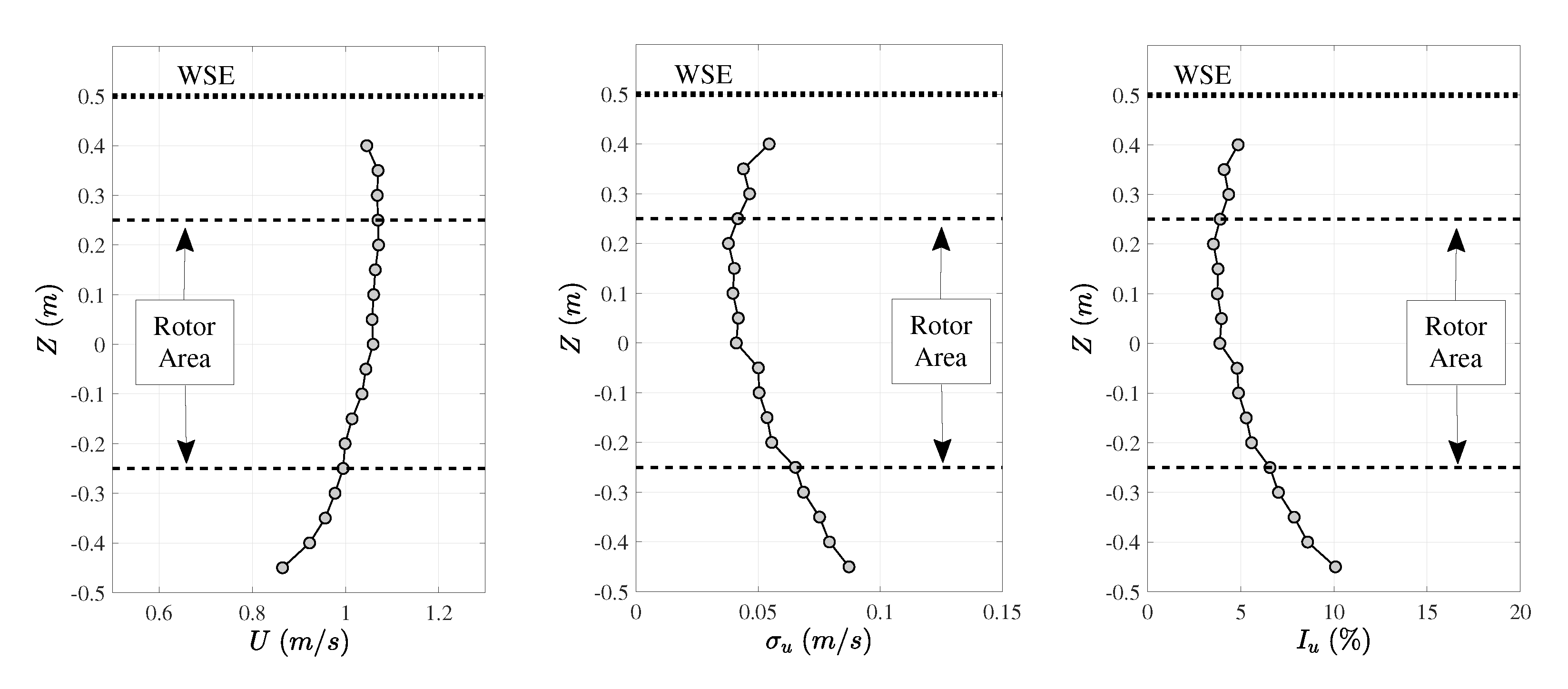
3.1. Inflow Characteristics

Vertical and horizontal inflow velocity profiles were collected 3 $d_T$ (1.5 m) and 5 $d_T$ (2.5 m) upstream of RM1 (Figure 7 and Figure 8). Average hub height streamwise velocity, $\overline{u_{hub}}=$ 1.04 ms${}^{-1}$, while turbulence intensity across the rotor swept region was approximately 5%. The shear velocity, $u_{*}$, in open channel flow is an important parameter in characterizing the near-wall stresses imposed by the flow on the channel boundaries. This parameter can be estimated using velocity profiles and the logarithmic law of the wall equation,

$$\frac{\overline{u}}{u_{*}}=\frac{1}{\kappa }ln\left(\frac{z}{z_0}\right)$$

(12)

where $\overline{u}$ is the mean velocity at z, the distance from the wall, $\kappa$ is the von Kármán constant ($\kappa$ = 0.41), and $z_0$ is the hydrodynamic roughness length. Using this method, the friction velocity was found to be, $u_{*}=$ 0.033 ms${}^{-1}$. The SAFL main channel facility is hydraulically smooth, so the resulting hydrodynamic roughness length, $z_0\approx$ 1 $\times {}^{-6}$ m.

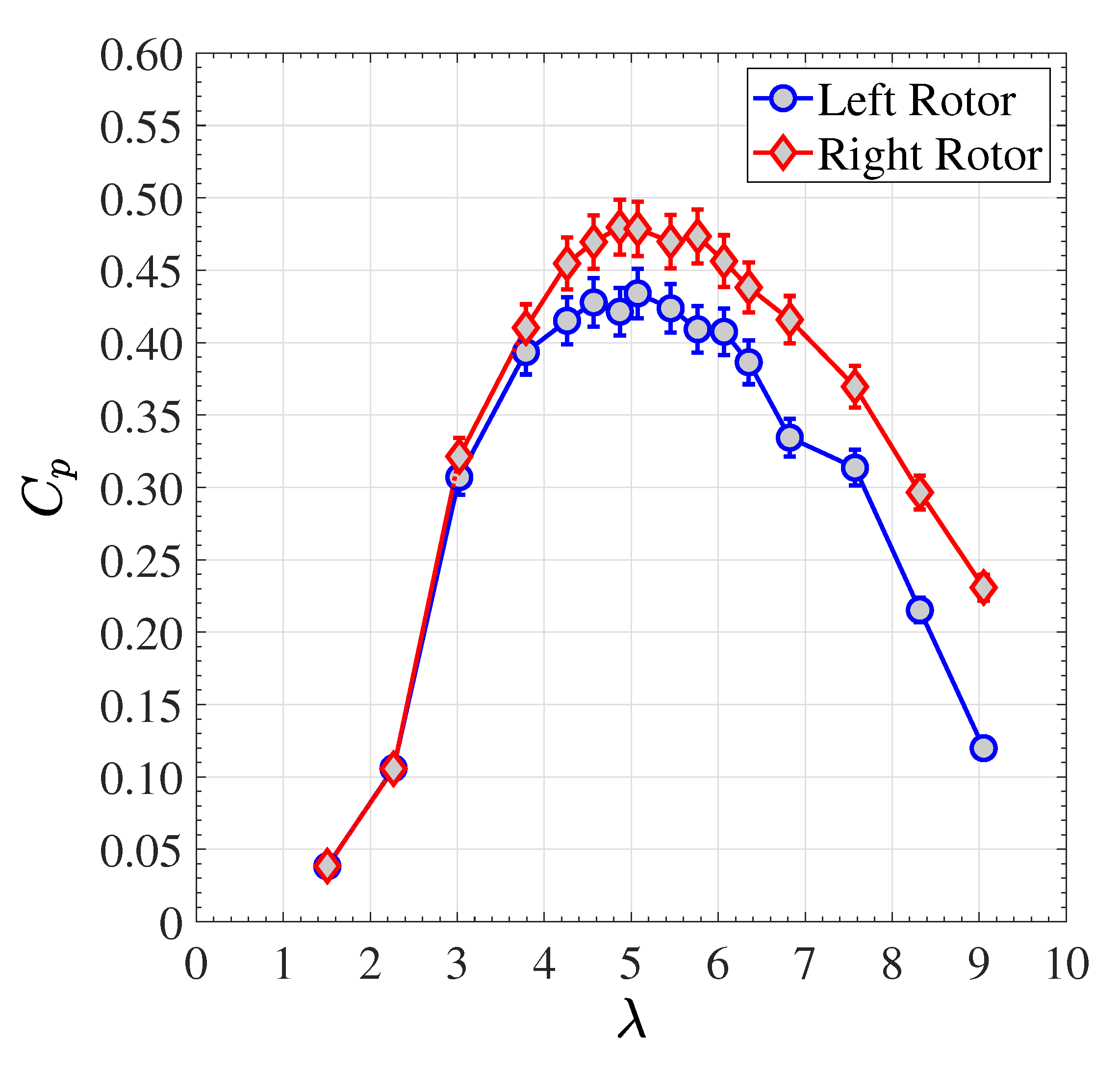
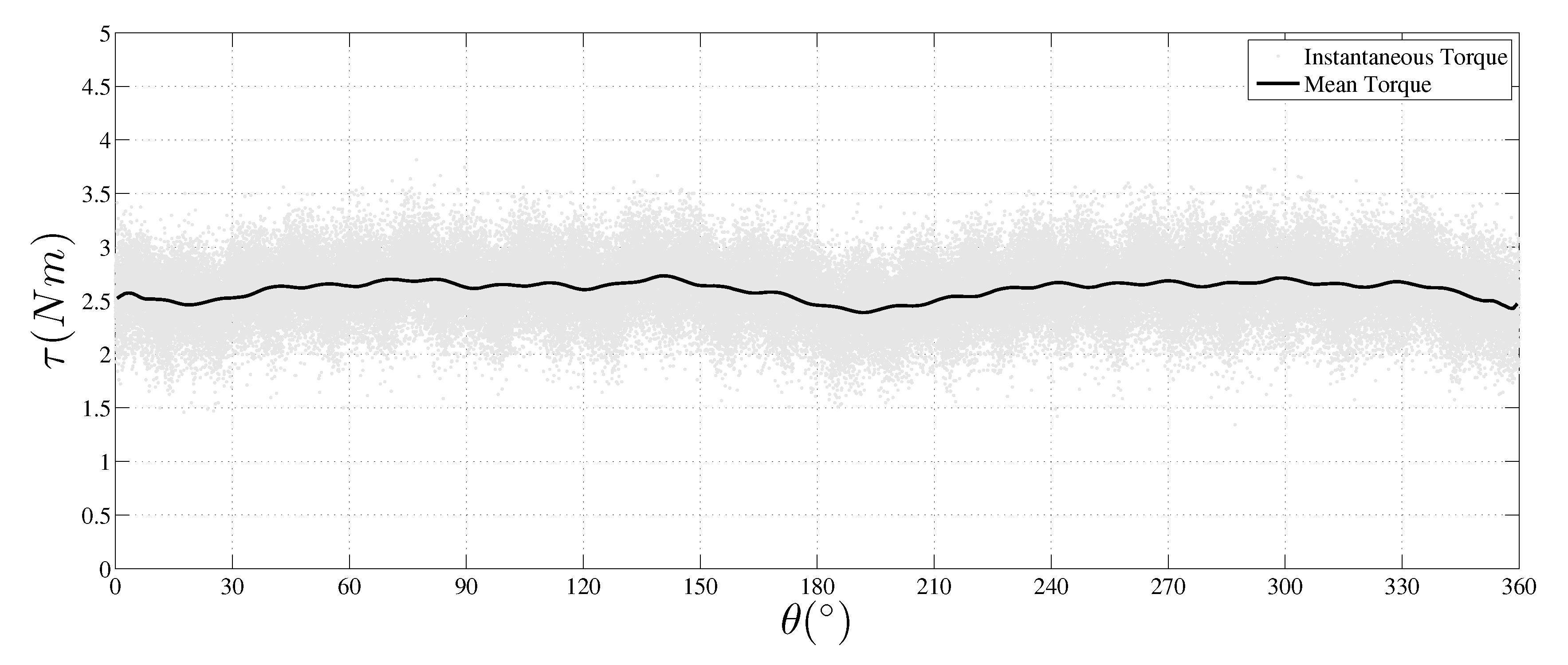
3.2. Turbine Performance

Performance curves for both the left and right RM1 rotors are shown in Figure 9. The data use for this figure, including rotor RPM (revolutions per minute), measured torque, $\tau$, inflow characteristics, and calculated quantities ($\lambda$, $P_A$, $P_T$, $I_u$, k, and $C_p$) are available for both the right and left rotors in Appendix B,

Table A2. Performance testing conditions and summary—RM1 right rotor, $y/d_T=$ 0.7.

$\mathit{RPM}$	$\mathit{TSR}$	$\mathit{\tau }\left(\mathbf{Nm}\right)$	${\mathit{P}}_{\mathit{T}}\left(\mathit{W}\right)$	$\mathit{U}(\mathit{m}/\mathit{s})$	$\mathit{V}(\mathit{m}/\mathit{s})$	$\mathit{W}(\mathit{m}/\mathit{s})$	${\mathit{I}}_{\mathit{u}}(\%)$	$\mathit{k}({\mathit{m}}^2/{\mathit{s}}^2)$	${\mathit{P}}_{\mathit{A}}\left(\mathit{W}\right)$	${\mathit{C}}_{\mathit{P}}$
60	1.50	0.69	4.32	1.050	−0.010	0.008	4.05	0.0026	114.03	0.038
90	2.25	1.25	11.73	1.048	−0.011	0.006	4.79	0.0031	113.49	0.106
120	2.99	2.86	35.94	1.050	−0.011	0.003	4.89	0.0031	114.22	0.321
150	3.76	2.88	45.24	1.045	−0.010	0.005	4.92	0.0031	112.63	0.410
168	4.22	2.83	49.73	1.042	−0.012	0.003	4.89	0.0030	111.63	0.455
180	4.54	2.70	50.92	1.039	−0.008	0.003	4.87	0.0029	110.69	0.469
192	4.85	2.57	51.68	1.037	−0.009	0.004	5.04	0.0031	110.06	0.480
204	5.03	2.62	53.51	1.052	−0.011	0.002	5.16	0.0034	111.71	0.479
216	5.40	2.31	52.24	1.048	−0.010	0.000	4.86	0.0030	113.44	0.470
228	5.74	2.15	51.35	1.040	−0.012	0.000	5.11	0.0032	110.95	0.473
240	6.04	1.97	49.61	1.041	−0.010	−0.003	5.25	0.0033	111.36	0.456
252	6.32	1.84	48.60	1.045	−0.010	−0.003	3.53	0.0023	112.08	0.438
270	6.77	1.62	45.78	1.044	−0.012	−0.008	4.78	0.0028	112.22	0.416
300	7.52	1.30	40.72	1.044	−0.011	−0.007	5.00	0.0029	112.46	0.370
330	8.28	0.94	32.63	1.044	−0.011	−0.007	4.71	0.0028	112.11	0.296
360	9.01	0.68	25.60	1.046	−0.011	−0.008	4.55	0.0022	112.83	0.231

and

Table A3. Performance testing conditions and summary—RM1 left rotor, $y/d_T=$ −0.7.

$\mathit{RPM}$	$\mathit{TSR}$	$\mathit{\tau }\left(\mathbf{Nm}\right)$	${\mathit{P}}_{\mathit{T}}\left(\mathit{W}\right)$	$\mathit{U}(\mathit{m}/\mathit{s})$	$\mathit{V}(\mathit{m}/\mathit{s})$	$\mathit{W}(\mathit{m}/\mathit{s})$	${\mathit{I}}_{\mathit{u}}(\%)$	$\mathit{k}({\mathit{m}}^2/{\mathit{s}}^2)$	${\mathit{P}}_{\mathit{A}}\left(\mathit{W}\right)$	${\mathit{C}}_{\mathit{P}}$
60	1.50	0.66	4.18	1.044	−0.006	0.010	5.35	0.0034	112.36	0.038
90	2.27	1.21	11.34	1.036	−0.004	0.010	5.45	0.0036	109.81	0.106
120	3.03	2.61	32.82	1.036	−0.004	0.014	5.67	0.0038	109.90	0.307
150	3.79	2.68	42.06	1.036	−0.004	0.010	5.72	0.0038	109.90	0.394
168	4.26	2.50	43.92	1.032	−0.005	0.012	5.73	0.0037	108.70	0.415
180	4.57	2.40	45.29	1.032	−0.005	0.010	5.67	0.0037	108.76	0.428
192	4.85	2.24	45.11	1.036	−0.005	0.009	5.52	0.0036	109.84	0.422
204	5.07	2.31	48.18	1.039	−0.004	0.008	5.79	0.0040	111.01	0.434
216	5.47	1.99	45.10	1.034	−0.004	0.007	5.49	0.0035	109.17	0.424
228	5.75	1.85	44.19	1.038	−0.004	0.007	5.49	0.0034	110.53	0.409
240	6.06	1.74	43.73	1.036	−0.005	0.008	5.58	0.0035	110.05	0.408
252	6.34	1.59	42.00	1.040	−0.004	0.006	5.26	0.0032	111.24	0.387
270	6.82	1.27	36.03	1.037	−0.002	0.004	5.08	0.0030	110.01	0.335
300	7.59	1.07	33.53	1.035	−0.003	0.005	5.41	0.0032	109.44	0.314
330	8.32	0.68	23.34	1.039	−0.005	0.001	5.20	0.0031	110.73	0.215
360	9.05	0.35	13.03	1.041	−0.005	0.001	4.99	0.0029	111.30	0.120

, respectively. The best operating points for both rotors occurred at approximately $\lambda$ = 5.1. However, the maximum power coefficients ($C_{p-max}$) differed, with a $C_{p-max}$ = 0.48 for the right rotor and $C_{p-max}$ = 0.43 for the left rotor. As mentioned previously, instantaneous torque and angular position measurements provided a method for investigated azimuth specific torque production from each rotor (Figure 10). RM1 blades are offset 180° on each rotor but were counter-rotating in symmetry. Due to the large diameter cylindrical shape of the horizontal support arm ($d_{arm}=$ 0.076 m, $d_{arm}/d_T=$ 15%) extending to each rotor from the center support tower, a noticeable decrease of approximately 5–10% in the average torque production is observed as the blades pass azimuthal positions $\theta \approx$ 0° and 180°.

Thrust forces were not directly measured during the scaled RM1 dual-rotor experiments; however, an estimate of the rotor thrust coefficient was calculated based on momentum theory using flow-field velocity measurements at hub-height immediately upstream ($x/d_T=$−1) and downstream of the turbine ($x/d_T=$ 1). The results indicate the rotors were operating with a thrust coefficient, $C_T\approx$ 0.52, at the optimal tip speed ratio.

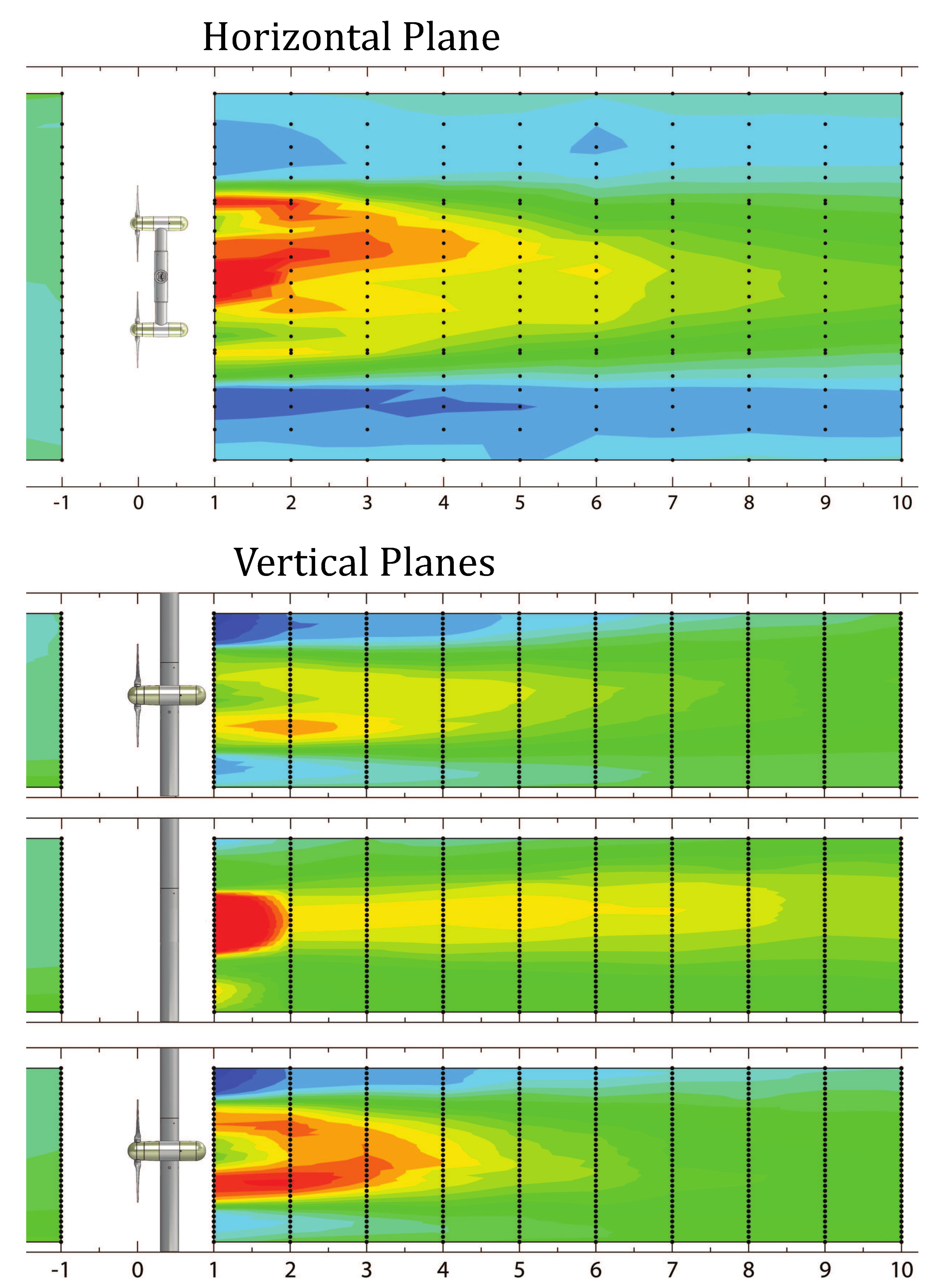
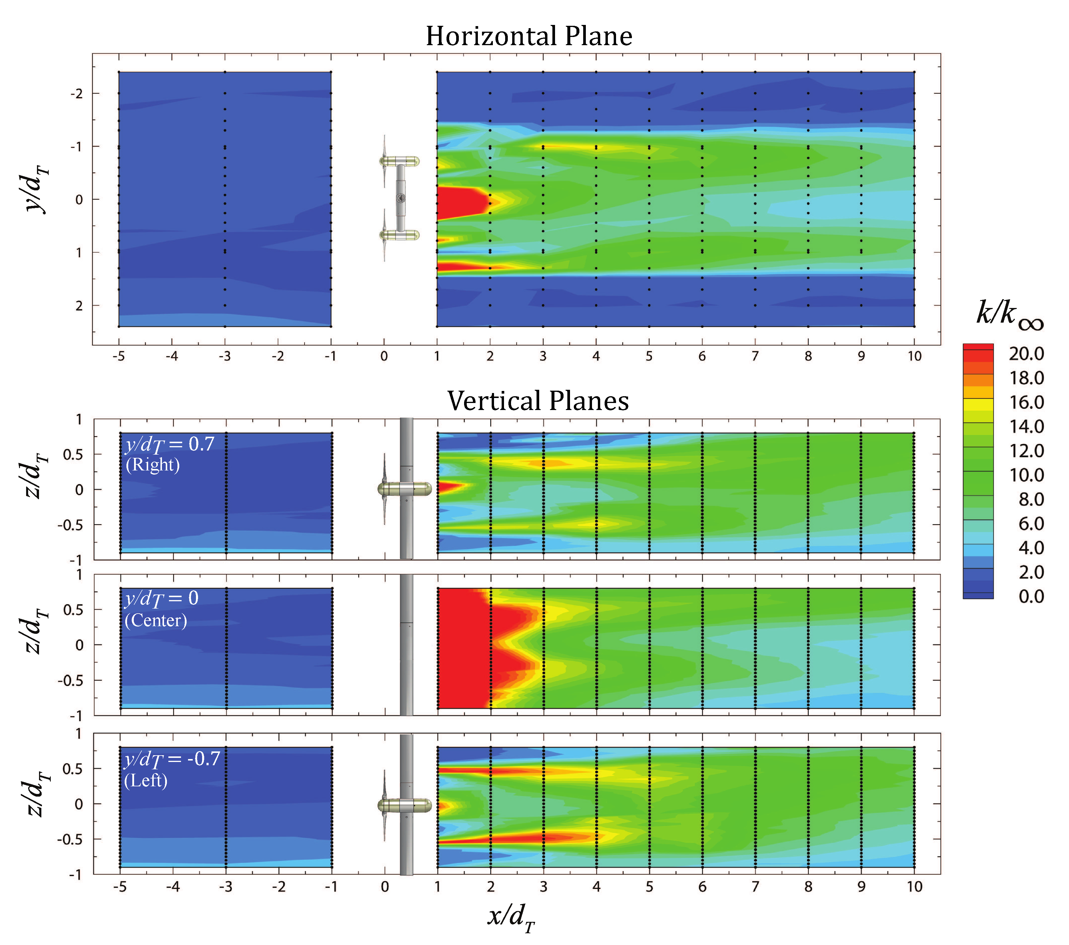
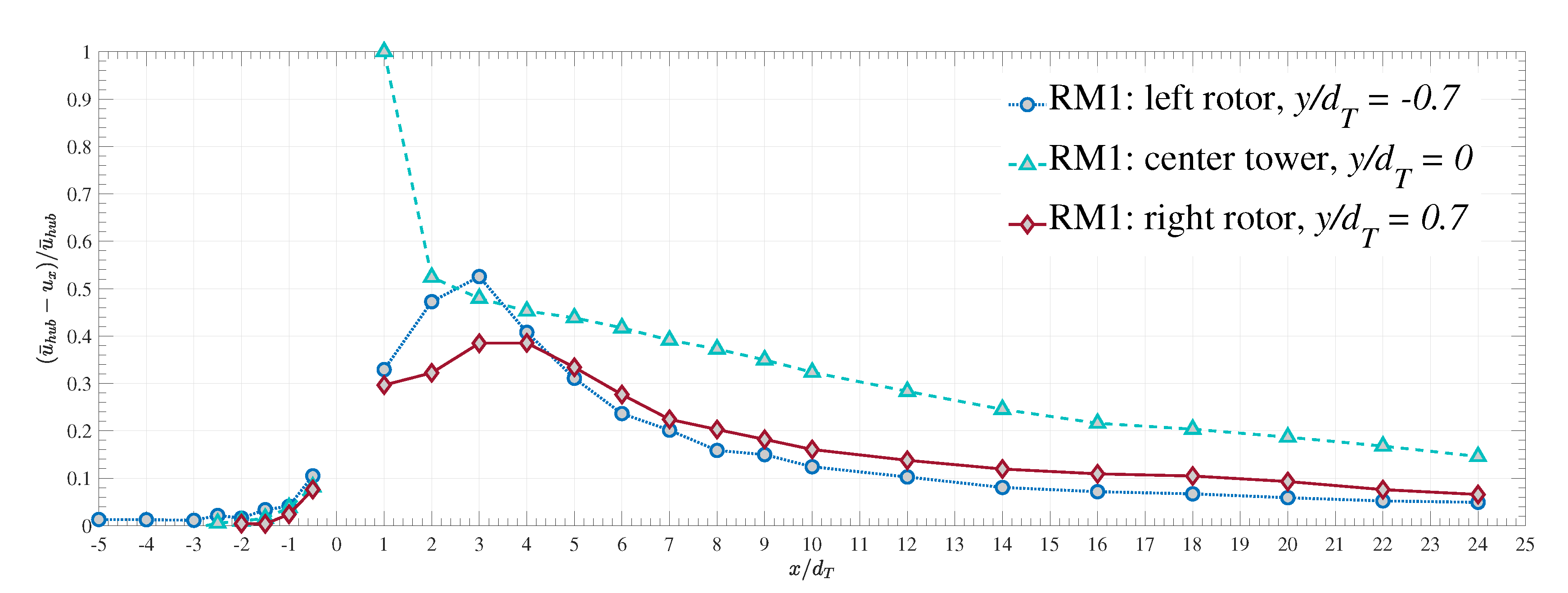
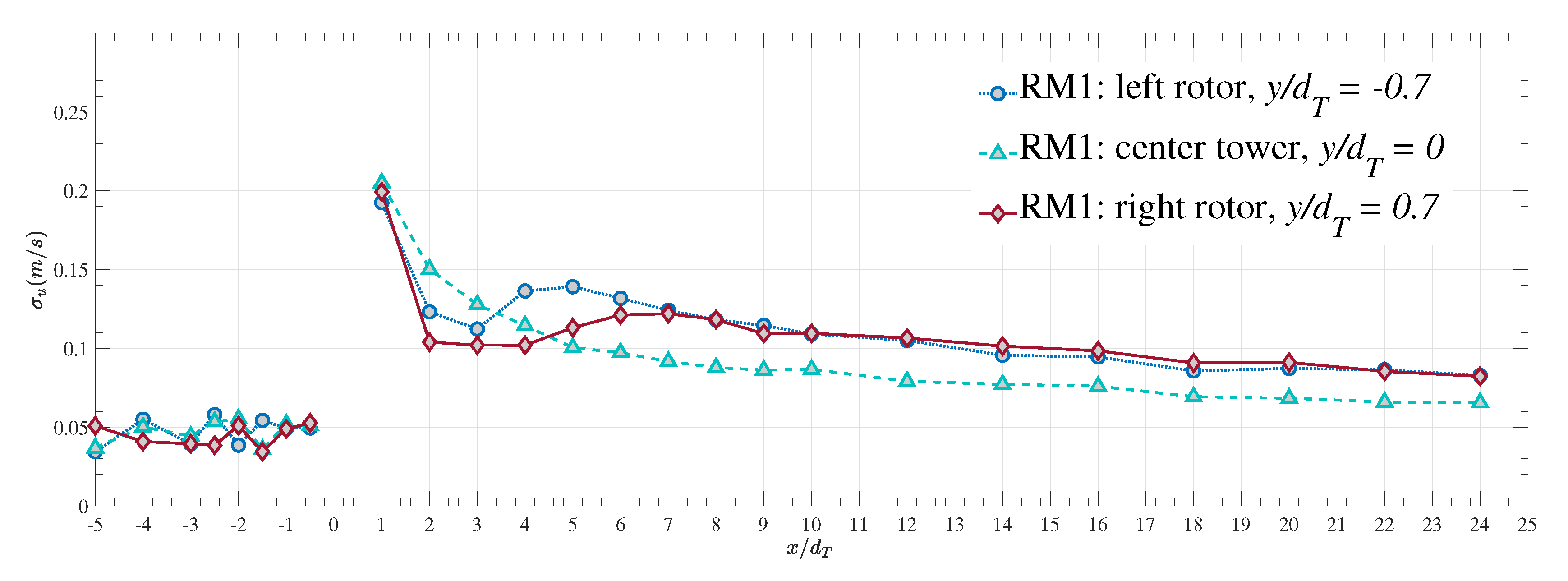
3.3. Wake Characteristics

Turbine wake velocity profiles were collected downstream of RM1 from 1 $d_T$ to 10 $d_T$ at 1 $d_T$ intervals. These data were collected along three vertically oriented ($xz$) planes aligned with each rotor center and the mid-plane ($y/d_T=$ 0) between the two rotors, as well as a horizontal ($xy$) plane aligned with the rotor hub height, $h_{hub}$. Contour plots of the streamwise velocity deficit, $u_{def}$, are illustrated in Figure 11. Additionally, normalized turbulent kinetic energy, $k/k_{\infty }$ are illustrated in Figure 12. The largest velocity deficit occurs in the near wake region at the center between the two rotors, immediately downstream of the center cylindrical vertical and horizontal support arms. The relatively high blockage ($\eta \approx$ 14.3%) forces flow acceleration to the outside of each rotor, as well as above and below each rotor, visible in Figure 11. The wake of each RM1 rotor quickly merges with the disturbance created by the center tower and forms a horizontally expansive wake that propagates far downstream and remains approximately the width of the full dual rotor RM1 assembly while diffusing and mixing with the surrounding flow. Elevated levels of turbulent kinetic energy are present in the downstream environment, particularly in the region aligned with the center support tower extending to approximately 2$d_T$. Additionally, the tip vortices originating from the blades introduce elevated regions of turbulent kinetic energy aligned with the top-tip and bottom-tip elevation of each rotor, evident in Figure 12.

It is common to report the velocity deficit at turbine hub height downstream of a turbine as a way to estimate the velocity recovery in the wake of a device. The RM1 rotors begin affecting inflow velocities up to approximately 2.5 $d_T$ to 3 $d_T$ upstream, at which point the flow decelerates by approximately 10% by the time it is one blade length upstream of the rotor energy extraction plane (Figure 13). The largest velocity deficit occurs in the wake of the center support tower ($u_{def}\approx$ 100%), where strong instabilities exist occurring in the form of von Kármán type vortices shed from the cylinder. The near-wake (≈ 1$d_T$) velocity deficit in the wake of each rotor is approximately 30% and increases up to about 3 $d_T$ to 4 $d_T$, at which point it begins to gradually recover. The relatively large blockage by the two rotors and center cylinder support tower generates a large wake that propagates far downstream. Hub height velocity measurements were collected up to 24 $d_T$, at which point the velocity deficit recovered to about 5% of the undisturbed approach flow in the wake of each rotor, while the center of the wake was still nearly 15% deficient. Similarly, neither streamwise turbulent fluctuations, $\sqrt{\overline{{u_i^{\prime }}^2}}$ (Figure 14), nor the streamwise turbulence intensity, $I_u$ (Figure 15), recovered to the undisturbed upstream equivalent values as far downstream as 24 $d_T$.

4. Discussion

4.1. Turbine Performance

Despite a slight difference in optimal performance between the RM1 left and right rotor, both rotors operated at maximum efficiency near $\lambda$ = 5.1 with $C_p\approx$ 0.43 to 0.48. The complexity of flow in the SAFL Main Channel facility and slight asymmetry in the approach flow may have been a factor in this observed difference. The resulting performance curves do show differences at optimal tip speed ratio, $\lambda$, of approximately 10%. Initial performance testing of the RM1 rotors revealed a $C_p$ vs. $\lambda$ curve similar to that shown in Figure 9. It was hypothesized that blade pitch on the left rotor was misaligned, thereby creating the decreased performance compared to the right rotor. To investigate this, performance measurements at several pitch angles for the left rotor were measured to verify that blades were fixed at the optimal angle. After collecting performance measurements at a turbine rotational speed of $\omega =$ 3.4 rps ($\lambda \approx$ 5.1), results indicated the optimal pitch angle was $\alpha =$ 0° for the initial performance tests completed.

The performance of this dual rotor turbine agreed well with other single rotor studies. In other observed physical model experiments, the optimal $C_p$ value was also observed to be in the $C_p$ = 0.4 to 0.5 range. For comparison, Lust et al. [10] observed optimal performance at approximately $\lambda$ = 6.5 with a corresponding $C_p$ = 0.41 for a single scaled model RM1 rotor in a large towing tank facility at the United States Naval Academy. Chamorro et al. [8] measured a $C_p$ = 0.45 at $\lambda$ = 5.8, Mycek et al. [47] observed a $C_p$ = 0.4 to 0.44 from $\lambda$ = 3.5 to 5.2, and most recently, Gaurier et al. [20] observed a broad peak in the $C_p$ vs. $\lambda$ curve, with efficiencies around $C_p=$ 0.41 between $\lambda =$ 3.5 and 5.8 and an increase in both performance and variability at higher turbulence levels (average $C_p\approx$ 0.46). Fontaine et al. [5] also documented a broad peak to the $C_p$ curve with values measured at $C_p$ > 0.4 from $\lambda$ = 2.9 to 6.9 with an optimal $C_p$ = 0.47. What is striking is the similarity in observed performance resulting from turbines of similar, yet slightly different geometries tested in tow tanks, water tunnels, and open-channel flumes. The consistency in these observations leads towards a deeper understanding of the performance capabilities of such CEC technologies. Furthermore, in many cases low $\lambda$ performance coefficients tracked similar values and were less susceptible to blade chord Reynolds number, agreeing with observations noted by [17,48,49]. At low $\lambda$ values, the local relative angle-of-attack along the length of the blade is generally high and typically beyond the stall angle for an airfoil (Figure 5b). Under these conditions, $C_L/C_D$ values are low and do not vary as Reynolds number changes, at least for the case of the NACA 4415 airfoil used for this model study. Conversely, at high $\lambda$ when local blade angles-of-attack may be negative, $C_L/C_D$ values are still low but show much larger variability as Reynolds number changes, perhaps causing the separation in rotor performance curves at higher tip speed ratios. Additionally, the low $\lambda$ side of the $C_p$ vs. $\lambda$ curve often exhibits a steep rise up to the optimal condition, with relatively flat peaks and gradual drop off in performance at higher $\lambda$, similar to that shown in Figure 9. In over-speed conditions (i.e., operating at a TSR greater than the optimal condition), the shape of performance curves showed greater variability and was more susceptible to increased turbulence levels [20].

It is important to note that while the performance of a dual-rotor turbine may not be balanced between the two rotors, the counter-rotating operation used in this study does not appear to degrade the individual performance of each rotor. Although performance characteristics of a single rotor operation were not directly measured in the present investigation, the observed power performance characteristics, including the best operating point, match those predicted using numerical models and other physical scaled model experiments of single rotors [50]. Asymmetric performance and loading, however, may intensify structural loads for devices that share a common support tower.

4.2. Wake Characteristics

Wake flow recovery in the present study exhibits most of the far-wake ($x/d_T\ge$ 5) characteristics observed for single rotor cases despite the added flow obstruction and turbulent mixing caused by the additional rotor, tower and cross-arm support wakes. For single rotor cases, the hub height centerline velocity deficit and turbulence intensity reduce exponentially from their maximum value, averaging 71% flow recovery and 20% turbulence intensity at $x/d_T=$ 5, to an average of 85% flow recovery and 13% turbulence intensity in the far-wake occurring at $x/d_T=$ 10 [31,33,34,35,36,47]. The wake deficit is persistent far downstream with an average of 92% flow recovery and 8% turbulence intensity in the far-wake occurring at $x/d_T=$ 20 [31,34,36]. Values for these parameters in the present dual rotor study are close to these average values with 70% (left rotor) and 68% (right rotor) flow recovery occurring at $x/d_T=$ 5, 89% (left rotor) and 84% (right rotor) at $x/d_T=$ 10, and 94% (left rotor) and 90% (right rotor) at $x/d_T=$ 20. Turbulence intensities were 19% (left rotor) and 16% (right rotor) at $x/d_T=$ 5, 12% for both rotors at and $x/d_T=$ 10, and 10% for both rotors at $x/d_T=$ 20. At $x/d_T=$ 25, the flow recovery for both rotors only slightly improves to approximately 95% with turbulence intensities just below 10%.

In the near wake ($x/d_T<$ 5), the observed values for velocity deficit and turbulence intensity for the present study deviate towards the the lower range of values reported for the near wake in single rotor studies at $x/d_T=$ 1, 2 and 3, but are still within the range of these values. The flow instability introduced by the center vertical support tower and horizontal support arms could increase mixing, thereby increasing wake mixing, accelerating recovery and decreasing recovery distance. We also hypothesize that the observed peak in velocity deficit occurring at $x/d_T$ = 3 rather than the more commonly reported monotonically decreasing wake deficit is due to the central support tower. The spacing of the two upstream rotors may cause flow acceleration between the two rotors. This accelerated flow then impinges on the central support tower and is diverted back towards the center of each rotor wake. This complex flow may result in increased immediate mixing in the near wake $x/d_T$ < 3; however, the measurements from these experiments do not provide enough insight into the exact cause of a velocity deficit peak occurring 3 $d_T$ downstream. A more streamlined support structure could be tested to study the impacts of the support structure on the power and near wake of this dual rotor turbine. Mycek et al. ([47]) reported a similar wake characteristic for a single rotor turbine, showing a slight increase in velocity deficit at $x/d_T$ = 4 when approach velocities had very low turbulence intensity ($I_u\approx$ 3%). The far-wake ($\ge x/d_T=$ 5) velocity deficit is similar between the single rotor and dual-rotor turbines (≈10%–20%). Not surprisingly, a consistent finding across many scaled model axial flow marine turbine studies is that the wake deficit is persistent, even far downstream of the rotor. Additional turbines downstream will have to operate in altered wake environments with enhanced turbulence and lower available power.

5. Conclusions

A 1:40 geometrically scaled model of the RM1, a dual-rotor axial-flow hydrokinetic turbine designed by the U.S. DOE for tidal environments, was tested in the St. Anthony Falls Laboratory Main Channel facility at the University of Minnesota. Detailed performance and upstream and wake velocity measurements were collected to assess the operation and interaction of RM1 with the surrounding environment resulting in an exceptionally robust dataset for numerical model validation and verification. Maximum $C_p$ was found to occur near $\lambda \approx$ 5.1 with values of $C_p=$ 0.48 for the right rotor and $C_p=$ 0.43 for the left rotor. Slight asymmetries in the approach flow environment may have caused the different rotor performance characteristics, but the root cause or causes were not determined. Performance was comparable to single rotor experiments, both in terms of efficiency, $C_P$, and tip-speed ratio, $\lambda$.

Detailed wake velocity measurements provide an indication of the turbulent wake environment, showing elevated levels of turbulent kinetic energy in the near wake environment, particularly resulting from the instabilities induced by the center support tower cylinder. Tip vortices also inject high turbulence levels that propagate up to approximately 4 $d_T$. Near-field wake recovery may have been enhanced due to the higher blockage of the RM1 experiments. Further investigations into the RM1 experimental data may reveal the mechanics of the near wake flow region and the influence of von Kármán frequencies shed from the center vertical and horizontal support arms have on the near wake structure of each rotor. What remains unknown is the effect of the proximity of the rotor plane to the horizontal support arm downstream of each rotor and the cross arm effect on turbine performance. This structural feature likely disrupts the near wake velocity and induce mixing more rapidly than other turbine configurations. Additional studies would benefit from studying performance and wake characteristics using variable cross-stream spacing, lag in turbine blade azimuth position, or controlling the relative rotational direction of each rotor, and how these variations in operational strategies impact blade stresses and complete structure loading.

The present study, like single rotor studies, shows that additional hydrokinetic turbine rotors downstream within an array or hydrokinetic turbine farm will operate in wake-altered flow environments, with degraded available power and increased turbulence levels, as it will likely be impractical and uneconomical to place additional turbines twenty or more diameters downstream. Implementing control optimization strategies and wake steering ([51]), therefore, may help maximize power plant efficiency.

References

1. Huckerby, J.; Jeffrey, H.; Sedgwick, J.; Jay, B.; Finlay, L. An International Vision for Ocean Energy—Version II; Ocean Energy Systems Implementing Agreement (OESIEA): Lisbon, Portugal, 2012. [Google Scholar]
2. Khan, M.; Bhuyan, G.; Iqbal, M.; Quaicoe, J. Hydrokinetic energy conversion systems and assessment of horizontal and vertical axis turbines for river and tidal applications: A technology status review. Appl. Energy 2009, 86, 1823–1835. [Google Scholar] [CrossRef]
3. Laws, N.D.; Epps, B.P. Hydrokinetic energy conversion: Technology, research, and outlook. Renew. Sustain. Energy Rev. 2016, 57, 1245–1259. [Google Scholar] [CrossRef] [Green Version]
4. Neary, V.S.; Lawson, M.; Previsic, M.; Copping, A.; Hallett, K.C.; LaBonte, A.; Rieks, J.; Murray, D. Methodology for Design and Economic Analysis of Marine Energy Conversion (MEC) Technologies; Technical Report; Sandia National Lab.(SNL-NM): Albuquerque, NM, USA, 2014. [Google Scholar]
5. Fontaine, A.; Straka, W.; Meyer, R.; Jonson, M.; Young, S.; Neary, V. Performance and wake flow characterization of a 1: 8.7-scale reference USDOE MHKF1 hydrokinetic turbine to establish a verification and validation test database. Renew. Energy 2020, 159, 451–467. [Google Scholar] [CrossRef]
6. Bahaj, A.; Molland, A.; Chaplin, J.; Batten, W. Power and thrust measurements of marine current turbines under various hydrodynamic flow conditions in a cavitation tunnel and a towing tank. Renew. Energy 2007, 32, 407–426. [Google Scholar] [CrossRef]
7. Maganga, F.; Germain, G.; King, J.; Pinon, G.; Rivoalen, E. Experimental characterisation of flow effects on marine current turbine behaviour and on its wake properties. IET Renew. Power Gener. 2010, 4, 498–509. [Google Scholar] [CrossRef] [Green Version]
8. Chamorro, L.P.; Hill, C.; Morton, S.; Ellis, C.; Arndt, R.E.A.; Sotiropoulos, F. On the interaction between a turbulent open channel flow and an axial-flow turbine. J. Fluid Mech. 2013, 716, 658–670. [Google Scholar] [CrossRef]
9. Luznik, L.; Flack, K.A.; Lust, E.E.; Taylor, K. The effect of surface waves on the performance characteristics of a model tidal turbine. Renew. Energy 2013, 58, 108–114. [Google Scholar] [CrossRef]
10. Lust, E.E.; Flack, K.A.; Luznik, L. Survey of the near wake of an axial-flow hydrokinetic turbine in quiescent conditions. Renew. Energy 2018, 129, 92–101. [Google Scholar] [CrossRef]
11. Walker, J.M.; Flack, K.A.; Lust, E.E.; Schultz, M.P.; Luznik, L. Experimental and numerical studies of blade roughness and fouling on marine current turbine performance. Renew. Energy 2014, 66, 257–267. [Google Scholar] [CrossRef]
12. Mycek, P.; Gaurier, B.; Germain, G.; Pinon, G.; Rivoalen, E. Experimental study of the turbulence intensity effects on marine current turbines behaviour. Part II: Two interacting turbines. Renew. Energy 2014, 68, 876–892. [Google Scholar] [CrossRef] [Green Version]
13. Chamorro, L.P.; Hill, C.; Neary, V.S.; Gunawan, B.; Arndt, R.E.A.; Sotiropoulos, F. Effects of energetic coherent motions on the power and wake of an axial-flow turbine. Phys. Fluids 2015, 27, 055104. [Google Scholar] [CrossRef]
14. Jing, F.m.; Ma, W.j.; Zhang, L.; Wang, S.q.; Wang, X.h. Experimental study of hydrodynamic performance of full-scale horizontal axis tidal current turbine. J. Hydrodyn. Ser. B 2017, 29, 109–117. [Google Scholar] [CrossRef]
15. Payne, G.S.; Stallard, T.; Martinez, R. Design and manufacture of a bed supported tidal turbine model for blade and shaft load measurement in turbulent flow and waves. Renew. Energy 2017, 107, 312–326. [Google Scholar] [CrossRef]
16. Barber, R.B.; Hill, C.S.; Babuska, P.F.; Wiebe, R.; Aliseda, A.; Motley, M.R. Flume-scale testing of an adaptive pitch marine hydrokinetic turbine. Compos. Struct. 2017, 168, 465–473. [Google Scholar] [CrossRef] [Green Version]
17. Ross, H.; Polagye, B. An experimental assessment of analytical blockage corrections for turbines. Renew. Energy 2020, 152, 1328–1341. [Google Scholar] [CrossRef] [Green Version]
18. Porter, K.E.; Ordonez-Sanchez, S.E.; Murray, R.E.; Allmark, M.; Johnstone, C.M.; O’Doherty, T.; Mason-Jones, A.; Doman, D.A.; Pegg, M.J. Flume testing of passively adaptive composite tidal turbine blades under combined wave and current loading. J. Fluids Struct. 2020, 93, 102825. [Google Scholar] [CrossRef]
19. Allmark, M.; Ellis, R.; Lloyd, C.; Ordonez-Sanchez, S.; Johannesen, K.; Byrne, C.; Johnstone, C.; O’Doherty, T.; Mason-Jones, A. The development, design and characterisation of a scale model Horizontal Axis Tidal Turbine for dynamic load quantification. Renew. Energy 2020, 156, 913–930. [Google Scholar] [CrossRef]
20. Gaurier, B.; Ikhennicheu, M.; Germain, G.; Druault, P. Experimental study of bathymetry generated turbulence on tidal turbine behaviour. Renew. Energy 2020, 156, 1158–1170. [Google Scholar] [CrossRef]
21. Bachant, P.; Wosnik, M.; Gunawan, B.; Neary, V.S. Experimental study of a reference model vertical-axis cross-flow turbine. PloS ONE 2016, 11, e0163799. [Google Scholar] [CrossRef] [Green Version]
22. Malki, R.; Masters, I.; Williams, A.J.; Croft, T.N. Planning tidal stream turbine array layouts using a coupled blade element momentum–computational fluid dynamics model. Renew. Energy 2014, 63, 46–54. [Google Scholar] [CrossRef] [Green Version]
23. Piano, M.; Robins, P.E.; Davies, A.G.; Neill, S.P. The Influence of Intra-Array Wake Dynamics on Depth-Averaged Kinetic Tidal Turbine Energy Extraction Simulations. Energies 2018, 11, 2852. [Google Scholar] [CrossRef] [Green Version]
24. Morandi, B.; Di Felice, F.; Costanzo, M.; Romano, G.; Dhomé, D.; Allo, J. Experimental investigation of the near wake of a horizontal axis tidal current turbine. Int. J. Mar. Energy 2016, 14, 229–247. [Google Scholar] [CrossRef]
25. Hill, C.; Musa, M.; Chamorro, L.P.; Ellis, C.; Guala, M. Local scour around a model hydrokinetic turbine in an erodible channel. J. Hydraul. Eng. 2014, 140, 04014037. [Google Scholar] [CrossRef]
26. Musa, M.; Hill, C.; Sotiropoulos, F.; Guala, M. Performance and resilience of hydrokinetic turbine arrays under large migrating fluvial bedforms. Nat. Energy 2018, 3, 839. [Google Scholar] [CrossRef]
27. Kadiri, M.; Ahmadian, R.; Bockelmann-Evans, B.; Rauen, W.; Falconer, R. A review of the potential water quality impacts of tidal renewable energy systems. Renew. Sustain. Energy Rev. 2012, 16, 329–341. [Google Scholar] [CrossRef]
28. Fraser, S.; Nikora, V.; Williamson, B.J.; Scott, B.E. Hydrodynamic impacts of a marine renewable energy installation on the benthic boundary layer in a tidal channel. Energy Procedia 2017, 125, 250–259. [Google Scholar] [CrossRef]
29. Li, X.; Li, M.; Amoudry, L.O.; Ramirez-Mendoza, R.; Thorne, P.D.; Song, Q.; Zheng, P.; Simmons, S.M.; Jordan, L.B.; McLelland, S.J. Three-dimensional modelling of suspended sediment transport in the far wake of tidal stream turbines. Renew. Energy 2020, 151, 956–965. [Google Scholar] [CrossRef]
30. Sparling, C.E.; Seitz, A.C.; Masden, E.; Smith, K. 2020 State of the Science Report-Chapter 3: Collision Risk for Animals around Turbines. Technical Report; Pacific Northwest National Lab.(PNNL): Richland, WA, USA, 2020. [Google Scholar]
31. Neary, V.; Gunawan, B.; Hill, C.; Chamorro, L. Near and far field flow disturbances induced by model hydrokinetic turbine: ADV and ADP comparison. Renew. Energy 2013, 60, 1–6. [Google Scholar] [CrossRef]
32. Stallard, T.; Feng, T.; Stansby, P. Experimental study of the mean wake of a tidal stream rotor in a shallow turbulent flow. J. Fluids Struct. 2015, 54, 235–246. [Google Scholar] [CrossRef]
33. Tedds, S.C.; Owen, I.; Poole, R.J. Near-wake characteristics of a model horizontal axis tidal stream turbine. Renew. Energy 2014, 63, 222–235. [Google Scholar] [CrossRef] [Green Version]
34. Stallard, T.; Collings, R.; Feng, T.; Whelan, J. Interactions between tidal turbine wakes: Experimental study of a group of three-bladed rotors. Philos. Trans. A. Math. Phys. Eng. Sci. 2013, 371. [Google Scholar] [CrossRef] [PubMed]
35. Chen, Y.; Lin, B.; Lin, J.; Wang, S. Experimental study of wake structure behind a horizontal axis tidal stream turbine. Appl. Energy 2017, 196, 82–96. [Google Scholar] [CrossRef]
36. Nuernberg, M.; Tao, L. Experimental study of wake characteristics in tidal turbine arrays. Renew. Energy 2018, 127, 168–181. [Google Scholar] [CrossRef] [Green Version]
37. Kang, S.; Yang, X.; Sotiropoulos, F. On the onset of wake meandering for an axial flow turbine in a turbulent open channel flow. J. Fluid Mech. 2014, 744, 376–403. [Google Scholar] [CrossRef]
38. Chawdhary, S.; Hill, C.; Yang, X.; Guala, M.; Corren, D.; Colby, J.; Sotiropoulos, F. Wake characteristics of a TriFrame of axial-flow hydrokinetic turbines. Renew. Energy 2017, 109, 332–345. [Google Scholar] [CrossRef] [Green Version]
39. Chawdhary, S.; Angelidis, D.; Colby, J.; Corren, D.; Shen, L.; Sotiropoulos, F. Multiresolution Large-Eddy Simulation of an Array of Hydrokinetic Turbines in a Field-Scale River: The Roosevelt Island Tidal Energy Project in New York City. Water Resour. Res. 2018, 54, 10–188. [Google Scholar] [CrossRef]
40. Aghsaee, P.; Markfort, C.D. Effects of flow depth variations on the wake recovery behind a horizontal-axis hydrokinetic in-stream turbine. Renew. Energy 2018, 125, 620–629. [Google Scholar] [CrossRef]
41. Neary, V.; Gunawan, B.; Sale, D. Turbulent inflow characteristics for hydrokinetic energy conversion in rivers. Renew. Sustain. Energy Rev. 2013, 26, 437–445. [Google Scholar] [CrossRef]
42. U.S. Department of Energy Tethys Engineering Reference Model Project. Available online: https://tethys-engineering.pnnl.gov/signature-projects/reference-model-project (accessed on 3 August 2020).
43. Douglas, C.; Harrison, G.; Chick, J. Life cycle assessment of the Seagen marine current turbine. Proc. Inst. Mech. Eng. Part J. Eng. Marit. Environ. 2008, 222, 1–12. [Google Scholar] [CrossRef] [Green Version]
44. Polagye, B.; Thomson, J. Tidal energy resource characterization: Methodology and field study in Admiralty Inlet, Puget Sound, WA (USA). Proc. Inst. Mech. Eng. Part J. Power Energy 2013, 227, 352–367. [Google Scholar] [CrossRef]
45. Goring, D.; Nikora, V. Despiking acoustic Doppler velocimeter data. J. Hydraulic Eng. 2002, 128, 117–126. [Google Scholar] [CrossRef] [Green Version]
46. Coleman, H.; Steele, W. Experimentation, Validation, and Uncertainty Analysis for Engineers, 3rd ed.; John Wiley & Sons, Inc.: New York, NY, USA, 2009. [Google Scholar]
47. Mycek, P.; Gaurier, B.; Germain, G.; Pinon, G.; Rivoalen, E. Experimental study of the turbulence intensity effects on marine current turbines behaviour. Part I: One single turbine. Renew. Energy 2014, 66, 729–746. [Google Scholar] [CrossRef] [Green Version]
48. Kolekar, N.; Banerjee, A. Performance characterization and placement of a marine hydrokinetic turbine in a tidal channel under boundary proximity and blockage effects. Appl. Energy 2015, 148, 121–133. [Google Scholar] [CrossRef]
49. Kinsey, T.; Dumas, G. Impact of channel blockage on the performance of axial and cross-flow hydrokinetic turbines. Renew. Energy 2017, 103, 239–254. [Google Scholar] [CrossRef]
50. Michelen, C.; Neary, V.S.; Murray, J.; Barone, M.F. CACTUS Open Source Code for Hydrokinetic Turbine Design and Analysis: Model Performance Evaluation and Public Dissemination as Open Source Design Tool; Technical Report; Sandia National Lab. (SNL-NM): Albuquerque, NM, USA, 2014. [Google Scholar]
51. Musa, M.; Ravanelli, G.; Bertoldi, W.; Guala, M. Hydrokinetic Turbines in Yawed Conditions: Toward Synergistic Fluvial Installations. J. Hydraul. Eng. 2020, 146, 04020019. [Google Scholar] [CrossRef]
Figure 1. (a) Photo of RM1 installed in the SAFL Main Channel Facility. (b) CAD image showing internal instrumentation setup for data acquisition of turbine performance.
Energies 13 05145 g001
Figure 2. Detailed dimensions of the 1:40 scale RM1 turbine tested at SAFL (a) looking from upstream towards the turbine and (b) side view of the rotor and nacelle. CAD files for RM1 are available through the Tethys Engineering Signature Project website.
Energies 13 05145 g002
Figure 3. Experimental setup and ADV sampling location schematic of RM1 testing in the SAFL Main Channel facility.
Energies 13 05145 g003
Figure 4. Comparison between full-scale blade geometric characteristics for the original RM1 blade design (NACA-63(4)-24) and the modified design (NACA-4415) for lower Reynolds number testing at SAFL.
Energies 13 05145 g004
Figure 5. Model of chord length Reynolds number (a) and local relative angle-of-attack (b) for the RM1 model-scale NACA 4415 blades. Vertical dashed white lines bound the region of measured optimal performance.
Energies 13 05145 g005
Figure 6. Ratio between simulated model and field scale (a) lift and (b) drag coefficients for a range of tip speed ratios. Red circles identify results near measured optimal performance for the RM1 model-scale turbine.
Energies 13 05145 g006
Figure 7. Inflow vertical profile characteristics in the center of the channel at 3 d T upstream of RM1: mean streamwise velocity, u ¯ (left), streamwise velocity root-mean squared, σ u = u i 2 ¯ (center), and streamwise turbulence intensity, I u (right). Area between dashed lines −0.25 m Z 0.25 m indicates RM1 rotor energy extraction plane. Mean water surface elevation (WSE) is indicated by dashed line at Z = 0.5 m. Turbine hub height, h h u b , is located at z = 0 m.
Energies 13 05145 g007
Figure 8. Inflow horizontal profile characteristics at hub height, h h u b , from 3 d T upstream of RM1: mean streamwise velocity, u ¯ (top), streamwise velocity root-mean squared, σ u = u i 2 ¯ (center), and streamwise turbulence intensity, I u (bottom). Y-axis distance shows full channel width, b = 2.75 m.
Energies 13 05145 g008
Figure 9. Calculated C p vs. λ (coefficient of power vs. tip-speed ratio) for the left (blue) and right (red) RM1 rotors. Vertical error bars represent mean C p value measurement uncertainty. Maximum C p occurs near λ 5.1 (right rotor C p = 0.48; left rotor C p = 0.43). Results have not been corrected for channel blockage; therefore, maximum C p may slightly decrease after blockage corrections have been applied.
Energies 13 05145 g009
Figure 10. Instantaneous torque (light gray dots) measurements, τ i vs. instantaneous rotor blade angular position, θ i ( ° ) . Solid black line illustrates mean torque value, τ ¯ vs. rotor blade angular position, θ ( ° ) . Measurements collected from right rotor while turbine was operating at ω = 3.4 rps ( λ 5.1). RM1 blades are offset 180° on each rotor but were counter-rotating in symmetry.
Energies 13 05145 g010
Figure 11. Velocity deficit horizontal ( x y ) and vertical ( x z ) plane contours upstream and downstream of RM1 in the SAFL Main Channel. Horizontal plane y-axis, y / d T , shows full channel width ( b = 2.75 m). Vertical planes y-axis, z / d T , shows full water depth during the experiment ( h = 1.0 m). Horizontal and vertical dotted black lines indicate actual ADV measurement locations. ADV vertical point spacing Δ z = 0.025 m ( z / d T = 0.05). Horizontal spacing varied. Measurements collected at λ 5.1 ( ω = 3.4 rps). Flow is left to right.
Energies 13 05145 g011
Figure 12. Normalized turbulent kinetic energy, k / k , horizontal ( x y ) and vertical ( x z ) plane contours upstream and downstream of RM1 in the SAFL Main Channel. Horizontal plane y-axis, y / d T , shows full channel width ( b = 2.75 m). Vertical plane y-axis, z / d T , shows full water depth during the experiment ( h = 1.0 m). Horizontal and vertical dotted black lines indicate actual ADV measurement locations. ADV vertical point spacing Δ z = 0.025 m ( z / d T = 0.05). Horizontal spacing varied. Measurements collected at λ 5.1 ( ω = 3.4 rps). Flow is left to right.
Energies 13 05145 g012
Figure 13. Hub height velocity deficit. RM1 rotors located at x / d T = 0. Measurements collected at λ 5.1 ( ω = 3.4 rps).
Energies 13 05145 g013
Figure 14. Hub height streamwise root-mean squared ( σ u = u 2 ¯ ). RM1 rotors located at x / d T = 0. Measurements collected at λ 5.1 ( ω = 3.4 rps).
Energies 13 05145 g014
Figure 15. Hub height streamwise turbulence intensity, I u . RM1 rotors located at x / d T = 0. Measurements collected at λ 5.1 ( ω = 3.4 rps).
Energies 13 05145 g015