Article

Fault Prognostics for Photovoltaic Inverter Based on Fast Clustering Algorithm and Gaussian Mixture Model

1
Department of Materials Science and Engineering, University of Science and Technology of China, Hefei 230026, China
2
State Grid Electric Power Research Institute, Nanjing 211106, China
3
Department of Energy and Power Engineering, Tsinghua University, Beijing 100084, China
*
Author to whom correspondence should be addressed.
Energies 2020, 13(18), 4901; https://doi.org/10.3390/en13184901
Submission received: 12 July 2020 / Revised: 13 September 2020 / Accepted: 17 September 2020 / Published: 18 September 2020
(This article belongs to the Section A2: Solar Energy and Photovoltaic Systems)

Abstract

:
The fault prognostics of the photovoltaic (PV) power generation system is expected to be a significant challenge as more and more PV systems with increasingly large capacities continue to come into existence. The PV inverter is the core component of the PV system, and it is essential to develop approaches that accurately predict the occurrence of inverter faults to ensure the PV system’s safety. This paper proposes a fault prognostics method which makes full use of the similarities between inverter clusters. First, a feature space was constructed using the t-distributed stochastic neighbor embedding (t-SNE) algorithm. Then, the fast clustering algorithm was used to search the center inverter of each sampling time from the feature space. The status of the center inverter was adopted to establish the health baseline. Finally, the Gaussian mixture model was established with two data clusters based on the central inverter and the inverter to be predicted. The divergence of the two clusters could be used to predict the inverter’s fault. The performance of the proposed method was evaluated with real PV monitoring data. The experimental results showed that the proposed method successfully predicted the occurrence of an inverter fault 3 months in advance.

1. Introduction

With increasingly serious global environmental pollution and energy shortage, solar energy, as a renewable and pollution-free new energy source, has received extensive attention in recent years [1,2]. The photovoltaic (PV) power generation system is an important device which converts solar energy into electrical energy [3]. The PV array generates a direct current through the photoelectric effect, and then the inverter is responsible for converting the direct current into a usable alternating current that finally is merged into the power grid or directly provided to the load [4,5]. As a key component of the PV power generation system, the PV inverter’s status and performance directly affect the operation safety of the system. At present, the maintenance of the PV power generation system is usually serviced after an accident or maintained periodically [6,7,8]. Sudden failure of the PV inverter will lead directly to a reduction in system power generation and a substantial increase in maintenance costs [9]. Therefore, with the help of fault prognostics technology, it is particularly important to transform “timely maintenance” into “intelligent maintenance” for the PV inverter.
Scholars have performed some meaningful studies on PV system fault diagnosis and prognostics. Garoudja et al. proposed a model-based fault detection method for early detection of shading of PV modules and faults on the direct current side of PV systems. This method mainly used the extended capacity of an exponentially weighted moving average control chart to detect incipient changes in a PV system [10]. Fazai et al. proposed an approach that adopted the Gaussian process regression as a framework, and a generalized likelihood ratio test chart was applied to detect PV system faults [11]. Yi et al. investigated line-to-line fault detection in the PV system using multi-resolution signal decomposition and two-stage support vector machine classifiers. The training data were the total voltage and current from PV arrays [12]. These studies mainly used different data processing methods to extract the slight differences between the initial state of the equipment and the current state and then used them to identify system failures. However, for a certain device, its initial state is easily affected by environmental factors. Ameur et al. investigated and compared the impact of different factors on the performance of different PV types [13]. Basnet et al. found that certain faulty states in a PV system closely resemble a normal state, especially during the winter season. Thus, a normal fault detection model can falsely characterize a well-operating PV system as a faulty state and vice versa [14]. Therefore, environmental factors directly affect the accuracy of the established initial state or health baseline.
Huang et al. investigated the degradation process of photovoltaic modules, establishing a circuit-based model to describe the relationship between environmental factors and the aging process of photovoltaic modules. The results showed that the degradation process can be very complicated depending on the degradation patterns of aging [15]. Chin et al. investigated a hybrid method by combining the analytical method with the differential evolution optimization technique. Then, an accurate computational model was proposed for the two-diode model of the PV module [16]. Zegaoui et al. introduced a universal transistor-based hardware simulator of a photovoltaic simulator. This simulator was dedicated to simulations and performing various tests of a complete PV system under various environmental conditions [17]. Although the above-mentioned photovoltaic system simulation based on algorithms or hardware simulated the equipment performance degradation process under different environmental factors, on-site simulation and debugging of algorithms or hardware pose a huge challenge for the maintenance engineers, which leads to poor applicability in the field.
In a PV system, PV inverters are usually installed and operated under similar conditions. To reduce the impact of environmental factors, we can make full use of the similarities between inverter clusters when the equipment health baseline is established. The core idea of this paper is to utilize the fast clustering algorithm to search the center inverter of each sampling time in the feature space and to construct the health baseline of the cluster directly using the initial status of the equipment to build the health baseline.
Figure 1 shows the main technical framework of this paper. The acquired operating data of the PV inverter are high-dimensional data. High-dimensional data are difficult to observe directly and will affect the calculation efficiency, so it is necessary to reduce the dimensionality of high-dimensional data to a low-dimensional space for observation and calculation. t-distributed stochastic neighbor embedding (t-SNE) is a data preprocessing method for dimensionality reduction which has been widely used in wind farm monitoring data and the equipment vibration signal preprocessing field. Gu et al. proposed a data preprocessing algorithm based on the t-SNE algorithm to reduce the dimensionality of the numerical weather prediction data related to wind farm operation. The results showed that the prediction accuracy of the wind farm operation had been improved by combining the preprocessed numerical weather prediction data [18]. Zheng et al. proposed a fault diagnosis method for rolling bearing by combining multiscale fuzzy entropy with t-SNE. As a feature dimension reduction method, t-SNE was utilized to obtain the low-dimensional manifold features of rolling bearing [19]. t-SNE firstly uses the conditional probability distribution to express the similarity between points in high-dimensional space. In the low-dimensional space, the probability distribution of these points is constructed by t-distribution. Then, the gradient of the Kullback–Leibler divergence between two probability distributions is deduced to pursue the result that the two probability distributions are as similar as possible. In this way, a point distribution similar to the point distribution in the high-dimensional space is constructed in the low-dimensional space [20,21,22]. Here, t-SNE is applied to reduce the monitoring data dimensionality and construct a two-dimensional feature space.
To search the center inverter from the PV inverter cluster in two-dimensional feature space, a fast clustering algorithm published in Science in 2014 was adopted. This algorithm was based on the idea that centers are surrounded by neighbors with lower densities and are characterized by large distances from points with higher densities [23]. The idea of the fast clustering algorithm is novel and the calculation is concise. It performs better than the traditional clustering algorithm on various datasets [24,25]. Thus, the fast clustering algorithm is used to search the center inverter from inverter cluster. The Gaussian mixture model plays an important role in data cluster analysis and has been applied in fault diagnosis and uncertainty analysis on wind turbines [26,27,28]. Consequently, the Gaussian mixture model is applied to compare the feature distributions between the inverter to be predicted and the center inverter. To quantify the difference of different inverter feature distributions in the Gaussian mixture model, Jensen–Shannon divergence (JSD) is used to measure the difference in Gaussian distributions and, finally, the overlap rate, which can be used as a health indicator, is established and applied in prognostics.
Our work in this paper mainly focuses on three issues that have not been touched upon in earlier work. Firstly, a method for establishing the health baseline based on the inverter group is proposed. Usually, the health baseline is only based on the initial data of a single piece of equipment. Since the parameters of the PV inverter are easily affected by the season, sunshine, and other environmental factors, the health baseline is inevitably strongly interfered with by these factors. For the health baseline based on the inverter group, since the inverter to be predicted and the central inverter are in the same working condition all the time, the influence of environmental factors is effectively reduced.
Secondly, a quantitative indicator of health status is proposed. A Gaussian mixture model is constructed based on the feature distribution, and the difference between different feature distributions is quantified through JSD, and then the health indicator is calculated, which successfully realizes the quantification of the inverter health status.
Thirdly, the fault prognostics of the inverter are realized. This method makes full use of the information of the inverter group, refers to the health status of the entire inverter group, and sets the early warning line, so as to successfully realize the PV inverter fault prognostics.
The remaining general outline of this paper is as follows. In Section 2, the PV inverter and time-series monitoring data are presented. The main theories of the proposed fault prognostics method are detailed in Section 3. The experimental performance of the proposed method is evaluated with real PV monitoring data in Section 4. Finally, Section 5 presents the conclusions from this paper.

2. PV Inverter Condition Monitoring
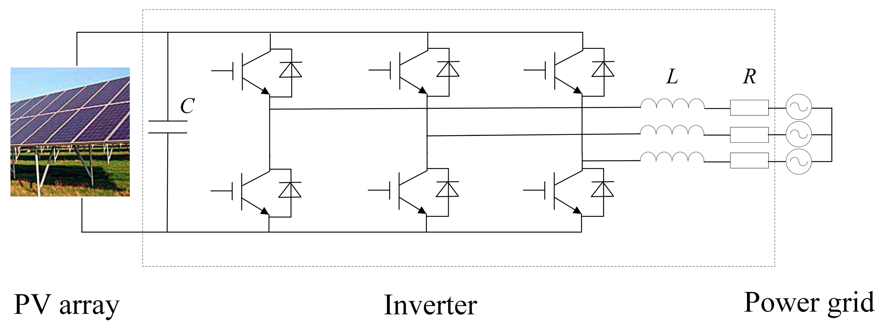
2.1. PV Inverter

Figure 2 shows the main circuit of the PV power generation system. As the key component of connecting the PV array and power grid, the PV inverter is mainly responsible for two tasks: controlling the maximum power point of the PV array and injecting sinusoidal current into the power grid.
Common faults of the PV power generation system are shown in Table 1. When the common faults described in Table 1 occur, especially the faults caused by damage to inverter components, the PV power generation system enters the shutdown state and stops generating power. Then, the maintenance personnel conduct on-site troubleshooting and maintenance. Therefore, with the help of a condition monitoring system and data processing technology, accurate fault prognostics of the PV inverter could be achieved, which would be particularly significant for maintenance personnel.

2.2. Time-Series Monitoring Data

The dataset adopted in this paper corresponds to a set of 20-min resolution readings from a distributed PV power generation system. This system monitors the operating parameters of 9 PV inverters established on the top of a building located in an industrial park in Nanjing city, from 2017 to 2018. The inverter type is a string inverter and the model no. is NS46K. The rated output power is 46 kw and the maximum output current is 55.5 A. These nine inverters are under the same operating conditions.
We formulated the fault prognostics problem for the PV inverter as a statistical parameter estimation problem. The 20-min resolution readings can be treated as time-series data, with the frequency of f readings per day (f = 36, since readings from 6 a.m. to 6 p.m. were monitored in this study). In each reading, each PV inverter collected 25 signals, including output power, three-phase voltage, three-phase current, Insulated Gate Bipolar Transistor (IGBT) temperature, PV DC current, PV DC voltage, etc. Let ym(td,i) denote the ith reading matrix of the mth PV inverter for day d, then
y m ( t d , i ) = [ a 1 , a 2 , , a n ] ,
where an represents the nth signal of the mth PV inverter.
For the mth PV inverter, the sequence matrix of readings for day d can be expressed as
D m ( d ) = [ y m ( t d , 1 ) , y m ( t d , 2 ) , , y m ( t d , f ) ] T ,
where T is the matrix transpose symbol.
The daily sampled readings during k days can be batched into a data bundle matrix as
Y m ( d ) = [ D m ( d ) , D m ( d + 1 ) , , D m ( d + k 1 ) ] .
The data bundle Ym(d) is later adopted as input for the PV inverter fault prognostics method. The method focuses on comparing the differences between data bundles of different PV inverters. Figure 3 shows the formulation and utilization of the monitoring data. Although sophisticated sensors of the condition monitoring system are able to deliver data about the inverter’s status, the problem is that these data are of little or no practical use. To enhance the visibility of the data, the data processing technology is applied to project these data into a low-dimensional visible space.

3. Fault Prognostics Method

3.1. t-SNE

As a data processing technology, t-SNE is mainly applied for data dimension reduction or feature extraction, especially suitable for the reduction of high-dimensional data to two or three dimensions for easy visualization [29,30]. t-SNE adopts the conditional probabilities to describe the similarities between data points. The set of data points X = {x1, x2, …, xn} is a high-dimensional dataset. xi and xj are any two data points in the set X. The conditional probability pj|i represents the similarity of data point xj to data point xi, shown as
p j | i = exp ( x i x j 2 / 2 σ i 2 ) k i exp ( x i x k 2 / 2 σ i 2 ) ,
where σi is the variance of the Gaussian distribution centered on data point xi.
We use yi and yj representing the counterparts of the data points xi and xj in low-dimensional space. The variance of the low-dimensional Gaussian distribution is set as 1 / 2 . Hence, the similarity of data point yj to data point yi is expressed as
q j | i = exp ( y i y j 2 ) k i exp ( y i y k 2 ) .
In symmetric SNE, the pairwise similarities in low-dimensional space are
q i j = exp ( y i y j 2 ) k l exp ( y k y l 2 ) .
In high-dimensional space, the pairwise similarities are
p i j = exp ( x i x j 2 / 2 σ 2 ) k l exp ( x k x l 2 / 2 σ 2 ) .
The sum of the Kullback–Leibler divergence between joint probability distributions of high-dimensional space and low-dimensional space is
C = i j p i j ln p i j q i j .
The gradient of symmetric SNE is defined as
δ C δ y i = 4 j ( p i j q i j ) ( y i y j ) .
Thus, the t-SNE can recover the low-dimensional manifold structure of the data from the high-dimensional space, so as to effectively reduce the data dimension.

3.2. Fast Clustering Algorithm

In a PV inverter group maintained regularly, all PV inverters work in a similar environment and most of them are in a normal working state at any time. Therefore, the technical route for health baseline selection involves taking the state of equipment located in the feature distribution center as the health baseline from the feature distribution of the PV inverter group. To search the center of the feature distribution effectively, we applied a novel fast clustering algorithm. The fast clustering algorithm assumes that centers own higher local densities than the points surrounding them [31]. Meanwhile, the centers are at a relatively long distance from the points with higher local densities. To calculate the local density, two methods, including Gaussian kernel and cut-off kernel, can be used. With Gaussian kernel, the local density ρi of data point i is defined as
ρ i = j e ( d i j d c ) 2 ,
where dij represents the distance between data point i and data point j; dc represents the cut-off distance.
With cut-off kernel, the local density ρi can be expressed as
ρ i = j χ ( d i j d c ) ,
χ ( x ) = { 0 , x 0 1 , x < 0 .
From Equations (10) to (12), it is clear that the local density ρi implies the number of data points surrounding the data point i compared with dc.
Then, the distance δi is
δ i = { min j I ( d i j ) , I Ø max j I ( d i j ) , I = Ø ,
where I is the set that ρi is less than ρj.
Equation (13) shows that the distance δi denotes the minimum distance between the data point i and data points with a higher density.
Next, we calculate the weight of each data point. The weight γi of data point i is defined as
γ i = ρ i δ i .
It is obvious that center points are data points with larger weights. We use qi to represent the index number of local density ρi sorted in descending order. Then, a sequence nqi can be defined as
n q i = arg min d q i q j ( q j ) , i 2   &   i > j .
The sequence nqi represents the index number of the point closest to data point i and with larger local density than data point i.
Finally, the points can be categorized as
c q i = c n q i ,
where c denotes the label of the center points.

3.3. Gaussian Mixture Model

The Gaussian mixture model plays an important role in data cluster analysis. Usually, the clustering algorithm’s performance depends on whether the clustering results contain well-separated data clusters—in other words, whether the data clusters of the Gaussian mixture model overlap with each other. In this paper, we construct the Gaussian mixture model between the feature distribution of the PV inverter to be evaluated and the feature distribution center of the PV inverter group. Then, the clusters’ divergence of the Gaussian mixture model is used to evaluate the PV inverter’s health state.
A set of k data clusters can be formed as Z = {Z1, Z2, …, Zk}, where Zi represents a vector of d dimensions. In the finite Gaussian mixture model, each Zi can be viewed as a hump from a mixture model of k Gaussian distributions. The probabilistic density function is expressed as
{ p ( Z ) = i = 1 k α i Z i ( μ i , i ) Z R d i = 1 k α i = 1          ( 0 α i 1 ) ,
where (μii) represent the mean and the covariance matrix for Zi. Zi is the ith data cluster, defined as
Z i = 1 ( 2 π ) d / 2 | i | 1 / 2 e x p ( 1 2 ( Z μ i ) T Σ i 1 ( Z μ i ) ) .
A schematic diagram of an inverter’s feature distribution is shown in Figure 4. The left part of Figure 4 shows the feature space composed of feature 1 and feature 2. The health baseline is established by the central inverter feature distribution of the PV inverter group. The health baseline is marked as Z1, and the mean and the covariance matrix are (μ11). For any inverter in the PV inverter group, the feature distribution is marked as Z2, and the mean and the covariance matrix are (μ22). With the performance degradation, the feature distribution of the inverter would change; that is, the mean and the variance would change. In the feature space, the feature distribution of the inverter gradually deviates from the health baseline. The right part of Figure 4 shows the corresponding Gaussian mixture model. According to the mean and the covariance matrix (μ11), the health baseline Z1, one hump of the Gaussian mixture model, can be constructed. Then, the feature distribution Z2 of the inverter to be evaluated, another hump of the Gaussian mixture model, can be formed. As a result of the differences in mean and variance matrix between Z1 and Z2, the height and width of these two humps are different. The divergence of these two humps can be used to represent the performance degradation of the inverter to be evaluated.
In this paper, our research of the divergence of the Gaussian mixture model follows an approach that is practical for real applications. Our study is restrained to the divergence of two clusters, and the divergence phenomenon of three or more clusters can be dealt with by our method in a pair-wise comparison.

3.4. Fault Prognostics

As mentioned above, the central inverter feature distribution of the PV inverter group constructs the health baseline, which is one hump Z1 of the Gaussian mixture model. The feature distribution of the inverter to be evaluated forms another hump Z2. Therefore, JSD is introduced to effectively measure the divergence of two humps of the Gaussian mixture model [32,33].
JSD is proposed based on information entropy theory. The probability of the discrete random variable X is defined as P = {p1, p2, …, pn}. Then, the information entropy of the variable X is
H ( X ) = p i ln ( p i ) .
The information entropy of the variable Y is
H ( Y ) = q i ln ( q i ) ,
where Q = {q1, q2, …, qn} is the probability of the variable Y.
Then, the Kullback–Leibler divergence between the probability distribution P and Q is defined as follows:
C K L ( P , Q ) = p i ln p i q i .
The E(P,Q) are constructed as follows:
I ( P , Q ) = C K L ( P , 1 2 P + 1 2 Q ) ,
E ( P , Q ) = I ( P , Q ) + I ( Q , P ) .
According to the formula of information entropy, we can get
E ( P , Q ) = 2 H ( P + Q 2 ) H ( P ) H ( Q ) .
The JSD DJS(P,Q) calculation formula for probability P and Q is
D J S ( P , Q ) = H ( π 1 P + π 2 Q ) π 1 H ( P ) π 2 H ( Q ) ,
where π1 and π2 are weights of probability P and Q, respectively.
DJS(P,Q) is close to zero when probability P and Q are similar.
Analogously, we can extend JSD to the Gaussian mixture model. Z1 = (μ11) and Z2 = (μ22). Then, the JSD approximation is as follows:
D J S ( Z 1 , Z 2 ) = H ( π 1 Z 1 + π 2 Z 2 ) π 1 H ( Z 1 ) π 2 H ( Z 2 ) .
Let π1 and π2 be equal to 1/2, respectively. Then,
D J S ( Z 1 , Z 2 ) = 1 2 ( C K L ( Z 1 , M ) + C K L ( Z 2 , M ) ) .
M is the midpoint distribution, which can be calculated as
M ( x i ) = 1 2 Z 1 ( x i ) + 1 2 Z 2 ( x i ) ,
where xi represent the data sampled from Z1 or Z2.
C K L ( Z 1 , M ) = Z 1 ( x ) ln ( Z 1 ( x ) M ( x ) ) d x
C K L ( Z 2 , M ) = Z 2 ( x ) ln ( Z 2 ( x ) M ( x ) ) d x
The Monte Carlo approximations of these are
C K L a p p r o ( Z 1 , M ) = 1 n i = 1 n ln ( Z 1 ( x i ) M ( x i ) ) ,
C K L a p p r o ( Z 2 , M ) = 1 n i = 1 n ln ( Z 2 ( x i ) M ( x i ) ) .
Combining Equations (27), (31), (32), the expression of the JSD approximation is
D J S ( Z 1 , Z 2 ) = 1 2 ( C K L a p p r o ( Z 1 , M ) + C K L a p p r o ( Z 2 , M ) ) .
The overlap rate of the Z1 and Z2 multivariate Gaussian distributions is defined as
O r a t e ( Z 1 , Z 2 ) = 1 D J S ( Z 1 , Z 2 ) .
Orate(Z1, Z2) is close to 1, when the Z1 and Z2 multivariate Gaussian distributions are similar.
In short, the JSD is used to evaluate the divergence of two humps. Then, the overlap rate is applied to express the similarity of two humps and adopted as the health indicator.
Figure 5 shows the flow chart of fault prognostics. JSD is adopted to measure the divergence of two humps of the Gaussian mixture model. Then, the overlap rate is deduced and treated as a health indicator. By setting a reasonable early warning line, an early warning is given when the health indicator value crosses the early warning line. Therefore, the PV inverter fault prognostics can be realized.
In conclusion, the data processing process of the proposed fault prognostics approach is as follows: the operating parameters of 9 PV inverters are monitored. Each PV inverter collects 25 parameters. To reduce the data dimension, the t-SNE method is used to extract two features from 25 monitoring parameters. Then, a feature space composed of two extracted features can be formed. In the feature space, the fast clustering algorithm is applied to search the central inverter feature distribution of the PV inverter group. Therefore, the health baseline can be established and treated as one hump of the Gaussian mixture model. The feature distribution of the inverter to be evaluated forms another hump. Finally, the overlap rate is calculated to express the similarity of the two humps and is adopted as the health indicator.

4. Experimental Results and Discussion

4.1. Features Extraction

Among all PV monitoring parameters, the output power of the PV inverter is very important. Figure 6 shows the normalized output power of an inverter throughout 1 year. Meanwhile, the weekly maximum of the output power is also plotted to observe the change trend of the output power. The calculation formula for normalized output power P′ is
P = P P min P max P min ,
where P is the output power, and Pmax and Pmin represent the maximum and minimum output power, respectively.
It can be seen from Figure 6 that the maximum output power of the PV inverter in August, September, and October is lower than the values in other months. There is plenty of sunshine in August, September, and October. However, the air temperature, humidity, and rainfall are relatively high and frequent in summer and autumn. These environmental factors have a great impact on PV inverter power generation. In August, September, and October, the high temperature affects the PV module, which in turn affects the PV inverter power generation. The peak temperature coefficient of the PV module is approximately −0.5%/°C; that is, the higher the temperature, the lower the PV inverter power generation. On the basis of the above analysis, it is clear that the output power change in the PV inverter does not represent a single trend, and there is no direct positive or negative correlation between the PV inverter’s monitoring parameters and the performance degradation trend.
For easy visualization and data dimension reduction, the t-SNE method is used for extracting two features from 25 monitoring parameters of a PV inverter. t-SNE is a nonlinear dimensionality reduction method. The probability distribution of pairwise similarities in low-dimensional space is shown in Equation (6). The probability distribution of pairwise similarities in high-dimensional space is shown in Equation (7). The sum of the Kullback–Leibler divergence between probability distributions of high-dimensional space and low-dimensional space is shown in Equation (8). Then, the gradient of the Kullback–Leibler divergence between two probability distributions is deduced to pursue the result that the two probability distributions are as similar as possible. In this way, a point distribution similar to the point distribution in the high-dimensional space is constructed in the low-dimensional space [20,21,22]. Two extracted features do not directly select two parameters from the 25 monitoring parameters but are the result of nonlinear mapping of the 25 monitoring parameters. Therefore, this process is “features extraction”.
We divided the monitoring time of the PV inverter into three periods. The first period is from May 2017 to July 2017, the second period is from August 2017 to December 2017, and the third period is from January 2018 to April 2018. Figure 7 shows the probability distributions of two extracted features in different periods. Observing the feature probability distribution, Figure 7 shows that the probability distribution trend does not correlate with performance degradation. In short, the monitoring data of PV inverters is affected by environmental factors such as temperature, humidity, rainfall, etc. In addition, it is difficult to show a clear correlation with performance degradation with the extracted features. The usual method of taking the initial status as the health baseline is not applicable for PV inverter fault prognostics. Therefore, we select the status of the inverter located in the feature distribution center as the health baseline from the PV inverter group.

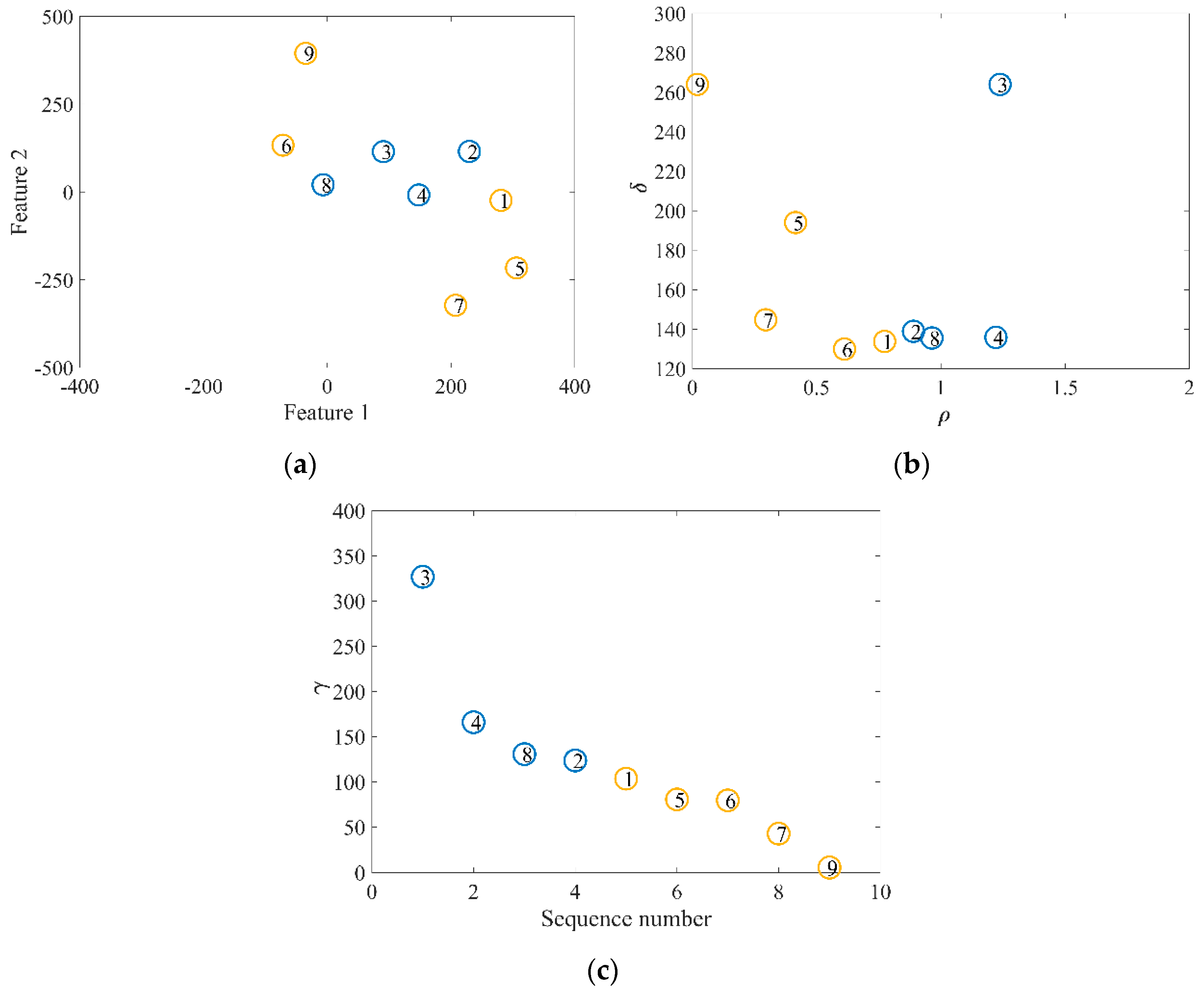
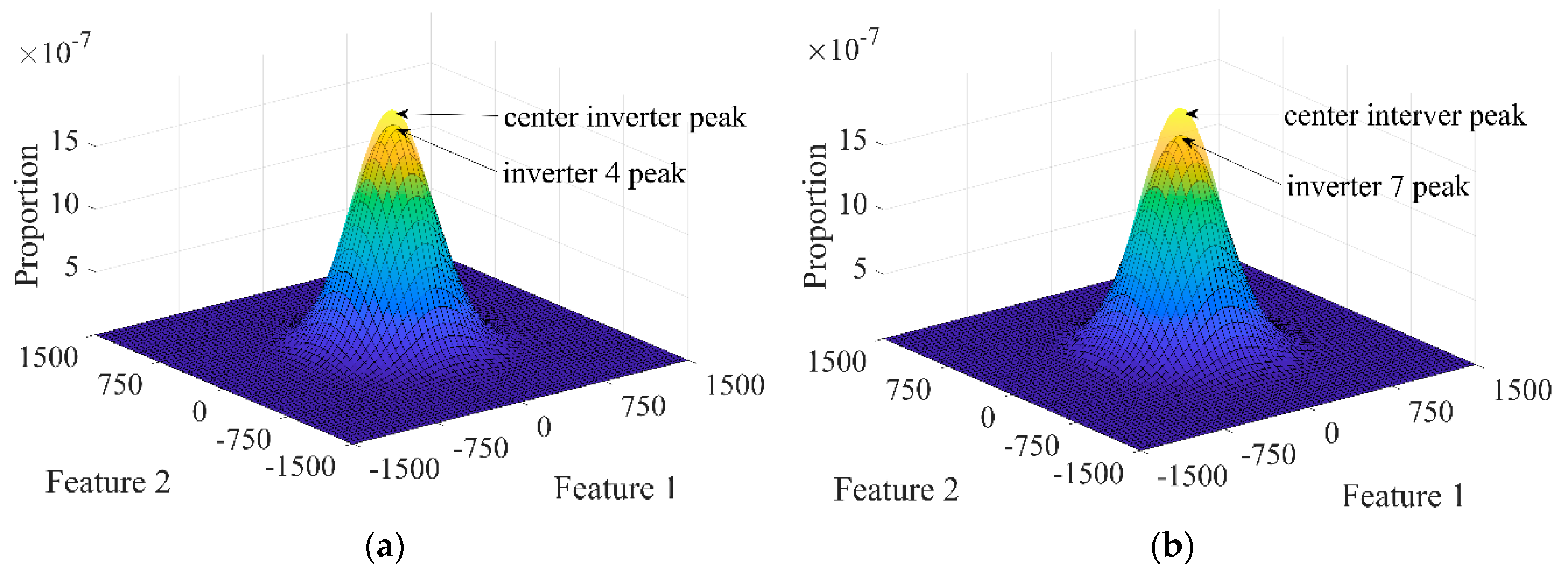
4.2. Center Inverter Search

The PV power generation system monitors 20-min resolution readings of the PV inverter group. With feature extraction processing, each inverter obtains two extracted features. To search the health baseline of PV inverter group, the fast clustering algorithm is used to search for the center inverter of the PV inverter group feature distribution at each reading moment. Figure 8 shows the process of searching the feature distribution center with the fast clustering algorithm for a sampling reading. At this reading moment, it can be seen from Figure 8a that inverter 2, inverter 3, inverter 4, and inverter 8 are located in the central area of the nine inverters’ feature distribution. Therefore, here, we call these four inverters the central area inverter group in this example, and the other inverters are the external area inverter group. According to Equation (10), we calculate nine inverters’ local density ρi with Gaussian kernel. Then, the nine inverters’ distance δi is calculated according to Equation (13). These two values constitute the decision graph shown in Figure 8b. Finally, the weights γi of nine inverters are computed and are shown in Figure 8c. It is clear that the weights of the central area inverter group are larger than the external area inverter group. The weight of inverter 3 is obviously larger than that of the other inverters, which proves that the fast clustering algorithm effectively searches the center inverter of nine inverters.
For each reading moment, the center inverter of nine inverters’ feature distribution can be searched using the fast clustering algorithm. The inverter type is a string inverter and the model no. is NS46K. These nine inverters are under the same operating conditions. Figure 9 shows the proportion of times that different inverters were chosen as the center inverter during a one-year period. We can see that inverter 7 became the center inverter significantly fewer times than other inverters in the latter monitoring period. This means that the feature distribution of inverter 7 is mostly in the area inverter group in this period. This illustrates that the performance of inverter 7 obviously deteriorated in the latter monitoring period.

4.3. Photovoltaic Inverter Fault Prognostics

To realize fault prognostics for the PV inverter, we constructed the Gaussian mixture model in extracted feature distribution space. The Gaussian mixture model includes two data clusters. The probability distribution of the center inverters’ features in the past month constitutes a data cluster used as the health baseline, while the feature probability distribution of the PV inverter to be evaluated forms another data cluster. Figure 10 shows the Gaussian mixture model between the center inverter and the PV inverter to be evaluated. In Figure 10, we select the early (May 2017), middle (November 2017), and late (April 2018) periods of the 1-year monitoring period and establish Gaussian mixture models of inverter 4 and inverter 7 for observation. For each inverter to be evaluated, the divergence with the center inverter grew bigger with the change in time. In this regard, the change trend of divergence is consistent with the trend of equipment performance degradation.
Comparing inverter 4 and inverter 7, the diversities of inverter 7 in November 2017 and April 2018 are larger than those of inverter 4. The performance degradation speed of inverter 7 is apparently faster than that of inverter 4.
According to Equations (31) to (33), we calculate JSD to quantify the divergence of the Gaussian mixture model. JSD values of nine inverters in three periods are drawn in Figure 11. The value range of the warning ring is [0,1]. When the value is biased to 0, the system’s prediction sensitivity is high. When the value is biased to 1, the system’s prediction tolerance is high. The specific value of the warning ring needs to be combined with field experience; here, we define the warning ring value as equal to 0.1. When the divergence value reaches the warning ring value, the system gives a fault warning. Figure 11c,d show that inverter 7 reached the warning ring in January 2018 and exceeded it in April 2018.
In order to better observe the divergence of the Gaussian mixture model in January 2018 and April 2018 for inverter 7, we plotted the feature distribution projections of inverter 7 in these 2 months. As is shown in Figure 12, the probability density distribution projection of the Gaussian mixture model in the directions of feature 1 and feature 2 had a large deviation in January 2018. In April 2018, the variance of the probability density distribution in feature 1 and feature 2 showed an increasing trend. Meanwhile, the divergence of the Gaussian mixture model is more obvious than in January 2018.
Figure 13 shows the overlap rate curve of inverter 7 in a year. According to Equation (34), the overlap rate curve of inverter 7 can be calculated to describe the performance degradation of the inverter.
It should be pointed out that the value of the early warning line should be combined with the on-site operating conditions. Referring to the health indicator range of the entire inverter group, then, a reasonable early warning line value can be taken based on the historical operation of the equipment. In this paper, considering the health indicator range of the entire inverter group, the early warning line was set as 0.9 (1 less than the warning ring value). Specifically, the health indicator interval (0.95, 1] denotes a normal state, the health indicator interval (0.9, 0.95] denotes an attention state, and the warning state is when the health indicator is less than 0.9.
The overlap rate crossed the early warning line on 1 February 2018. Therefore, we issued a fault warning for inverter 7. Then, inverter 7 was working normally until the grid connection fault occurred on 1 May 2018. In the later stage, it was found that the insulation terminal of inverter 7 was aged, which led to the grid connection fault. In summary, the fault prognostics method successfully predicted the occurrence of the inverter fault 3 months in advance.
The proposed method holds significant advantages in the following three aspects.
(1)
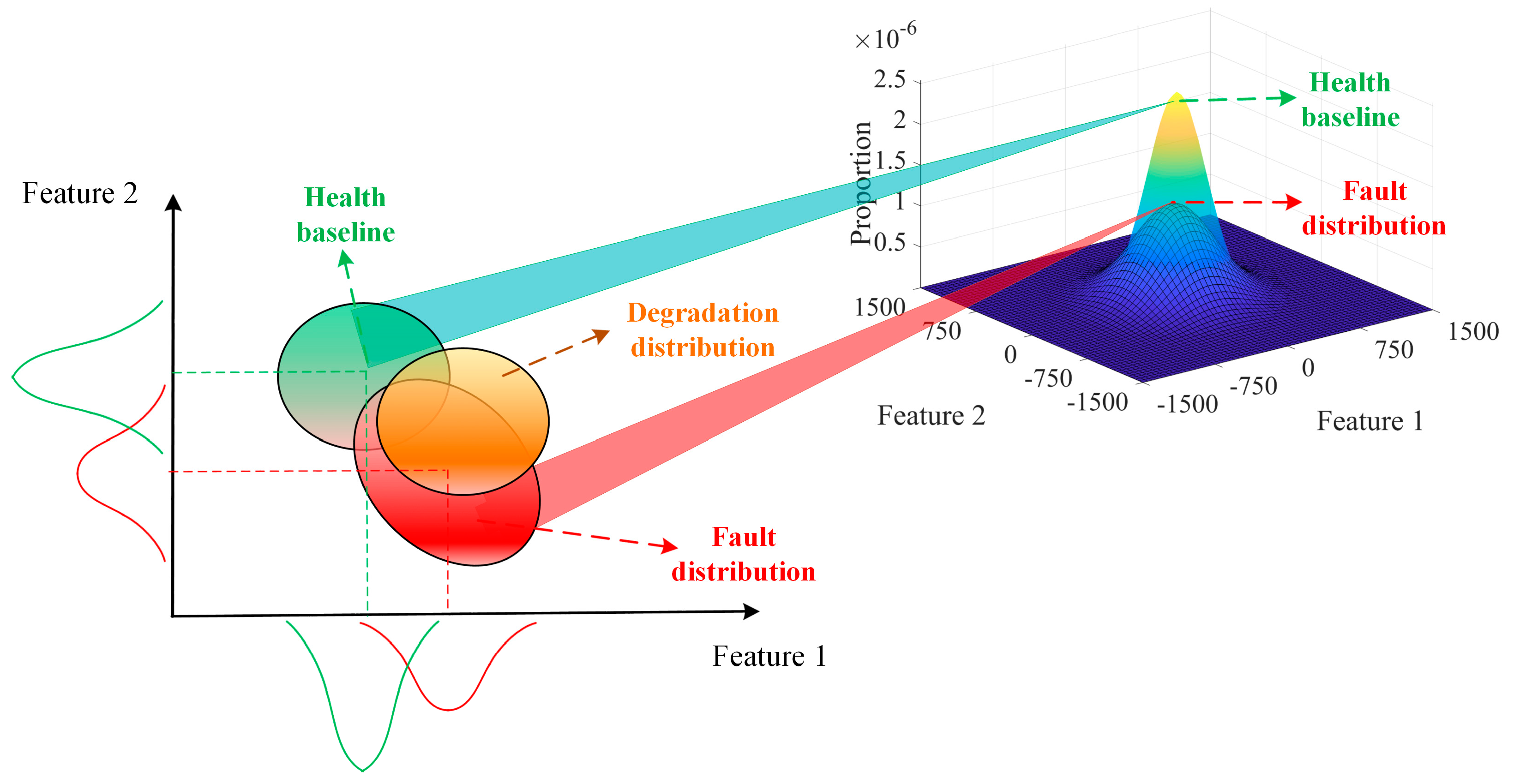
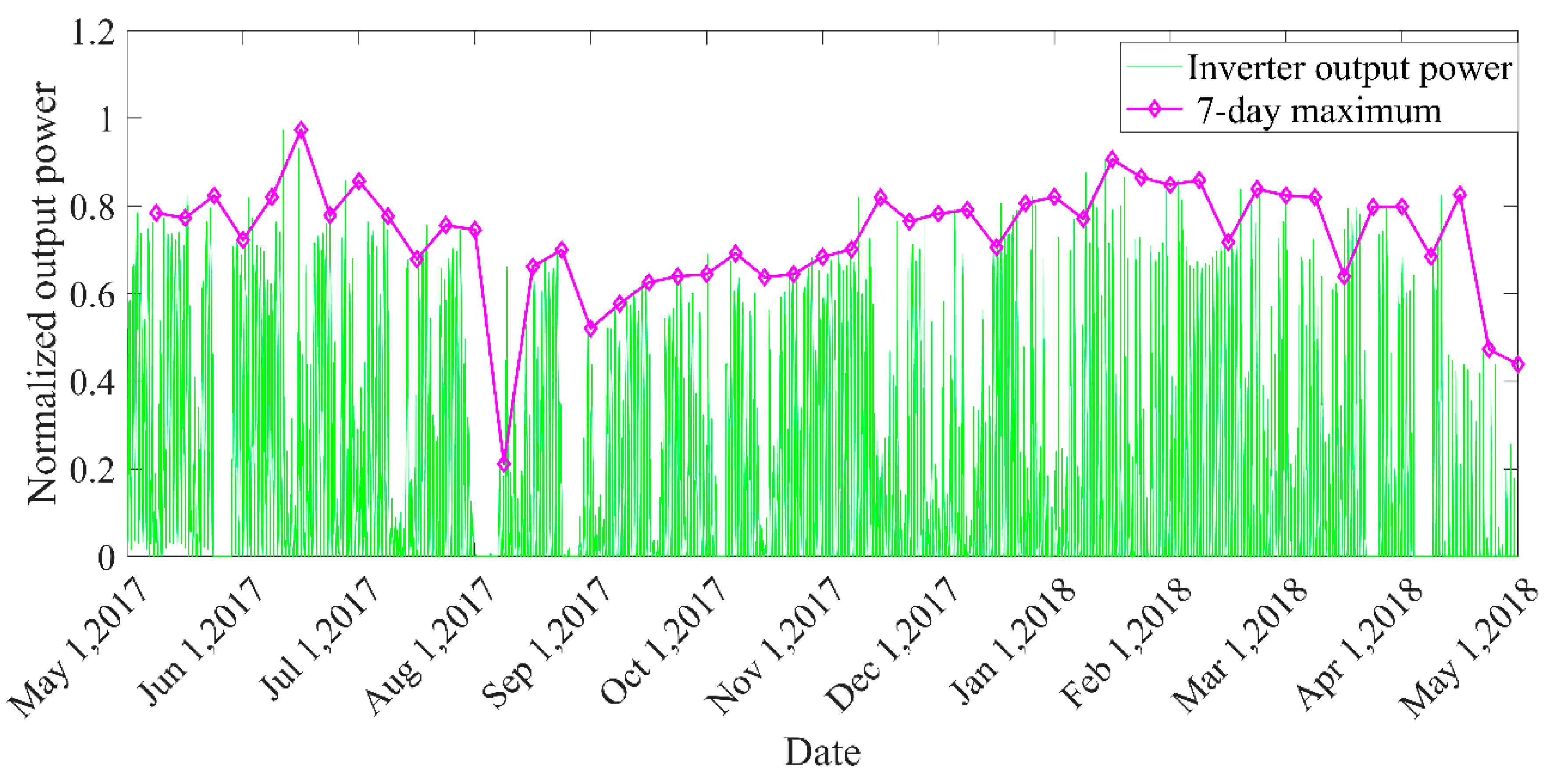
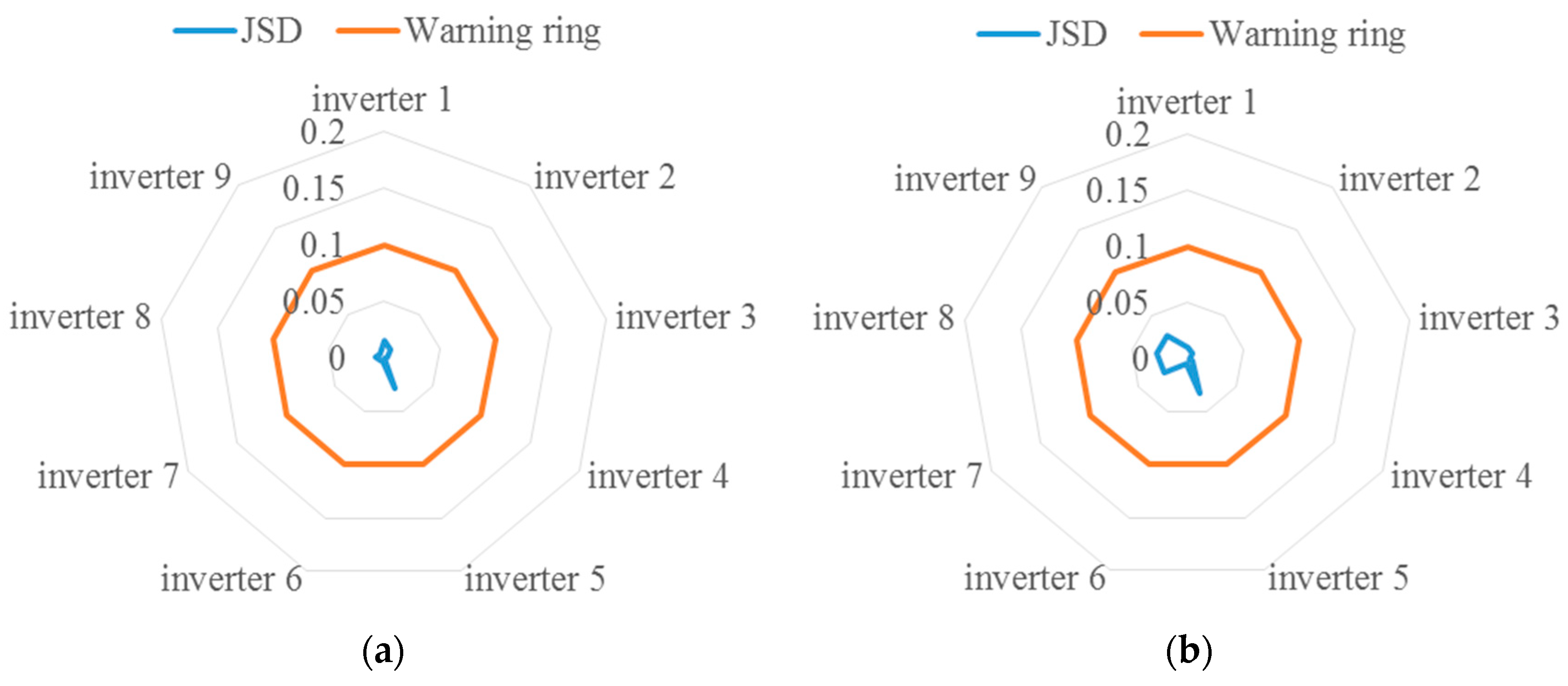
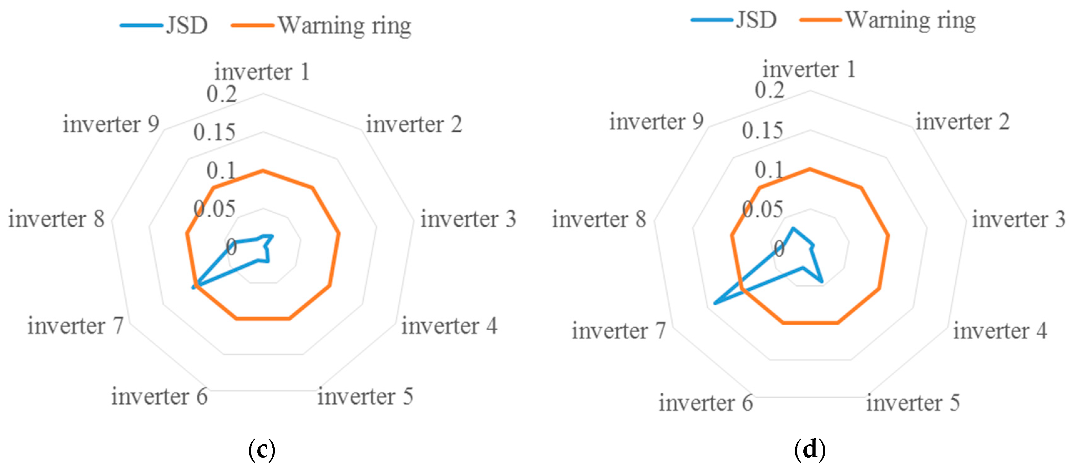
Robustness. Usually, the health baseline is directly established by the initial state of the equipment [10,11,12,34]. This paper sets up the health baseline based on the inverter group center. It can be seen from Figure 6 that the parameters of PV inverter are easily affected by season, sunshine, and other environmental factors. Observing Figure 7, we can see that for a single inverter, its characteristic distribution interval is also inevitably affected by the season factor. This will eventually lead the health indicator to be affected by the season factor. Observing Figure 10 and Figure 11, the performance degradation (JSD) of each inverter shows a good, gradually increasing trend since the health baseline is established based on the inverter group. It can be seen that the influence of environmental factors is effectively reduced. The reason is that the inverter to be predicted and the central inverter are in the same working condition all the time. In this respect, the method of establishing the health baseline in this paper has good robustness;
(2)
Quantification. This paper proposed a quantitative health indicator for the inverter. The difference between different feature distributions in the Gaussian mixture model is quantified through JSD, and then the health indicator is calculated. Figure 11 shows that the performance degradation (JSD) of each inverter shows a good, gradually increasing trend. Figure 13 shows that the proposed health indicator (overlap rate) can be effectively used to evaluate the inverter status;
(3)
Practicability. The on-site debugging of algorithm parameters is a huge challenge, which leads to poor applicability of algorithms with too many debugging parameters in the field [35]. For the fault prognostics method proposed in this paper, there is only one parameter that needs to be manually set: the early warning line. The value of the early warning line should be combined with the on-site operating conditions and refer to the health indicator range of the entire inverter group. Figure 13 shows that the proposed method accurately realizes the early warning of inverter failure. In brief, the proposed method is of great practicability in the field.
Meanwhile, there are still some challenges in the proposed method. As we know, it is a common phenomenon to discover multiple fault types in the PV system. Although the proposed method can predict the occurrence of a fault in advance, it is difficult to accurately determine the type of the fault. For this purpose, the fault diagnosis method based on the physical model [15,16,17] has advantages compared with the proposed method.

5. Conclusions

This paper presented a novel fault prognostics method for the PV inverter group. Each of the inverter’s features was extracted with the t-SNE method from the monitoring parameters. Then, the status of the inverter located in the feature distribution center was chosen as the health baseline of the whole PV inverter group. This approach made full use of the group deployment characteristics of PV inverters. Compared with directly selecting the initial performance of each inverter as the individual specific health baseline, selecting the center inverter to establish the health baseline avoided the problem of the inverter’s monitoring parameters being affected by various environmental factors, and this also eliminated the impact of the inverter’s initial performance differences. The experimental results show that the proposed method has various advantages in relation to robustness, quantification, and practicability. The fault prognostics algorithm successfully predicted the occurrence of an inverter fault 3 months in advance. Some conclusions are as follows:
(1)
The PV inverter’s main monitoring parameters, such as output power, are easily affected by environmental factors. This means that directly using the initial performance of the PV inverter as a health baseline is undesirable. Establishing the health baseline based on the inverter group center can effectively reduce the influence of environmental factors;
(2)
By way of searching the center of the PV inverter group, the health baseline can be established and treated as a data cluster of the Gaussian mixture model. Then, the feature probability distribution of the PV inverter to be evaluated forms another data cluster. The change trend of two data clusters’ divergence is consistent with the trend of equipment performance degradation;
(3)
To quantify the divergence of the Gaussian mixture model, we can calculate JSD of different data clusters in the Gaussian mixture model. After this, the overlap rate can be deduced from JSD and used for fault prognostics;
(4)
The setting of an early warning line is critical for fault prognostics. When there are different types of inverters in the inverter group, it is difficult to judge the abnormal state under all working conditions by setting the early warning line to a fixed value. In the future, we will combine the physical model of the PV system to conduct a more in-depth study on the dynamic setting method of the early warning line.

Author Contributions

Conceptualization, Z.H. and X.Z.; methodology, X.Z. and C.L.; validation, X.Z., C.L. and T.H.; formal analysis, Z.H.; investigation, T.H.; resources, Z.H.; data curation, X.Z.; writing—original draft preparation, Z.H. and T.H.; writing—review and editing, X.Z. and C.L.; visualization, X.Z.; supervision, T.H.; project administration, X.Z.; funding acquisition, C.L. All authors have read and agreed to the published version of the manuscript.

Funding

This research was funded by the National Natural Science Foundation of China, grant number 11802152.

Acknowledgments

The authors wish to thank the anonymous referees for their reviews and suggested improvements to the manuscript.

Conflicts of Interest

The authors declare no conflict of interest.

References

  1. Ghenai, C.; Bettayeb, M. Modelling and performance analysis of a stand-alone hybrid solar PV/Fuel Cell/Diesel Generator power system for university building. Energy 2019, 171, 180–189. [Google Scholar] [CrossRef]
  2. Mishra, M.K.; Lal, V.N. An improved methodology for reactive power management in grid integrated solar PV system with maximum power point condition. Sol. Energy 2020, 199, 230–245. [Google Scholar] [CrossRef]
  3. Ghenai, C.; Salameh, T.; Merabet, A. Technico-economic analysis of off grid solar PV/Fuel cell energy system for residential community in desert region. Int. J. Hydrog. Energy 2020, 45, 11460–11470. [Google Scholar] [CrossRef]
  4. Li, S. A variable-weather-parameter MPPT control strategy based on MPPT constraint conditions of PV system with inverter. Energy Convers. Manag. 2019, 197, 111873. [Google Scholar] [CrossRef]
  5. Vavilapalli, S.; Umashankar, S.; Sanjeevikumar, P.; Ramachandaramurthy, V.K.; Mihet-Popa, L.; Fedak, V. Three-stage control architecture for cascaded H-Bridge inverters in large-scale PV systems–Real time simulation validation. Appl. Energy 2018, 229, 1111–1127. [Google Scholar] [CrossRef]
  6. Dogga, R.; Pathak, M.K. Recent trends in solar PV inverter topologies. Sol. Energy 2019, 183, 57–73. [Google Scholar] [CrossRef]
  7. Ankit; Sahoo, S.K.; Sukchai, S.; Yanine, F.F. Review and comparative study of single-stage inverters for a PV system. Renew. Sustain. Energy Rev. 2018, 91, 962–986. [Google Scholar] [CrossRef]
  8. Tariq, M.S.; Butt, S.A.; Khan, H.A. Impact of module and inverter failures on the performance of central-, string-, and micro-inverter PV systems. Microelectron. Reliab. 2018, 88, 1042–1046. [Google Scholar] [CrossRef]
  9. Cupertino, A.F.; Lenz, J.M.; Brito, E.M.; Pereira, H.A.; Pinheiro, J.R.; Seleme Jr, S.I. Impact of the mission profile length on lifetime prediction of PV inverters. Microelectron. Reliab. 2019, 100, 113427. [Google Scholar] [CrossRef]
  10. Garoudja, E.; Harrou, F.; Sun, Y.; Kara, K.; Chouder, A.; Silvestre, S. Statistical fault detection in photovoltaic systems. Sol. Energy 2017, 150, 485–499. [Google Scholar] [CrossRef]
  11. Fazai, R.; Abodayeh, K.; Mansouri, M.; Trabelsi, M.; Nounou, H.; Nounou, M.; Georghiou, G.E. Machine learning-based statistical testing hypothesis for fault detection in photovoltaic systems. Sol. Energy 2019, 190, 405–413. [Google Scholar] [CrossRef]
  12. Yi, Z.; Etemadi, A.H. Line-to-line fault detection for photovoltaic arrays based on multiresolution signal decomposition and two-stage support vector machine. IEEE Trans. Ind. Electron. 2017, 64, 8546–8556. [Google Scholar] [CrossRef]
  13. Ameur, A.; Berrada, A.; Loudiyi, K.; Aggour, M. Forecast modeling and performance assessment of solar PV systems. J. Clean. Prod. 2020, 267, 122167. [Google Scholar] [CrossRef]
  14. Basnet, B.; Chun, H.; Bang, J. An Intelligent Fault Detection Model for Fault Detection in Photovoltaic Systems. J. Sens. 2020, 6960328. [Google Scholar] [CrossRef]
  15. Huang, C.; Wang, L. Simulation study on the degradation process of photovoltaic modules. Energy Convers. Manag. 2018, 165, 236–243. [Google Scholar] [CrossRef]
  16. Chin, V.J.; Salam, Z.; Ishaque, K. An accurate modelling of the two-diode model of PV module using a hybrid solution based on differential evolution. Energy Convers. Manag. 2016, 124, 42–50. [Google Scholar] [CrossRef]
  17. Zegaoui, A.; Aillerie, M.; Petit, P.; Charles, J.P. Universal Transistor-based hardware of photovoltaic generators SIMulator for real time simulation. Sol. Energy 2016, 134, 193–201. [Google Scholar] [CrossRef]
  18. Gu, J.; Wang, Y.; Xie, D.; Zhang, Y. Wind Farm NWP Data Preprocessing Method Based on t-SNE. Energies 2019, 12, 3622. [Google Scholar] [CrossRef] [Green Version]
  19. Zheng, J.; Jiang, Z.; Pan, H. Sigmoid-based refined composite multiscale fuzzy entropy and t-SNE based fault diagnosis approach for rolling bearing. Measurement 2018, 129, 332–342. [Google Scholar] [CrossRef]
  20. Maaten, L.V.D.; Hinton, G. Visualizing data using t-SNE. J. Mach. Learn. Res. 2008, 9, 2579–2605. [Google Scholar]
  21. Agis, D.; Pozo, F. A frequency-based approach for the detection and classification of structural changes using t-SNE. Sensors 2019, 19, 5097. [Google Scholar] [CrossRef] [PubMed] [Green Version]
  22. Wu, D.; Huang, Y.; Chen, H.; He, Y.; Chen, S. VPPAW penetration monitoring based on fusion of visual and acoustic signals using t-SNE and DBN model. Mater. Des. 2017, 123, 1–14. [Google Scholar] [CrossRef]
  23. Rodriguez, A.; Laio, A. Clustering by fast search and find of density peaks. Science 2014, 344, 1492–1496. [Google Scholar] [CrossRef] [Green Version]
  24. Wang, Y.; Wang, D.; Pang, W.; Miao, C.; Tan, A.H.; Zhou, Y. A Systematic Density-based Clustering Method Using Anchor Points. Neurocomputing 2020, 400, 352–370. [Google Scholar] [CrossRef]
  25. Gong, C.; Su, Z.G.; Wang, P.H.; Wang, Q. Cumulative belief peaks evidential K-nearest neighbor clustering. Knowl. Based Syst. 2020, 200, 105982. [Google Scholar] [CrossRef]
  26. Avendano-Valencia, L.D.; Fassois, S.D. Damage/fault diagnosis in an operating wind turbine under uncertainty via a vibration response Gaussian mixture random coefficient model based framework. Mech. Syst. Signal Process. 2017, 91, 326–353. [Google Scholar] [CrossRef]
  27. Sun, H.; Wang, S. Measuring the component overlapping in the Gaussian mixture model. Data Min. Knowl. Discov. 2011, 23, 479–502. [Google Scholar] [CrossRef]
  28. Zhang, J.; Yan, J.; Infield, D.; Liu, Y.; Lien, F.S. Short-term forecasting and uncertainty analysis of wind turbine power based on long short-term memory network and Gaussian mixture model. Appl. Energy 2019, 241, 229–244. [Google Scholar] [CrossRef] [Green Version]
  29. Gisbrecht, A.; Schulz, A.; Hammer, B. Parametric nonlinear dimensionality reduction using kernel t-SNE. Neurocomputing 2015, 147, 71–82. [Google Scholar] [CrossRef] [Green Version]
  30. Li, M.A.; Luo, X.Y.; Yang, J.F. Extracting the nonlinear features of motor imagery EEG using parametric t-SNE. Neurocomputing 2016, 218, 371–381. [Google Scholar] [CrossRef]
  31. Zhang, X.; Jiang, D.; Han, T.; Wang, N.; Yang, W.; Yang, Y. Rotating machinery fault diagnosis for imbalanced data based on fast clustering algorithm and support vector machine. J. Sens. 2017, 2017, 8092691. [Google Scholar] [CrossRef] [Green Version]
  32. Kim, T.; Lee, G.; Youn, B.D. PHM experimental design for effective state separation using Jensen–Shannon divergence. Reliab. Eng. Syst. Saf. 2019, 190, 106503. [Google Scholar] [CrossRef]
  33. Zhang, X.; Delpha, C.; Diallo, D. Incipient fault detection and estimation based on Jensen–Shannon divergence in a data-driven approach. Signal Process. 2020, 169, 107410. [Google Scholar] [CrossRef]
  34. Lee, J.; Wu, F.; Zhao, W.; Ghaffari, M.; Liao, L.; Siegel, D. Prognostics and health management design for rotary machinery systems—Reviews, methodology and applications. Mech. Syst. Signal Process. 2014, 42, 314–334. [Google Scholar] [CrossRef]
  35. Lei, Y.; Li, N.P.; Guo, L.; Li, N.B.; Yan, T.; Lin, J. Machinery health prognostics: A systematic review from data acquisition to RUL prediction. Mech. Syst. Signal Process. 2018, 104, 799–834. [Google Scholar] [CrossRef]
Figure 1. Main technical framework of this paper.
Energies 13 04901 g001
Figure 2. Main circuit of the photovoltaic (PV) power generation system.
Energies 13 04901 g002
Figure 3. Formulation and utilization of the monitoring data.
Energies 13 04901 g003
Figure 4. Schematic diagram of the feature distribution.
Energies 13 04901 g004
Figure 5. Flow chart of fault prognostics.
Energies 13 04901 g005
Figure 6. Normalized output power and weekly maximum of an inverter throughout a year.
Energies 13 04901 g006
Figure 7. Feature probability distribution of an inverter in different periods.
Energies 13 04901 g007
Figure 8. Process of searching the feature distribution center: (a) feature distribution of nine inverters; (b) decision graph; (c) the value of γ in decreasing order.
Energies 13 04901 g008
Figure 9. Proportion of times that different inverters were chosen as the center inverter.
Energies 13 04901 g009
Figure 10. Gaussian mixture model between the center inverter and the PV inverter to be evaluated: (a) inverter 4 in May 2017; (b) inverter 7 in May 2017; (c) inverter 4 in November 2017; (d) inverter 7 in November 2017; (e) inverter 4 in April 2018; (f) inverter 7 in April 2018.
Energies 13 04901 g010aEnergies 13 04901 g010b
Figure 11. Prognostics radar charts of inverters in different periods: (a) inverters in May 2017; (b) inverters in November 2017; (c) inverters in January 2018; (d) inverters in April 2018.
Energies 13 04901 g011aEnergies 13 04901 g011b
Figure 12. Feature distribution projections: (a) inverter 7 in January 2018; (b) inverter 7 in April 2018.
Energies 13 04901 g012aEnergies 13 04901 g012b
Figure 13. Fault prognostics for inverter 7 using the overlap rate.
Energies 13 04901 g013
Table 1. Common faults of the PV power generation system.
Fault TypeCause
anomaly of PV stringshielding of PV panel or degradation of PV string
anomaly of DC circuitDC current protection
anomaly of inverter circuitinverter current protection
grid connection faultcomponent damage, etc.
communication faultcommunication circuit damaged or disturbed

