Capacity and Impedance Estimation by Analysing and Modeling in Real Time Incremental Capacity Curves

Abstract

The estimation of lithium ion capacity fade and impedance rise on real application is always a challenging work due to the associated complexity. This work envisages the study of the battery charging profile indicators (CPI) to estimate battery health indicators (capacity and resistance, BHI), for high energy density lithium-ion batteries. Different incremental capacity (IC) parameters of the charging profile will be studied and compared to the battery capacity and resistance, in order to identify the data with the best correlation. In this sense, the constant voltage (CV) step duration, the magnitudes of the IC curve peaks, and the position of these peaks will be studied. Additionally, the behaviour of the IC curve will be modeled to determine if there is any correlation between the IC model parameters and the capacity and resistance. Results show that the developed IC parameter calculation and the correlation strategy are able to evaluate the SOH with less than 1% mean error for capacity and resistance estimation. The algorithm has been implemented on a real battery module and validated on a real platform, emulating heavy duty application conditions. In this preliminary validation, 1% and 3% error has been quantified for capacity and resistance estimation.

1. Introduction

The performance of a lithium ion battery is reduced over its lifetime due to irreversible physical and chemical changes in the internal structure. In the case of lithium ion batteries, the degradation is caused by several mechanisms [1] such as loss of active materials, the growth of solid electrolyte interface (SEI) layers, electrode structural disordering and electrolyte decomposition. In this sense, identification of the battery aging mechanism might be challenging [2], since those mechanisms are strongly coupled during the aging process. Therefore, those mechanisms cannot be isolated and studied independently. Considering the state of the art, the main aging mechanisms can be classified into three groups: loss of lithium inventory (LLI), reduction of the active material on the positive electrode (PE), and the reduction of the active material on the negative electrode (NE). In the first case, the available lithium ions are reduced due to surface film formation (SEI growth), lithium plating, and decomposition reactions. Consequently, fewer ions are accessible for a chemical reaction, reducing the capacity of the battery. In the PE, due to structural disordering and particle cracking, the active material of the PE available for the chemical reaction is reduced over its lifetime. Finally, a similar process occurs on the NE: the active material of the NE is reduced. The electrolyte is also prone to decomposition; a part of the electrolyte is also consumed in the formation of electrode–electrolyte interphases during cycling, leading to a performance reduction. As a consequence of these mechanisms, the performance is reduced over the lifetime of the battery.

As a consequence of those aging mechanisms, the capacity and the internal resistance are damaged [3], leading to the reduction of the battery’s energy and power density. In this sense, the battery performance reduction will advance to a critical level, where the battery will not be able to meet the application requirements. From a proper battery monitoring point of view, capacity fade is directly correlated with the state of charge (SoC), state of health (SoH) and lifetime estimations, since the value of this parameter is used for both calculations [4]. Moreover, to estimate the maximum charging or discharging current rate that the battery is able to charge and discharge, quantified by the state of function (SOF), accurate impedance estimation is mandatory. Therefore, incorrect impedance estimation will affect negatively the SOF estimation accuracy. Consequently, in order to predict the end of life and to estimate the different inner states of batteries accurately, it is very important to understand the aging of a battery and to identify the values of these variables continuously.

In this sense, the health of a battery usually is quantified by taking the relation between the current and initial capacity. Since the capacity is reduced due to the aging effect, the health indicator is reduced as well over the lifetime. Additionally, the impedance rise is another important indicator for evaluating the health of a battery, especially for those applications where the battery is exposed to high current rates. Depending on the final application specifications, the end of life can be limited by a capacity fade or impedance rise; hence, it is important to track both. In the literature, the SOH estimation has been proposed using two different main approaches or strategies such as data-driven and adaptive systems. Extensive testing, comprehension, and correlation between the testing conditions and aging indicators is necessary to estimate the aging following a data-driven strategy (based on measuring the necessary indicators such as Ah or Wh and executing the models), with the corresponding cost of testing and required time. Additionally, if the battery is being used in a different condition from the lab testing, the estimation can diverge from the real state. Within the adaptive strategies, in some publications, the SOH has been quantified by measuring the internal resistance [5,6,7], but it is difficult to have an accurate measurement due to the synchronization and accuracy needed for measuring current and voltage. As an alternative, some adaptive systems that evaluate the degradation of the battery have been proposed. Some of these variables are measurable such as voltage and current, but some others need to be estimated since these are not measurable. The SOC and SOH are normally estimated using adaptive or statistical inference techniques. In this sense, there are several ways to estimate the SOH, e.g., Kalman filter (KF), extended Kalman filter (EKF) [8], genetic algorithm (GA) [9], particle filter [10], fuzzy logic [11], artificial neural networks (ANNs) [12], and the least-squares method (LSM) [13].

The EKF strategy has been widely used for different purposes such as SOC, SOH, and also for prognosis. He et al. [14] used a dynamic Electro Motive Force (EMF) curve updated by using recursive least squares (RLS); then, this information was used within the EKF to estimate the SOC based on the updated open circuit voltage (OCV) curve. Chen et al. [9] used genetic algorithm (GA) to update the Li-ion equivalent electric circuit parameters: ohmic resistance and diffusion resistance and capacitance. In this work, Chen used the evolution of the diffusion capacitance to update the SOH of a battery. Nevertheless, the high volume of the operations and the consequent high computational cost make the implementation of these algorithms challenging for real-time implementation [15]. Additionally, an incorrect estimation of one of the aforementioned variables affects negatively the estimation of other variables, since they are correlated to each other. In this sense, additional work has been [16] observed for estimating the internal impedance dynamically and implementing projection techniques [4] to estimate the SOH of the batteries. In this work particularly, the dynamic impedance is defined as the changes in voltage generated by the current change during the charging/discharging process. However, the SOH accuracy was not described in that paper. Based on electrochemical principles, since both the cathode and anode are reduced or blocked, leading to capacity fade, some other authors suggest evaluating battery aging based on the OCV–SOC curve, which is observed at a low current rate [17]. However, this strategy requires charging and discharging a battery at controlled conditions and at very low rates (e.g., 1/25 C). This alternative cannot be used in a real application due to the long time needed. The results of these techniques are very accurate but unfortunately, these methods cannot meet the online real-time requirements for BMSs. Alternatively, some SOH estimation strategies have been proposed in [14,18,19] using real-time equivalent model adaptive systems, based on optimization strategies, with the corresponding high computational cost.

Incremental capacity analysis (ICA) is an interesting tool to estimate the capacity of a battery, since it only requires tracking the charging profile in static conditions. From the application point of view, the charging current or power can be managed and controlled by the battery management system (BMS), regardless which charger is used, since the process is defined by the BMS. The intercalation of the lithium metal analysis leads to the correlation of the ICA and capacity, demonstrating the sensitivity of this charging profile to the aging of the battery [20,21]. In this sense and according to several authors [22,23], this tool can be used to analyze the evolution of the capacity. Wang et al. used their ICA with the support vector machine (SVM) model to reduce the number of operations and to predict the SOH of a cell. According to the results, the algorithm was able to estimate the capacity within a 1% error bound [24]. To reduce further the computational cost of this tool, smooth tools [22] such as Gaussian processes with relatively low computational cost were proposed to compute the incremental capacity (IC) curve from the measurements. Furthermore, in these papers, only the capacity fade was taken into consideration for SOH determination, not considering the impedance rise experimented by the cells. Furthermore, a Gaussian process was used to smooth the calculated IC curve, which is still very heavy to compute.

To overcome the aforementioned issues, the objective of this work is to evaluate different online and computationally low-cost techniques for capacity and impedance estimation, based on the study of the battery charging profile. In order to evaluate these techniques in batteries aged at various conditions, extensive aging test matrix and aging check test procedures are proposed. A methodology to calculate the optimum IC curve is proposed, using a very simple algorithm. Then, correlation between different charging profile indicators (CPI) and battery health indicators (BHI) will be studied, in order to identify the best CPI to estimate both BHI: capacity and resistance. In this sense, the added value of this work comes from the low cost of the algorithm IC calculation, since a very simple strategy has been used to smooth the IC curve. Additionally, this paper proposes the estimation of both main aging indicators such as capacity and resistance.

2. Cell Level Tests

To test the cell samples, a Basytec tester (HPS.X.62.44.0502) associated to a climatic chamber (VÖTSCH VC34100) to control the temperature is used. Using these two devices, it is possible to control and measure variables such as cell temperature, current, and voltage.

2.1. Cell Specifications

The most important feature of the selected cell for this work is the high energy density of 240 Whkg⁻¹. It presents a nominal capacity of 54 Ah, and the working voltage range is limited to 2.5–4.15 V, as recommended by the manufacturer. According to the data sheet, the negative electrode is made of graphite, and the positive electrode is composed of Li(NiMnCo)O₂. The maximum current rate is limited to 1 C, and a nominal charging rate is recommended to conduct at a C/2 rate. The most important features are summarized in

Table 1. Cell specifications.

Capacity	Material	Maximum Continuous Current		Voltage Range	Temperature Range
54 Ah	Li(NiMnCo)O2)carbon	C/2 Charge	1 C Discharge	2.5–4.15 V	10–45 °C

.

2.2. Aging Test Matrix Definition

In order to evaluate the BHI estimation techniques, the capacity fade, and the impedance rise, an extensive test matrix was designed. The goal of this test matrix was to analyze the lifetime of this particular battery technology and to identify a proper strategy to estimate BHI when the cell is aged at various cycling conditions. In this sense, two samples were used in each test conditions in order to get stronger results. All conducted cycling tests are detailed in

Table 2. Cell aging test matrix.

N°	Temperature	Charge Voltage	DoD	Discharging Rate	Charging Rate
1	25 °C	4.15 V	90%	1 C	C/3
2	10 °C	4.15 V	90%	1 C	C/3
3	45 °C	4.15 V	90%	1 C	C/3
4	25 °C	4.15 V	90%	1 C	C/2
5	25 °C	4.15 V	90%	C/2	C/2
6	25 °C	4.15 V	90%	Automotive power profile
7	10 °C	4.15 V	90%	Automotive power profile
8	45 °C	4.15 V	90%	Automotive power profile

. According to this table, three temperature levels were selected to analyze the effect of this variable: 10, 25, and 45 °C. The depth of discharge (DoD) is kept constant at 90%, which is a requirement of the application. The DoD is calculated considering the discharged Ah referring to the current capacity value. Hence, 90% DoD is calculated by multiplying 0.9 by the last measured capacity value. To avoid errors caused by the current error accumulation on the Ah counting, in every charge after a conventional CC–CV (constant current–constant voltage) charge, the SOC was reset to 100%. Generally, constant current cycles were performed. The discharge current rate was set to 1 C in the entire test, except for one case, where it was reduced to C/2. Similarly, the charging rate of the constant current phase was predefined to C/3, with two additional tests at C/2. The aim of this modification is to investigate the effect of charging and discharging current rates on aging.

Additionally, a typical heavy-duty power profile scaled down to the cell level was applied at different temperatures in order to compare the aging across a range of the expected operating temperatures. This power profile consisted of 16 h of heavy-duty vehicle usage, containing discharging and charging current peaks, with an equivalent discharge of 85% DoD at the beginning of life. Then, the cell was charged at a C/3 rate to 4.15 V and kept at this voltage until the current was below 0.05 C. Finally, the cell rested for approximately 3 h to complete 24 h cycle with the discharge, charge, and rest period. The evolution of each battery capacity and impedance over the lifetime is visualized in Figure 1.

2.3. Aging Check Test Procedure and Battery Health Indicator Extraction

The aging check test (ACT) is visualized in Figure 2, it was designed to quantify BHI, and it was conducted at beginning of life, end of life, and in an interval of 4 weeks. Cell aging testing was finished when the cell capacity had decreased below 80% with respect to the initial value. In this work, the capacity and impedance are considered as the main health indicators, and therefore, the ACT was designed to obtain these values. In this sense, from each ACT, some parameters were extracted automatically such as the capacity, impedance at 1 C, and the OCV vs. SOC. To control the effect of the temperature on these measurements, the ACT tests were conducted within a climatic chamber at a constant temperature of 25 °C. To measure the capacity, firstly, a conventional charging step (0.5 C rate constant current until 4.15 V, constant voltage charge at 4.15 V until the current has decreased below 0.05 C rate) were applied. Then, a 0.5 C discharge until the minimum voltage of 2.5 V was performed in order to measure the current capacity, which was used to follow the evolution of the capacity over the lifetime. The resistances were calculated by applying a constant current pulse at different SOCs (95%, 90–10% in 10% steps and at 5%). At each SOC, a 60 s 1 C rate discharge pulse preceded and followed a 600 s rest period. The SOC change generated by this pulse during 60 s is 1.6%, which is not assumed to be big enough to consider impedance variation during this interval. For impedance rise identification, the 60 s discharge resistance R at 50% SOC was used for the aging analysis and tracking. This resistance value was calculated following Ohm’s law, with the measured voltage and current profiles during this pulse.

3. Charging Profile Indicator Extraction

To evaluate the correlation between each charging profile indicator (CPI) and BHI, a systematic battery test extraction has been implemented from each ACT, which is exported in an Excel file with all the measurements (voltage, current, temperature) together with additional information about the test. Then, all these results are analyzed with a script developed in Matlab in order to analyze which CPI presents the best correlation to the BHI. A general overview of the workflow is visualized in Figure 3. Firstly, the work will start by analyzing the correlation between constant voltage (CV in Section 3.1) step time and capacity/impedance. Then, the work will focus on identifying the optimum IC curve calculation strategy from voltage and current measurements (Section 3.2). From this IC curve, the correlation between the absolute peak, local peak, value at voltage threshold (4 V), and model parameter with the aforementioned health indicators will be investigated in Section 3.2.1, Section 3.2.2, Section 3.2.3 and Section 3.2.4, respectively.

3.1. Constant Voltage Step Time

The conventional charging procedure consists of two main steps. During the first step, a constant current (C/3) is applied to each cell until they reach the maximum charging voltage (4.15 V). Then, in a second step, each cell is kept at constant voltage until the cell current is decreased below 0.05 C. The constant voltage step time is considered in this work from the first cell voltage measurement higher than 4.145 V to the end of charging process, which is measured in seconds. Figure 4 represents the evolution of the voltage (subplot a) and the evolution of the IC curve over the lifetime, with the corresponding identification of IC local and maximum peaks. The results correspond to the cell aged at 25 °C, 1 C rate discharge, 0.3 C rate charge, and 90% DoD.

3.2. IC Calculation

The IC curve shape and the CPI obtained from this curve are strongly influenced by the measurement sample time and the derivation calculation strategy. In this particular work, the cell voltage, current, and temperature are measured every 30 s during the ACT charging process. Similarly, incremental capacity is calculated by differentiating the change in the charged capacity with respect to the change in terminal voltage during the charging process, as defined in Equation (1). Some other authors have used more sophisticated strategies such as Gaussian process [22] to smooth the shape of the IC curve. However, in order to reduce the computational cost of the calculation, the value of the IC curve is calculated by comparing two points displaced N measurements (Displacement). In this sense, two measurements displaced 30 points; the displacement in time between them is 30 × 30 in seconds. The objective is to identify the best displacement between two points used to calculate the IC curve, taking into account the correlation of CPI and BHI. This process is discussed in detail in Section 4.

$$IC=\frac{d{Q}_k}{d{V}_k}=\frac{Q_k-Q_{k-N}}{V_k-V_{k-N}}$$

(1)

Q: Charged ampere hour; V: Measured voltage; N: Displacement.

3.2.1. Absolute Maximum Value of IC Curve and the Position of the Peak

From each IC curve, the absolute maximum value is simply obtained by identifying its maximum peak. Additionally, the voltage of the cell at this point is recorded to take it as a supplementary potential aging indicator. The maximum absolute value is visualized with a blue star in Figure 4.

3.2.2. Local Maximum Value and the Position

From each IC curve, the local maximum value is obtained. To identify the local maximum value, the reduction of the IC curve slope is considered. To find this point automatically, the second derivation of the IC curve is calculated, as shown in Equation (2). In this curve, the local peak is identified when the IC curve derivation is changed from a value higher than 2 Ah/V² to a value that is lower. From this step, the value of the local peak and the voltage at this point of the IC curve are recorded for later study if there is any correlation with the BHI. This point is highlighted with a red star in Figure 4.

$$\frac{d^2 Q_k}{d{V}_k^2}>2\frac{Ah}{V^2}>\frac{d^2 Q_{k+1}}{d{V}_{k+1}^2}$$

(2)

3.2.3. IC Value at Voltage Threshold

The IC value at 4 V has been stored and considered as a candidate to use this CPI for estimating the aforementioned BHI, capacity, and resistance. This 4 V IC value has been selected after a visual inspection of the IC curve and identification as a potential candidate for BHI estimation. The IC value at 4 V is visualized with a green triangle in Figure 4.

3.2.4. IC Modeling

The equation used to describe the pseudo binary reactions that appear on the IC curve is detailed in Equation (3) [25], and the description of each parameter is detailed in

Table 3. Parameters used in the IC modeling.

Parameters	Description
$n$	Number of peaks used to model the IC curve (I = 1, …, n).
$A_i$	Pre-exponential factor (magnitude of the ith peak).
${\omega }_i$	Scale factor (the width at half height of ith peak).
$V_{0i}$	The symmetry center of the ith peak.
$V$	The input vector of the equation (the voltage range used).

. The measured IC curve is described by the convolution of the pseudo binary reactions in the positive electrode with the pseudo binary reactions in the negative electrode [26] over the voltage range. To find the IC model optimum parameters (A_i, V_oi, and ω_i) of each curve, the least square technique has been used, minimizing the difference between the measured and modeled IC curve. After analyzing the measured IC curve, a 6th-order model has been selected due to the suitability to fit with the measured curve.

$$\frac{dQ}{dV}={\displaystyle \sum }_{i=1}^n{A}_i{e}^{-\left(\frac{V-V_{0i}}{{\omega }_i}\right)}$$

(3)

The potential of modeling this IC curve is reported on the literature [27,28,29]. According to the authors, (1) it is possible to identify the aging mechanisms produced inside the cell; using this tool, it is possible to track the evolution of each process to determine the main aging mechanism, providing an opportunity to avoid those situations inducing this process. (2) The capacity of the battery can be calculated by integrating the modeled IC from the minimum voltage to the maximum one, and (3) it is possible to quantify the IC curve shape change numerically without any human intervention. The IC modeling has already been used in the literature, but the novelty of this work focuses on the correlation of the evolution of the parameters described in Table 3 with the BHI.

4. Results and Discussion

After describing all the BHI and the CPI extraction, the next step is to evaluate systematically the correlation between each aforementioned parameter (described in Section 3.1 and Section 3.2). All the cells used in the aging test matrix (defined in Section 2.2) are used to validate each SOH estimation strategy. Since the aging matrix has been designed to test under a wide current, temperature, and DoD spectrum, the algorithm will be tested out of ideal conditions. Beforehand, the best IC curve calculating strategy will be identified, avoiding high computational cost strategies and finding the optimum displacement points for executing Equation (3).

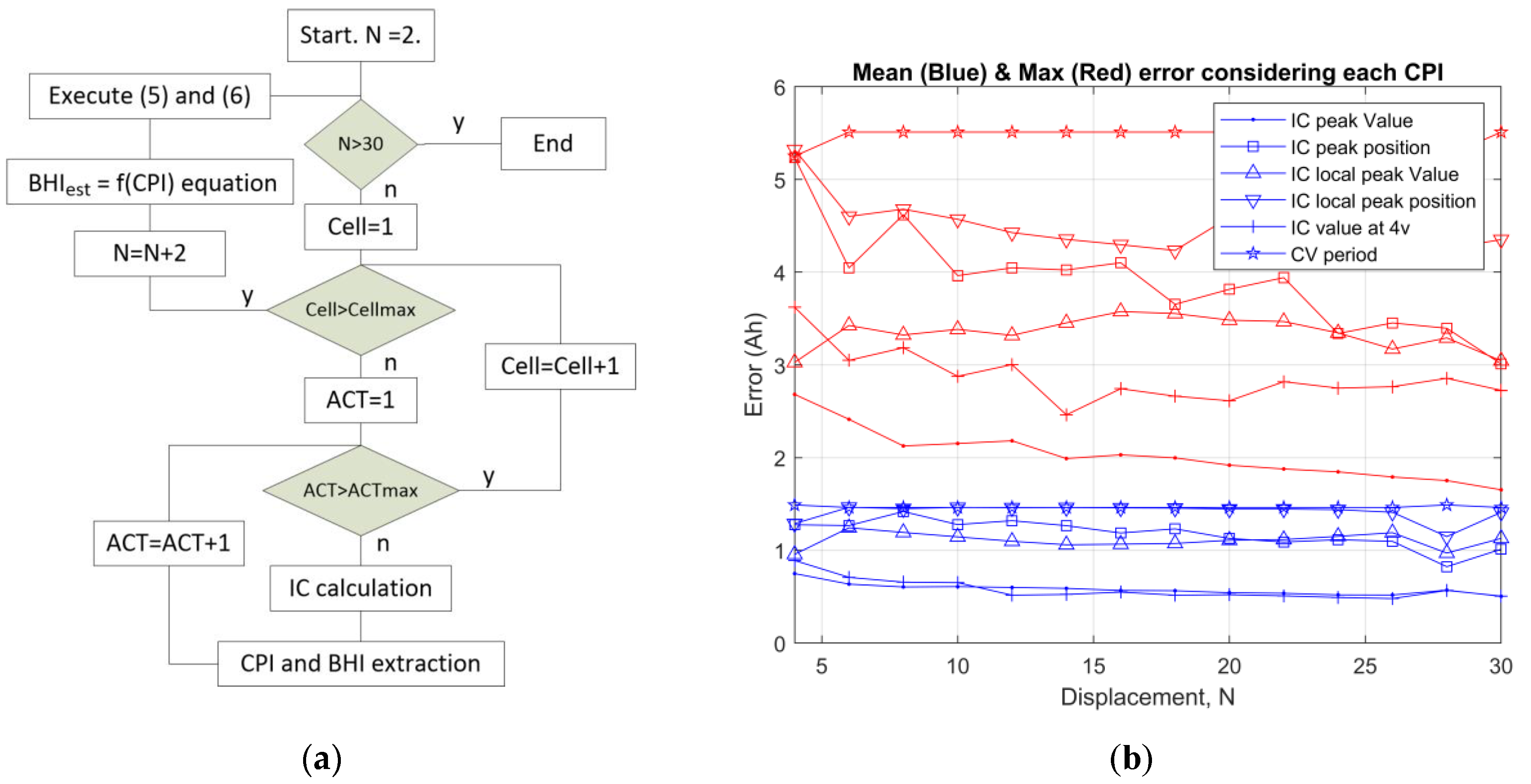
To reach this objective, the flowchart visualized in Figure 5a has been designed and executed. The algorithm starts with defining the initial displacement, limiting to 30 in order to avoid the usage of large arrays during the on-line implementation within a micro controller. The next two steps are focused on analyzing all the aging check tests of all the cells described in Table 3. In each ACT, the IC will be calculated, and from this curve, the CPI detailed in Section 3.2.1, Section 3.2.2, Section 3.2.3 and Section 3.2.4 are obtained. Additionally, the BHI (capacity and impedance at 50% of SOC) are calculated. When this CPI and BHI extraction is conducted for all the ACT and cells, the number of displacement N is increased, and the algorithm starts finding an equation to correlate each CPI and BHI. This is obtained by a second-order equation, which is described in Equation (4). The parameters (C₀, C₁, and C₂) used in the equations are found using least square technique to minimize the difference between the measured and calculated value. This equation is found for each CPI type detailed in Section 3.

$$BH{I}_{est}{}_i=C_{es{t}_i}=f\left(CPI\right)=C_{0, j}+C_{1,j }CP{I}_{j,i} +C_{2,j}CPI{ }_{j,i}^2$$

(4)

Afterwards, the accuracy of BHI estimation is evaluated by comparing to the BHI measured. From this comparison and using Equations (5) and (6), the mean and maximum error of the BHI estimation using each CPI is evaluated. In this sense, the mean (blue) and the maximum (red) values of the absolute error are shown in Figure 5b. Both of the errors are plotted for each displacement of the measurements, as stated in Equation (1), to calculate the IC curve (see Section 3.2). The objective is to identify the optimum IC curve calculation strategy for later use in capacity and resistance estimation.

$$Mea{n}_{error}=\frac{1}{N}{\displaystyle \sum }_{i=1}^n\left|{\mathrm{BHIest}}_i-{\mathrm{BHI}}_i\right|$$

(5)

$$Ma{x}_{error}=\max \left(\left(\left|{\mathrm{BHIest}}_i-{\mathrm{BHI}}_i\right|\right)\right), i=1,\dots ,n$$

(6)

According to the results shown in Figure 5b, the best indicator to estimate the capacity is to evaluate the peak value of the IC curve. Additionally, the best results are obtained if the IC curve is calculated taking two points displaced 30 sample points. Considering the sample time of 30 s during the charging step, the two voltages and Coulomb counting values to calculate the IC are distanced 900 s from each other. Going more in detail, there is not a big difference on the mean value error if we consider the accuracy obtained with the maximum and the IC value at 4 V. However, the maximum error considering the maximum value of the IC curve is reduced down to 1.7 (red IC peak value) Ah for all the cells and ACT studied in this work. Considering this CPI and N = 30, a mean value of 0.56 Ah (blue IC peak value) and maximum of 1.7 Ah are obtained, which means 1% and 3% respectively referring to the nominal capacity of the cell.

The outcomes of this section are as follows: (1) a methodology is proposed to identify a low-cost IC calculation strategy, avoiding the use of more complex Gaussian processes or similar filtering techniques; (2) the CPI with the highest correlation with the BHI is the maximum IC value, measured during the charging; (3) additionally, the estimation of both capacity and impedance is defined as a target of this work.

4.1. Capacity Fade Estimation Results

4.1.1. CV Step Duration

The correlation between capacity BHI and the CV step time duration is not very strong. The dispersion between the evaluated points is significantly higher among all the studied cells in this work, and consequently, the mean value of the error done in the capacity estimation increases up to 1.48 Ah. The maximum error has increased up to 5.5 Ah. Additionally, this technique could only be used in those applications using single cells, since in applications using more than one cell, the CV step could not be limited by a single cell. Therefore, the usage of this method is discarded for real-time implementations. Sun et al. [30] reached the same conclusion in their research.

4.1.2. IC Absolute and Local Peak Value

Figure 6 shows the correlation between the capacity and the CPI obtained from each ACT of each cell, which were aged according to the operation conditions defined in Table 2. Figure 6 shows the capacity vs. the measured maximum IC peak value in blue, the capacity vs. the local maximum value in red, and the value found when the cell presents a voltage of 4 V during the charging process in green. In a continuous line and at a corresponding color, the fitted equation is plotted using a second-order equation described in Equation (4). According to the results, a mean error value of 0.56 Ah was found using the maximum value, 0.81 Ah in case of the local maximum value, and 0.55 Ah using the value found at 4 V. For a new battery, the standard deviation could be larger than the indicated mean value. However, this deviation is reduced considerably when the capacity value is reduced, where estimation accuracy is more critical. The lowest error when estimating the BHI has been obtained using the maximum IC value, and therefore, the values found for the parameters C₀, C₁, and C₂ in this case are visualized in

Table 4. Capacity and impedance estimation equation parameter values.

Estimation Target	Values
Capacity vs. IC max value	$C_0=$21.62	$C_1=0.2849$	$C_2=-3.98\times {10}^{-4}$
Resistance vs. IC local max value	$R_0=8.3\times {10}^{-3}$	$R_1=-1.58\times {10}^{-4}$	$R_2=9.28\times {10}^{-7}$
Capacity vs. IC model max values	$C_0=29.9$	$C_1=0.241$	$C_2=-4\times {10}^{-4}$
Resistance vs. IC model local max values	$R_0=2.8\times {10}^{-4}$	$R_1$ = −1.63 × 10−5	$R_2=$3.27$\times {10}^{-8}$

. Some additional information is included in this table such as the parameters to calculate resistance considering the maximum IC value and the capacity/resistance using IC model parameters. The IC modeling results will be discussed in detail in Section 4.1.4 and Section 4.2.4.

As stated in the introduction, there might be several mechanisms reducing the battery performance, making the identification of what is reducing the IC peak value difficult. According to the literature [22], the most probable cause might be lithium plating, but specific equipment and post-mortem analysis is needed to identify the mechanism causing this change.

4.1.3. IC Absolute and Local Peak Position

Similarly, the correlation found between the IC peak (blue) and local peak (red) position is plotted in a second subplot of Figure 6. In this chart, the capacity is visualized with respect to the voltages or the position of the absolute and local peaks. To find an equation that meets the real capacity considering the different peak positions, a similar optimization strategy is used. In this case, the mean and the maximum error values were found to increase up to 0.76 Ah and 1.18 Ah, respectively. Compared to the accuracy obtained from the IC peak and local peak error, the estimation made using the local peak was found to be less accurate.

4.1.4. IC Modeling

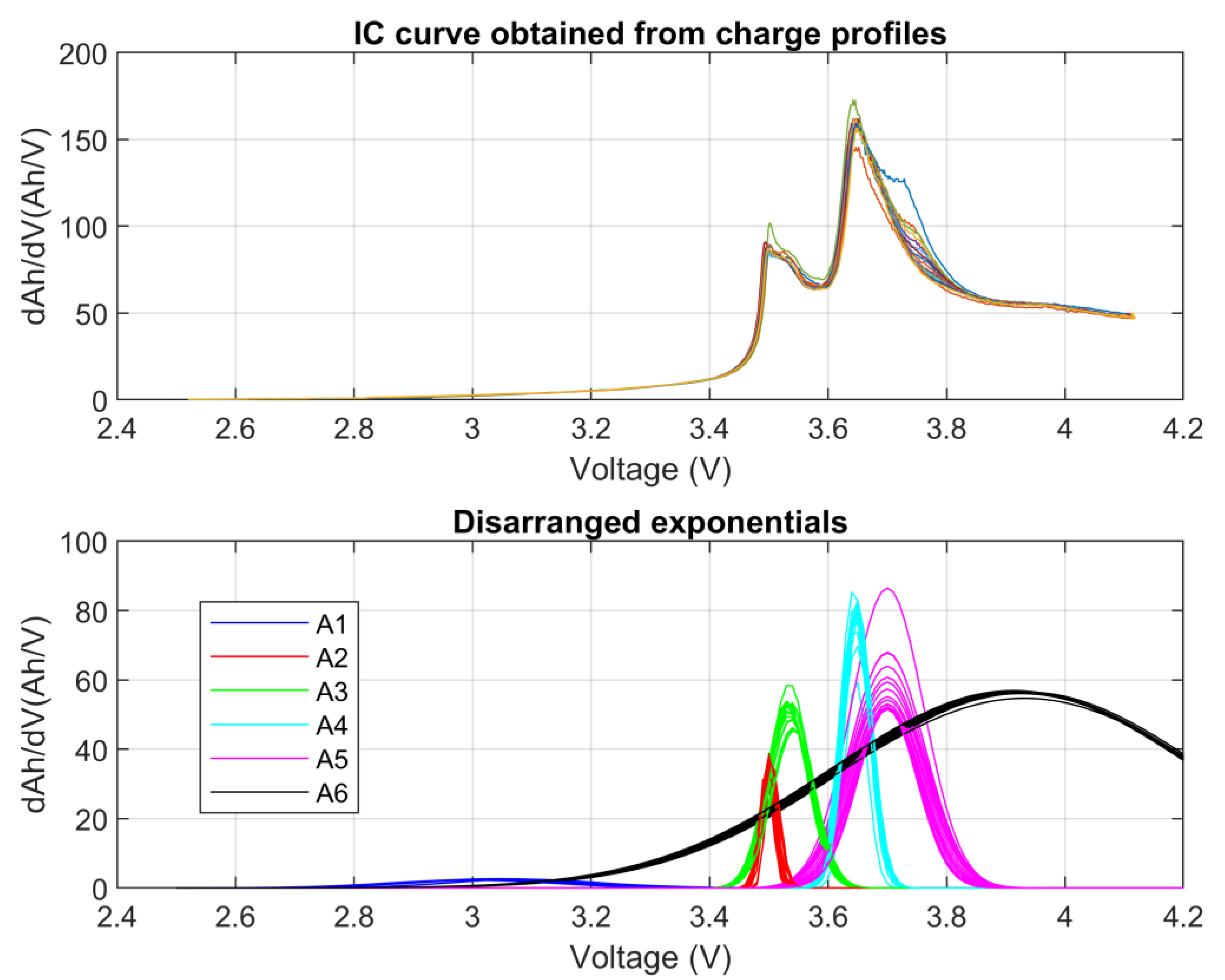
Following the steps defined in Section 3.2.4, each IC curve has been modeled by finding the optimum parameter model values for each disarranged exponential proposed in Equation (3). Taking into account the shape of the IC curve to model, a 6th-order IC model has been selected to fit with the real IC curve. Hence, a set of 18 parameters are found in each optimization (6 A, 6 V, and 6 ω) in order to minimize the real and modeled IC curves. As it has been previously mentioned in this work, the least square technique is used to find the optimum value of each parameter. The different IC curves and the evolution of each exponential curve are visualized in Figure 7. According to the experience acquired in this work, the maximum value of the IC curve was found to decrease proportionally to the capacity fade. In this sense, in the second subplot of Figure 7, the maximum value of the IC curve is modeled by the parameters A4 and A5, by observing the position of these two disarranged exponentials. The goal of this study is to identify if the representation of the IC peak using the model has the same correlation as the real IC peak value to the capacity.

Therefore, in Figure 8, the capacity was plotted vs. the sum of A4 and A5, since they represent the maximum value of the IC curve. According to the result, the correlation between both of the indicators is very strong, and this information can be used again to estimate the capacity of the battery in real application. Additionally, Figure 8 shows in a continuous red line the equation that describes this correlation, using a second-order polynomial definition in Equation (4). In this particular estimation, the mean value of the error during the capacity estimation was found to be 0.47 Ah, which is less than 1% with respect to the nominal capacity of this particular cell.

The estimation of the capacity using IC modeling presents a higher computational cost than evaluating simply the maximum value of the IC curve. However, tracking and modeling the IC curve offers great potential to evaluate another degradation mechanism [26]. In this specific work, during the best BHI identification technique, the algorithm was executed in a computer. More specifically, the IC peak magnitude and location might be used to evaluate the degradation, since the IC peaks represent the phase transitions during the intercalation/deintercalation processes, and this electrochemical reaction is affecting directly the capacity loss. The locations of the peaks might also have a correlation with the faded capacity and can give a good estimation of the loss. Particularly, with this battery diagnostic tool, it could be possible to identify the lithium plating phenomenon and anticipate the quick capacity fade produced by this. This investigation is considered out of this paper’s scope.

4.2. Resistance Growth Estimation

4.2.1. CV Step Duration

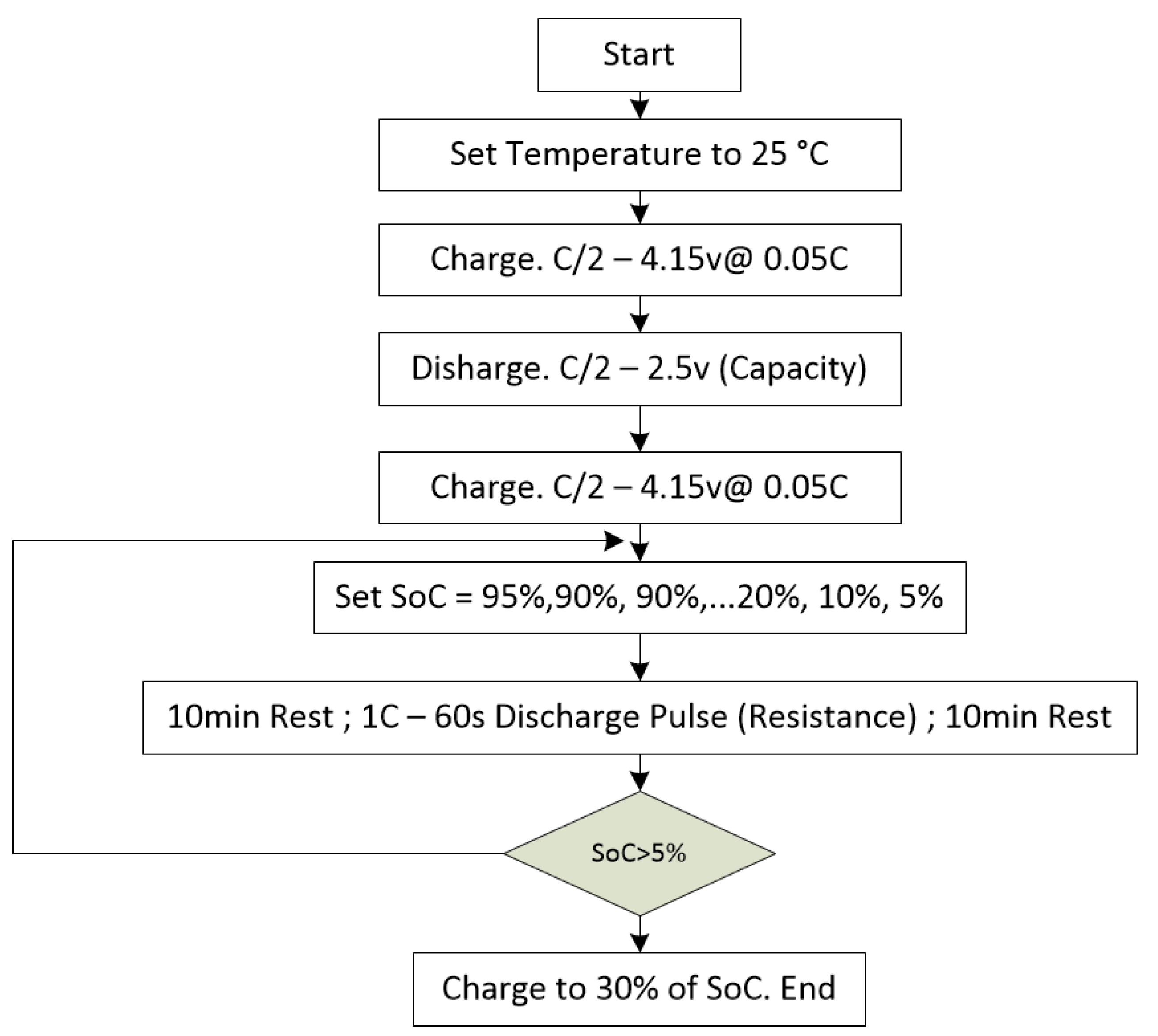
As a reference, the impedance measured during the ACT, defined in Section 2.3, is taken into consideration, which is calculated by applying a 1 C constant current rate during 60 s at 50% of SOC. The correlation between the CV step duration and the inner resistance evolution is not big enough. This time, the correlation found between these two variables presents a mean error value of 50 uOhm, evaluating numerically. As concluded in Section 4.1.1, for applications using more than one cell, this option is discarded, since the CV step could be limited by more than one cell.

4.2.2. IC Absolute and Maximum Peak Value

A similar strategy is used to check the internal impedance growth estimation, taking as reference the IC absolute and local maximum peaks. The correlation between each measured IC maximum value and the resistance is obtained by a second-order equation described in Equation (7). The parameters used in the equations (R₀, R₁ and R₂) are found using optimizations tools and minimizing the measuring and the calculated value.

$$BH{I}_{est}{}_i=R_{es{t}_i}=f\left(CPI\right)=R_{0, j}+R_{1,j }CP{I}_{j,i} +R_{2,j}CP{I}_{j,i}^2$$

(7)

Figure 9 shows the correlation of the resistance vs. different measurements. The resistance with respect to the measured maximum IC peak value is plotted in blue, the resistance vs. the local maximum value (following the strategy defined in Section 3) is in red, and the value found when the cell presents a voltage of 4 V during the charging process is shown in green. The correlation found using Equation (7) is plotted in a continuous blue line. According to the results, a mean error value of 35 uOhm is found in the case of taking into account the maximum value, 32 uOhm in the case of a local max value, and 38 uOhm using the value found at 4 V. Taking into account the initial value of the inner resistance, this means a mean absolute error of around 2%. Unlike the capacity observation, the measureable indicator with the highest correlation to the resistance seems to be the local peak value, rather than the absolute value. However, due to the similar accuracy, the maximum and local peak values can be used for resistance estimation.

4.2.3. IC Absolute and Maximum Peak Position

The second subplot from Figure 9 shows the correlation between the global and local peak position, as measured in volts with respect to the inner resistance. Again, all the data were fitted to the equation in order to evaluate the error done in the estimation of the impedance. The results obtained considering the maximum peak position are shown in blue, and the local maximum is shown in red. According to the results, mean values of 37 uOhm and 42 uOhm were found respectively for each indicator.

4.2.4. IC Modeling

Using the previously obtained information, the highest correlation between the IC curve parameters and the cell inner resistance was obtained by tracking the evolution of the local IC peak value. Figure 10 shows the relation between the impedance rise vs. the sum of A2 and A3, since they represent the local maximum value of the IC curve. According to the result, the correlation between both of the indicators is very strong, and this information can be used again to estimate the resistance of the battery in real application. Additionally, Figure 10 shows the equation that describes this correlation in a continuous red line, using the second-order polynomial definition in Equation (7). This time, compared only to all cells’ response, the mean value of the absolute error done in resistance estimation has been found to be 36 uOhm, which is less than 2% with respect to the nominal resistance of this particular cell.

5. Validation of the Algorithm at Battery Module

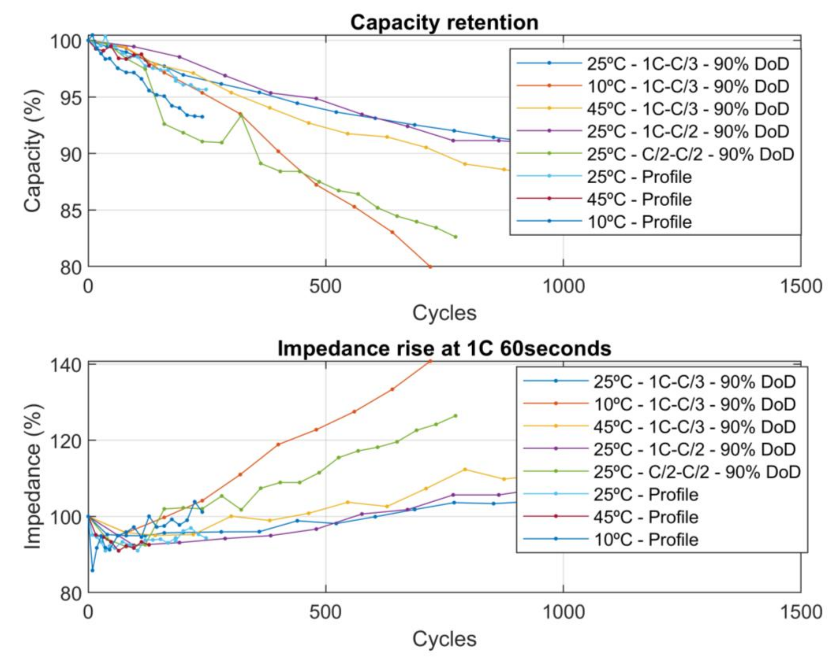
The correlation between the IC peak value and each BHI (capacity and impedance) has been investigated and validated in Section 4. Different cells have been aged at different conditions by modifying the temperature, DoD, and current. Therefore, the correlation between the IC peak value and BHI method is validated for each cell in a wide range of SOH.

In order to test the BHI estimation algorithms in a real platform, a battery module was built using the cells in a 12 series, two-parallel configuration. For measuring the cell voltage and temperature, an Analog device LTC6811 device was used with ±1 mV resolution. The value of the current through the cell was observed using a shunt resistor manufactured by Vishay, particularly using WSBS8518. The data provided by these sensors were received and processed in a TMS320f28335 microcontroller manufactured by Texas instruments. This microcontroller estimates the cell states such as state of charge, state of function, and state of health. The description and these algorithms are considered out of the scope of this work.

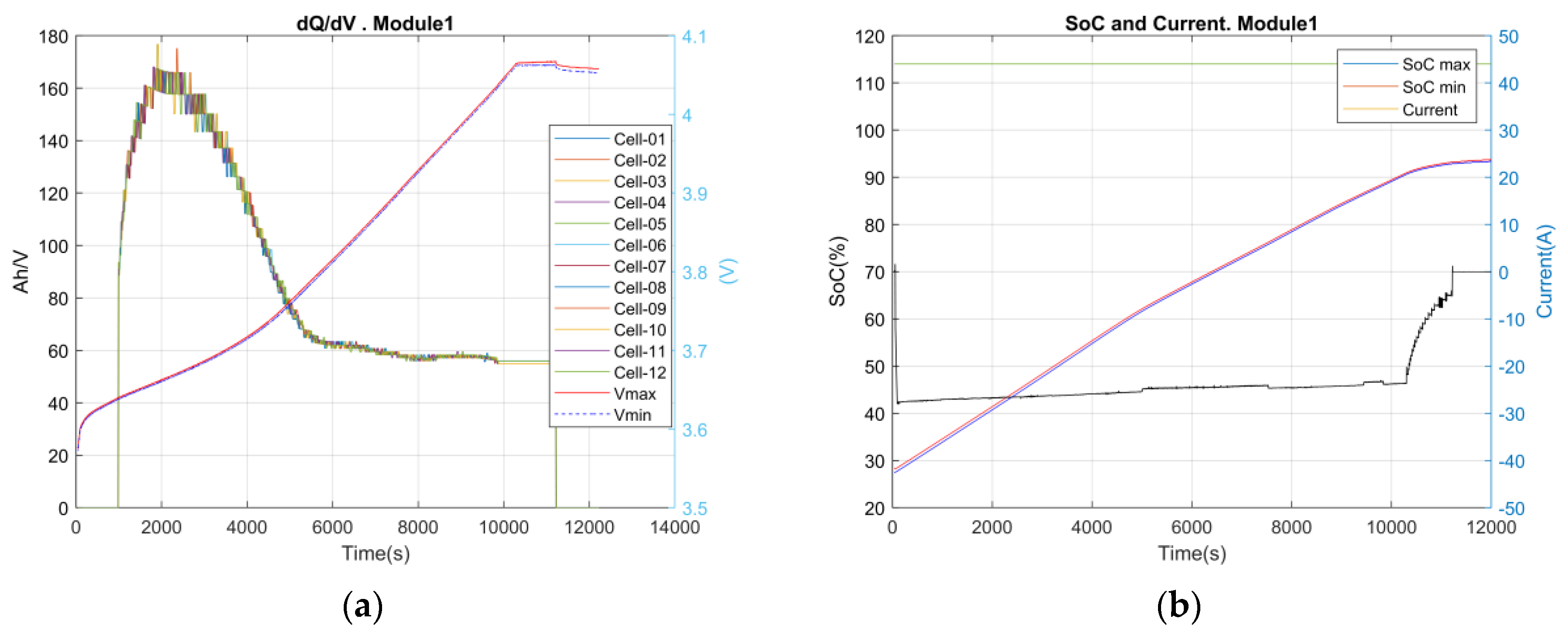
To calculate the CPI in similar conditions to a heavy-duty application, a 100 kW charger was emulated to charge a 350 kWh battery pack, scaling down the power rates to a single module level. With this energy and power ratio, the charging current rate was defined as approximately 0.3 C rate. Since the charging was done at constant power, the current presented a variation according to the voltage change. In this sense, the measured current, which is visualized in the right axis of Figure 11b, moved from 27 A at the beginning to 24 A at the end of charge.

The left side in Figure 11a shows the calculated IC curve by sampling the charging every 30 s and using a displacement of 30 between the two points used to calculate the IC. The IC calculation procedure defined in Section 3.2 has been used. In the right axis, the 12 cell voltages are visualized from 3.55 V to 4.07 V, approximately. Even though commercial elements were used to charge the module and to measure the cell variables, such as current and voltage, the IC result is very similar to the calculated one in the laboratory. In Figure 11b, the evolution of the current and state of charge of the 12 cells is visualized. The initial SOC is around 27%, and the module is charged to 95%.

By identifying the peak value of the IC curve, the values of the capacity and the resistances are calculated by processing Equations (4) and (7) and using the corresponding values of the parameters detailed in Table 4. Another alternative would be to use the graphs visualized in Figure 6 and Figure 9 for capacity and resistance, respectively. Considering a peak IC value of 160 Ah/V, the calculation of capacity gives as a result a value of 57.03 Ah (57.54 Ah measured at cell level), which is higher than the nominal value, and at the same time, it is the real capacity at the beginning of life according to the laboratory results. Regarding the resistance estimation, the result provides us with a value of 1.6 mOhm (1.55 mOhm measured at the cell level). These capacity and resistance values are in accordance with the laboratory test results, with a 0.89% and 3% error for capacity and resistance; therefore, the BHI calculation strategy is validated at the beginning of life. Further work is needed to evaluate the performance of the algorithm when the cell is aged; however, this first validation on pristine cells and the high number of degradation cases studied for the model calibration phase show the feasibility of the proposed methodology. In this sense, to reduce the testing time and maximize the results, simulation tools such as EleMA [31] can be used to test the algorithm in a controlled environment and more easily identify the potential improvements.

6. Conclusions

In this work, the correlation of different CPI and BHI have been studied and compared in order to evaluate the parameter with the highest correlation to the capacity and the impedance. According to the results, IC curve maximum value tracking can be used for estimating the battery capacity. For impedance estimation, the local maximum IC value has been concluded to be a CPI with the highest correlation to the impedance. However, the use of the peak value for impedance estimation provides similar accuracy; therefore, this CPI can be used for this purpose. The robustness of the method is checked as well in cells aged according to a test matrix, as detailed in Table 2 and initially validated in a real-life charging case for pristine cells. These low-cost computational alternatives can be applied to a set of batteries of the same batch without any need of sophisticated model-updating algorithms, such as Gaussian process, EKF, and other alternatives used in the references. In this sense, using the maximum value of the IC, a mean error of 0.56 Ah (<1%) and 35 uOhm (<2%) was found, for capacity and impedance estimation, respectively, by simply tracking the maximum values of the IC curve and applying these data to a second-order equation. Additionally, the modeling of the IC curve was implemented in order to evaluate the relation of each exponential magnitude and the capacity fade and the impedance rise. This technique presented very good results, showing a mean absolute error of 0.47 Ah and 36 uOhm for capacity and impedance, respectively. This concept presents a higher computational cost than the previous alternative, but with a higher potential to evaluate online and automatically the evolution of each degradation mechanisms, which will be considered as future research lines. Finally, the BHI estimation strategy was implemented in a real battery module and tested in a similar condition of a heavy-duty application. The results were successful, and the capacity and impedance values were aligned to the laboratory results measured at the beginning of life. Hence, the contribution of this paper is the proposal of a methodology to evaluate the optimum IC curve calculation strategy, the identification of the best CPI to estimate the BHI, the estimation of capacity and impedance, and finally, the validation of this in a real battery module.

References

1. Feng, X.; Sun, J.; Ouyang, M.; He, X.; Lu, L.; Han, X.; Fang, M.; Peng, H. Characterization of Large Format Lithium Ion Battery Exposed to Extremely High Temperature. J. Power Sources 2014, 272, 457–467. [Google Scholar] [CrossRef]
2. Birkl, C.R.; Roberts, M.R.; McTurk, E.; Bruce, P.G.; Howey, D.A. Degradation Diagnostics for Lithium Ion Cells. J. Power Sources 2017, 341, 373–386. [Google Scholar] [CrossRef]
3. Dubarry, M.; Truchot, C.; Liaw, B.Y. Cell Degradation in Commercial LiFePO4 Cells with High-Power and High-Energy Designs. J. Power Sources 2014, 258, 408–419. [Google Scholar] [CrossRef]
4. Kim, J.; Cho, B.H. State-Of-Charge Estimation and State-Of-Health Prediction of a Li-Ion Degraded Battery Based on an EKF Combined with a Per-Unit System. IEEE Trans. Veh. Technol. 2011, 60, 4249–4260. [Google Scholar] [CrossRef]
5. Plett, G.L. Extended Kalman Filtering for Battery Management Systems of LiPB-Based HEV Battery Packs: Part 3. State and Parameter Estimation. J. Power Sources 2004, 134, 277–292. [Google Scholar] [CrossRef]
6. Remmlinger, J.; Buchholz, M.; Meiler, M.; Bernreuter, P.; Dietmayer, K. State-Of-Health Monitoring of Lithium-Ion Batteries in Electric Vehicles by On-Board Internal Resistance Estimation. J. Power Sources 2011, 196, 5357–5363. [Google Scholar] [CrossRef]
7. Roscher, M.A.; Sauer, D.U.; Bohlen, O.S. Reliable State Estimation of Multicell Lithium-Ion Battery Systems. IEEE Trans. Energy Convers. 2011, 26, 737–743. [Google Scholar] [CrossRef]
8. Pop, V.; Bergveld, H.J.; Notten, P.H.L.; het Veld, J.H.G.O.; Regtien, P.P.L. Accuracy Analysis of the State-Of-Charge and Remaining Run-Time Determination for Lithium-Ion Batteries. Measurement 2009, 42, 1131–1138. [Google Scholar] [CrossRef]
9. Chen, Z.; Mi, C.C.; Fu, Y.; Xu, J.; Gong, X. Online Battery State of Health Estimation Based on Genetic Algorithm for Electric and Hybrid Vehicle Applications. J. Power Sources 2013, 240, 184–192. [Google Scholar] [CrossRef]
10. Miao, Q.; Xie, L.; Cui, H.; Liang, W.; Pecht, M. Remaining Useful Life Prediction of Lithium-Ion Battery with Unscented Particle Filter Technique. Microelectron. Reliab. 2013, 53, 805–810. [Google Scholar] [CrossRef]
11. Singh, P.; Vinjamuri, R.; Wang, X.; Reisner, D. Design and Implementation of a Fuzzy Logic-Based State-Of-Charge Meter for Li-Ion Batteries Used in Portable Defibrillators. J. Power Sources 2006, 162, 829–836. [Google Scholar] [CrossRef]
12. Hu, J.N.; Hu, J.J.; Lin, H.B.; Li, X.P.; Jiang, C.L.; Qiu, X.H.; Li, W.S. State-Of-Charge Estimation for Battery Management System Using Optimized Support Vector Machine for Regression. J. Power Sources 2014, 269, 682–693. [Google Scholar] [CrossRef]
13. Zahid, T.; Li, W. A Comparative Study Based on the Least Square Parameter Identification Method for State of Charge Estimation of a LiFePO4 Battery Pack Using Three Model-Based Algorithms for Electric Vehicles. Energies 2016, 9, 720. [Google Scholar] [CrossRef] [Green Version]
14. He, H.; Zhang, X.; Xiong, R.; Xu, Y.; Guo, H. Online Model-Based Estimation of State-Of-Charge and Open-Circuit Voltage of Lithium-Ion Batteries in Electric Vehicles. Energy 2012, 39, 310–318. [Google Scholar] [CrossRef]
15. Lu, L.; Han, X.; Li, J.; Hua, J.; Ouyang, M. A Review on the Key Issues for Lithium-Ion Battery Management in Electric Vehicles. J. Power Sources 2013, 226, 272–288. [Google Scholar] [CrossRef]
16. Hung, M.H.; Lin, C.H.; Lee, L.C.; Wang, C.M. State-Of-Charge and State-Of-Health Estimation for Lithium-Ion Batteries Based on Dynamic Impedance Technique. J. Power Sources 2014, 268, 861–873. [Google Scholar] [CrossRef]
17. Roscher, M.A.; Assfalg, J.; Bohlen, O.S. Detection of Utilizable Capacity Deterioration in Battery Systems. IEEE Trans. Veh. Technol. 2011, 60, 98–103. [Google Scholar] [CrossRef]
18. Wei, Z.; Zhao, J.; Ji, D.; Tseng, K.J. A Multi-Timescale Estimator for Battery State of Charge and Capacity Dual Estimation Based on an Online Identified Model. Appl. Energy 2017, 204, 1264–1274. [Google Scholar] [CrossRef]
19. Wei, Z.; Zhao, D.; He, H.; Cao, W.; Dong, G. A Noise-Tolerant Model Parameterization Method for Lithium-Ion Battery Management System. Appl. Energy 2020, 268, 114932. [Google Scholar] [CrossRef]
20. Yazami, R.; Reynier, Y. Thermodynamics and Crystal Structure Anomalies in Lithium-Intercalated Graphite. J. Power Sources 2006, 153, 312–318. [Google Scholar] [CrossRef]
21. Yazami, R.; Touzain, P. A Reversible Graphite-Lithium Negative Electrode for Electrochemical Generators. J. Power Sources 1983, 9, 365–371. [Google Scholar] [CrossRef]
22. Li, Y.; Abdel-Monem, M.; Gopalakrishnan, R.; Berecibar, M.; Nanini-Maury, E.; Omar, N.; van den Bossche, P.; Mierlo, J.V. A Quick On-Line State of Health Estimation Method for Li-Ion Battery with Incremental Capacity Curves Processed by Gaussian Filter. J. Power Sources 2018, 373, 40–53. [Google Scholar] [CrossRef]
23. Weng, C.; Feng, X.; Sun, J.; Peng, H. State-Of-Health Monitoring of Lithium-Ion Battery Modules and Packs via Incremental Capacity Peak Tracking. Appl. Energy 2016, 180, 360–368. [Google Scholar] [CrossRef] [Green Version]
24. Weng, C.; Cui, Y.; Sun, J.; Peng, H. On-Board State of Health Monitoring of Lithium-Ion Batteries Using Incremental Capacity Analysis with Support Vector Regression. J. Power Sources 2013, 235, 36–44. [Google Scholar] [CrossRef]
25. Li, X.; Wang, L.Y.; Zhang, Y.; Zhang, Z. A Capacity Model Based on Charging Process for State of Health Estimation of Lithium Ion Batteries. Appl. Energy 2016, 177, 537–543. [Google Scholar] [CrossRef]
26. Dubarry, M. Identifying Battery Aging Mechanisms in Large Format Li Ion Cells. J. Power Sources 2011, 196, 3420–3425. [Google Scholar] [CrossRef]
27. Dubarry, M.; Truchot, C.; Liaw, B.Y. Synthesize Battery Degradation Modes via a Diagnostic and Prognostic Model. J. Power Sources 2012, 219, 204–216. [Google Scholar] [CrossRef]
28. Dubarry, M.; Liaw, Y. Identify Capacity Fading Mechanism in a Commercial LiFePO4 Cell. J. Power Sources 2009, 194, 541–549. [Google Scholar] [CrossRef]
29. Weng, C.; Sun, J.; Peng, H. A Unified Open-Circuit-Voltage Model of Lithium-Ion Batteries for State-Of-Charge Estimation and State-Of-Health Monitoring. J. Power Sources 2014, 258, 228–237. [Google Scholar] [CrossRef]
30. Sun, Y.; Hao, X.; Pecht, M.; Zhou, Y. Remaining Useful Life Prediction for Lithium-Ion Batteries Based on an Integrated Health Indicator. Microelectron. Reliab. 2018, 88–90, 1189–1194. [Google Scholar] [CrossRef]
31. Granrath, C.; Meyer, M.A.; Andert, J.; Ewald, J.; Klink, R.; Stroh, C.; Pham, T.; Phillips, R.; Hettig, C.; Santaroni, L.; et al. EleMA: A Reference Simulation Model Architecture and Interface Standard for Modeling and Testing of Electric Vehicles. eTransportation 2020, 4, 100060. [Google Scholar] [CrossRef]
Figure 1. Capacity and impedance evolution during the lifetime of a high energy density Li-ion cell.
Energies 13 04855 g001
Figure 2. Aging check test (ACT) procedure.
Energies 13 04855 g002
Figure 3. Charging profile indicators used for estimating battery health indicators.
Energies 13 04855 g003
Figure 4. Charging profile and the incremental capacity (IC) curve calculated of one cell of the test matrix.
Energies 13 04855 g004
Figure 5. (a) Flowchart used to identify the optimum incremental capacity (IC) calculation strategy. (b) Mean and maximum error done correlating each charging profile indicators (CPI) to capacity for different displacement points N.
Energies 13 04855 g005
Figure 6. Correlation between each IC value (local peak, absolute peak, and at 4 V), position (local and absolute peak), and capacity.
Energies 13 04855 g006
Figure 7. IC curve and the evolution of the IC model parameters.
Energies 13 04855 g007
Figure 8. Correlation between parameter A4 + A5 and capacity.
Energies 13 04855 g008
Figure 9. Correlation between each IC value (local peak, absolute peak, and at 4 V), position (local and absolute peak), and the resistance.
Energies 13 04855 g009
Figure 10. Correlation between parameter A2 + A3 and resistance.
Energies 13 04855 g010
Figure 11. Charging process results. (a) dAh/dV on the left axis and the cell voltage on the right. (b) SOC on the left axis current on the right.
Energies 13 04855 g011