Article

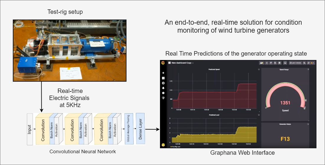
An End-to-End, Real-Time Solution for Condition Monitoring of Wind Turbine Generators

1
Department of Computer Science, University of Manchester, Manchester M13 9PL, UK
2
Department of Electrical and Electronic Engineering, University of Manchester, Manchester M1 3BB, UK
*
Author to whom correspondence should be addressed.
Energies 2020, 13(18), 4817; https://doi.org/10.3390/en13184817
Submission received: 6 August 2020 / Revised: 8 September 2020 / Accepted: 9 September 2020 / Published: 15 September 2020
(This article belongs to the Special Issue Intelligent Condition Monitoring of Wind Power Systems)

Abstract

:
Data-driven wind generator condition monitoring systems largely rely on multi-stage processing involving feature selection and extraction followed by supervised learning. These stages require expert analysis, are potentially error-prone and do not generalize well between applications. In this paper, we introduce a collection of end-to-end Convolutional Neural Networks for advanced condition monitoring of wind turbine generators. End-to-end models have the benefit of utilizing raw, unstructured signals to make predictions about the parameters of interest. This feature makes it easier to scale an existing collection of models to new predictive tasks (e.g., new failure types) since feature extracting steps are not required. These automated models achieve low Mean Squared Errors in predicting the generator operational state (40.85 for Speed and 0.0018 for Load) and high accuracy in diagnosing rotor demagnetization failures (99.67%) by utilizing only raw current signals. We show how to create, deploy and run the collection of proposed models in a real-time setting using a laptop connected to a test rig via a data acquisition card. Based on a sampling rate of 5 kHz, predictions are stored in an efficient time series database and monitored using a dynamic visualization framework. We further discuss existing options for understanding the decision process behind the predictions made by the models.

Graphical Abstract

1. Introduction

Increasingly, countries around the world seek to replace their carbon-emitting power plants with renewable sources such as wind, sunlight, tides, waves and geothermal heat. An important consideration for renewable plant operators is the maintenance of their assets which, for offshore wind turbines, has been estimated at approximately 25% of installation cost [1]. While the Levelized Cost of Electricity (LCOE) from offshore wind turbines has decreased significantly [2], newer technologies for Condition Monitoring (CM) have the potential to drive down cost. Transitioning to renewable electricity sources will not happen overnight and in the meantime some of these tools can be applicable to high-carbon sources as well as to mitigate their impact [3].
CM systems need to operate on a diverse range of wind turbines across different sites, each having its own sophisticated control system [4]. The authors describe existing data collection systems which use vibration analysis, oil particle counters, ultrasonic testing, acoustic emissions and many others. The first generation of wind turbine CM systems used for diagnostics and prognostics relied on physical explanation for operating states and failure modes [5]. These systems made assumptions of what signals to consider and how these relate to turbine operation, however, explanations for many types of failures were unavailable. Second generation CM saw an increase in statistical and machine learning techniques. Starting with data examples of failure modes, experts crafted complex pipelines of feature preprocessing and extraction (for example, using time-frequency analysis) followed by supervised machine learning models, such as Support Vector Machines (SVMs) and Decision Trees [6]. This is an error prone and time-consuming process as the pre-processing options are immense with a need for precise understanding of what works best in any given scenario. The current generation of CM models is seeing growing interest in Deep Neural Networks (DNNs). Facilitated by the computational power of GPUs, the abundance of data (Big Data), and newer initialization and training procedures, these DNNs provide end-to-end capabilities, superior performance and transferability of learned knowledge.
This aim of this paper is to show how a collection of Convolutional Neural Networks (CNNs), a type of DNN, can be trained automatically from raw current signals in an academic-scale laboratory test system representative of a type IV wind turbine generator system. Current sensors are cheap and abundant in electro-mechanical devices and the measured current data carries a large set of information relating it to operational states and fault modes. Our CNNs trained on raw currents in the time-domain accurately predict, in real-time, a set of operational state features (speed, load, magnetization level) and generalize well beyond seen examples. With up to 20 predictions/second/state, the data are stored in an open source time-series database (InfluxDB) and visualized using a dynamic interface (Grafana).
The contribution of this paper is threefold. Firstly, we showcase the applicability of CNNs to the task of predicting operational states and fault modes utilizing readily available, raw electric current data. Secondly, we discuss the details of pipeline implementation utilizing modern open source frameworks, such as Keras, for building the predictive models, i.e., InfluxDB, for storing the signals and Graphana, for interactive visualization of signals and predictions. Finally, we present several tools to assist in understanding the decisions made by the models.
This paper is organized as follows: Section 2 describes the test-rig, data sampling procedures and the models that we utilize for CM; Section 3 presents the model performance on predicting the health state, speed and load of the generator; Section 4 discusses related work, looks at the interpretability of CNN and presents an approach for efficiently storing and visualizing its outputs; Section 5 concludes and considers future work.

2. Materials and Methods

2.1. System Description

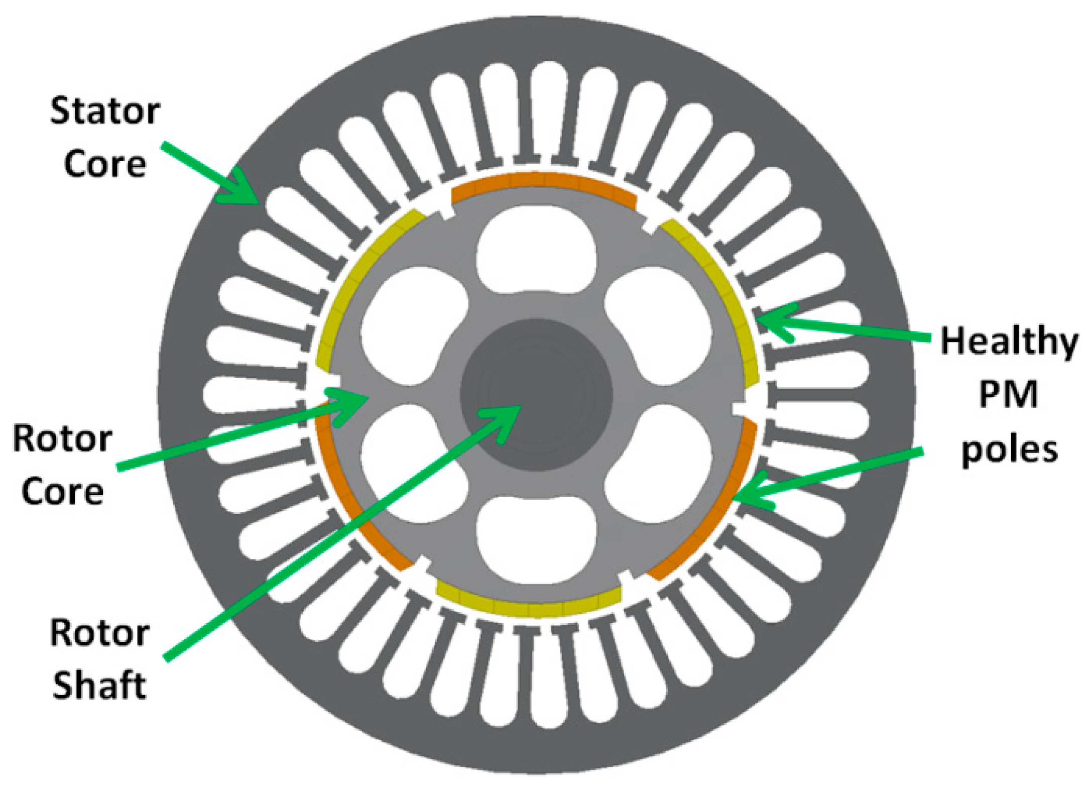
2.1.1. Examined PM Motor

This study is undertaken on a commercial 90 Hz, 415 V, 1.1 kW, 6 pole Permanent Magnet Synchronous Machine (PMSM), manufactured by LAFERT MOTORS. The rotor is a non-skewed surface mounted rotor design containing arc-shaped Permanent Magnets (PMs) of 147° ( e ) arcs, made of N-35 grade Neodymium. Figure 1 shows the cross section of the analyzed machine geometry. The original PM rotor assembly was modified to enable the emulation of a range of distinct PM magnetization conditions. The modified rotor assembly was created using the original shaft, bearings and core; however, to enable the analysis of different magnetization conditions in a controlled fashion, the original healthy PM pole arc design was modified to be circumferentially segmented into six individual sections, as can be seen in the rotor of Figure 1. This facilitates controlled emulation of a range of typical conditions that can arise from different demagnetization processes [7,8] by appropriate magnetization of individual PM sections and their careful assembly into complete PM poles to be installed on the rotor [9].

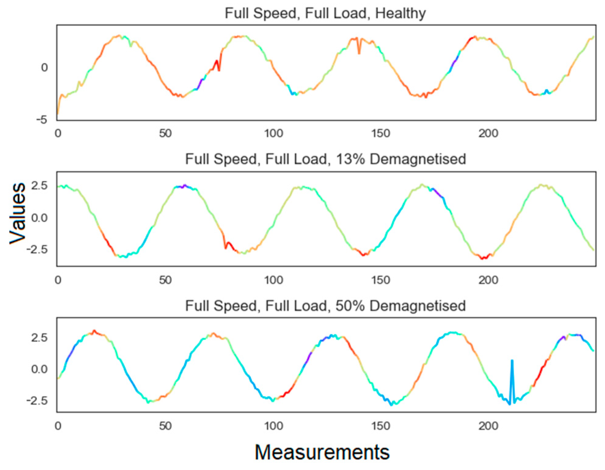
2.1.2. The Examined Demagnetized Rotor Conditions

A healthy rotor and two rotors with uniform symmetrical PM faults were prototyped for this study. The uniform demagnetization faults are manifested as identical modulation of the PM segments flux density under one pole ( B r ) [7]. To emulate this, two rotors with a symmetric ( B r ) reduction at the PM edges were prototyped. Each rotor represents a different uniform fault level: the rotors F13 and F50, corresponding to 13% and 50% of B r reduction in the leading edge of a PM pole arc, are shown in Figure 2.

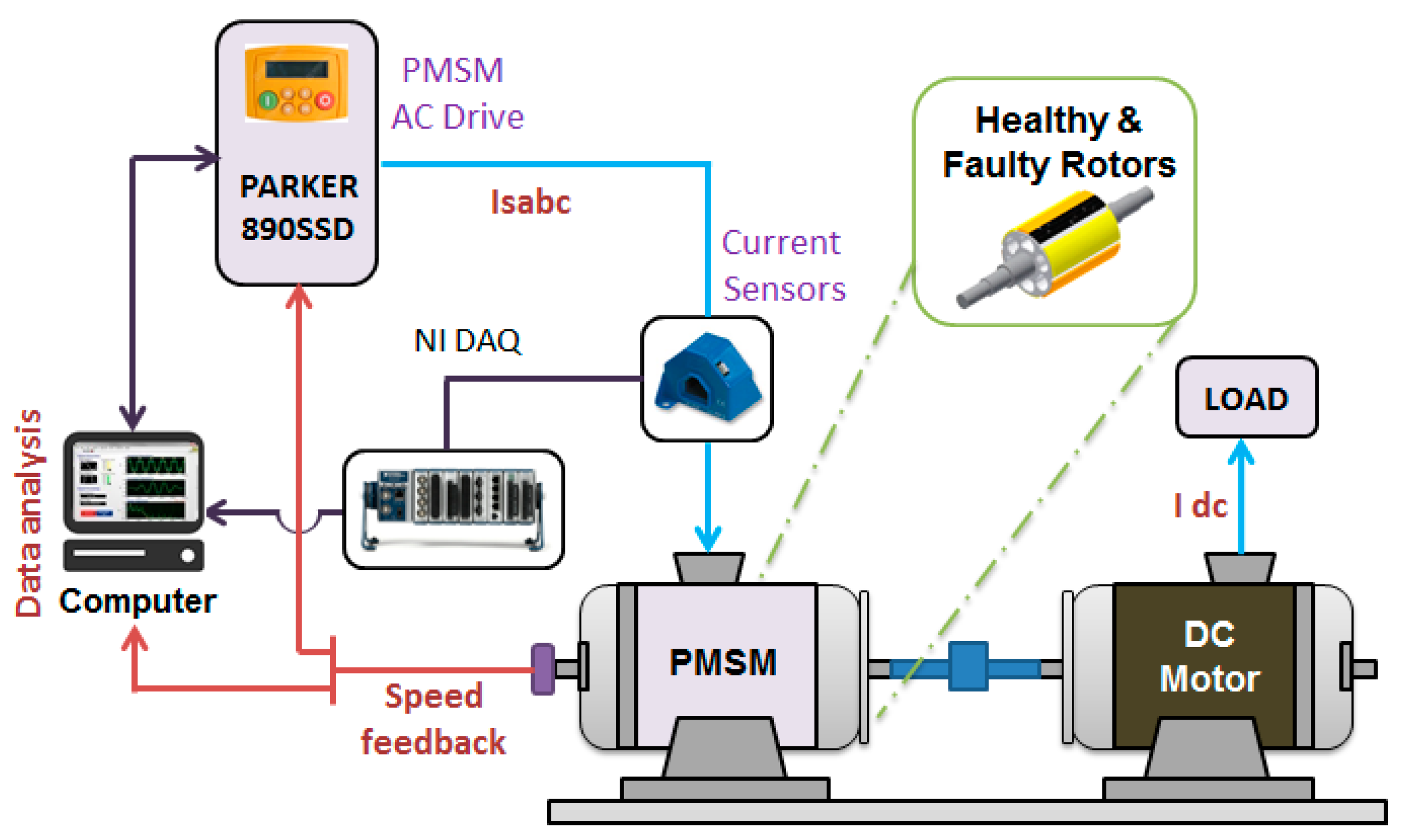
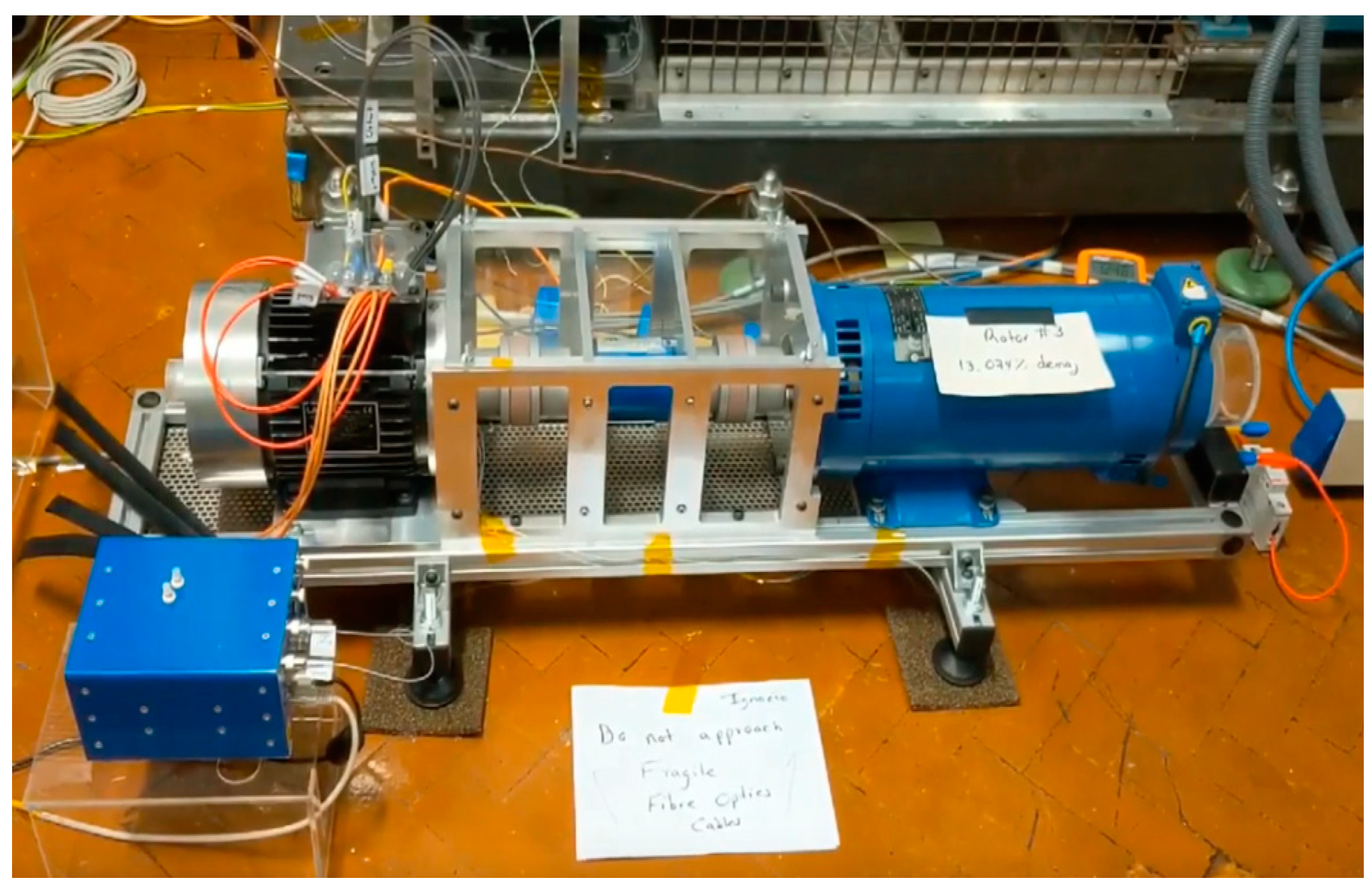
2.1.3. Test-Rig Description

The performance of the proposed algorithm was obtained from experiments on a laboratory test-rig whose configuration is shown in Figure 3 and Figure 4. A PMSM was coupled to a Direct Current (DC) motor connected to a resistor load bank. The PMSM was driven by a Parker 890SSD drive operating in Permanent Magnet Alternating Current (PMAC) vector control mode. The PMSM phase currents were sensed by LEM LA305-S current transducers connected to a NI-9205 voltage input module, mounted on a NI-compactDAQ-9178 chassis measurement system. The rotational speed of the PMSM is obtained from the resolver and sent directly to the drive feedback and computer. The PMSM can be operated using the 3 different types of rotors presented in Figure 1 and Figure 2 to emulate the healthy and faulted rotor conditions.

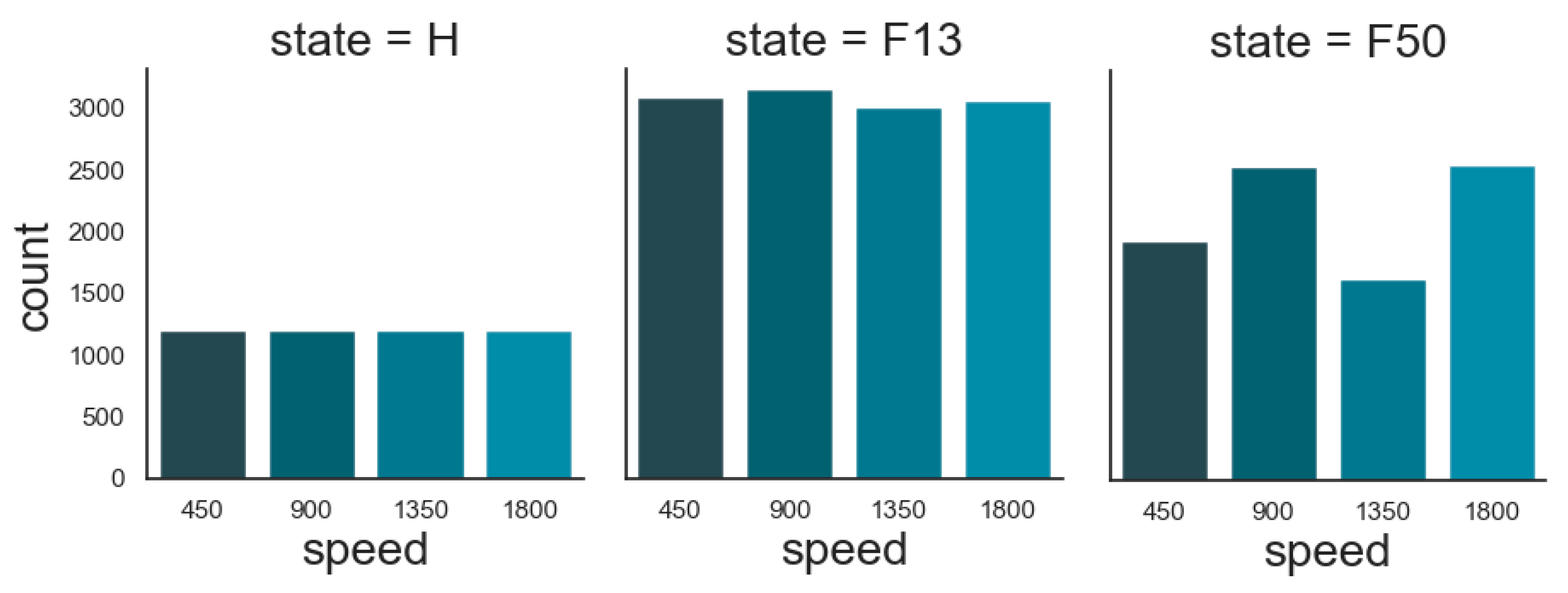
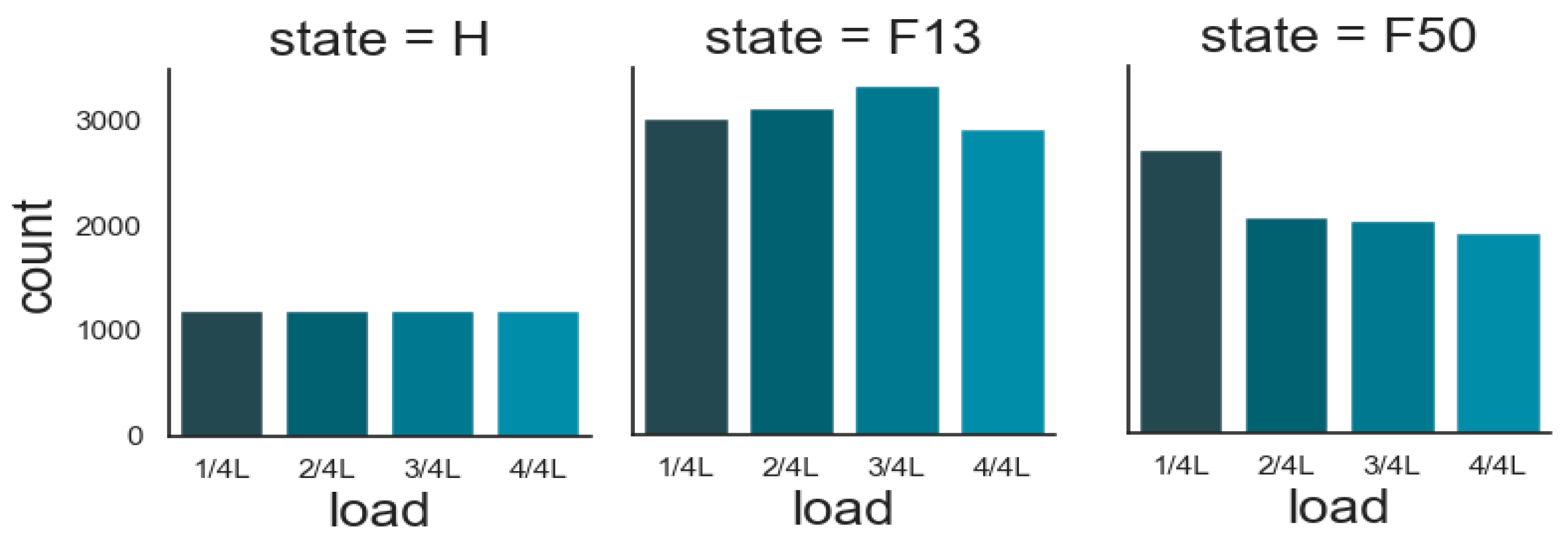
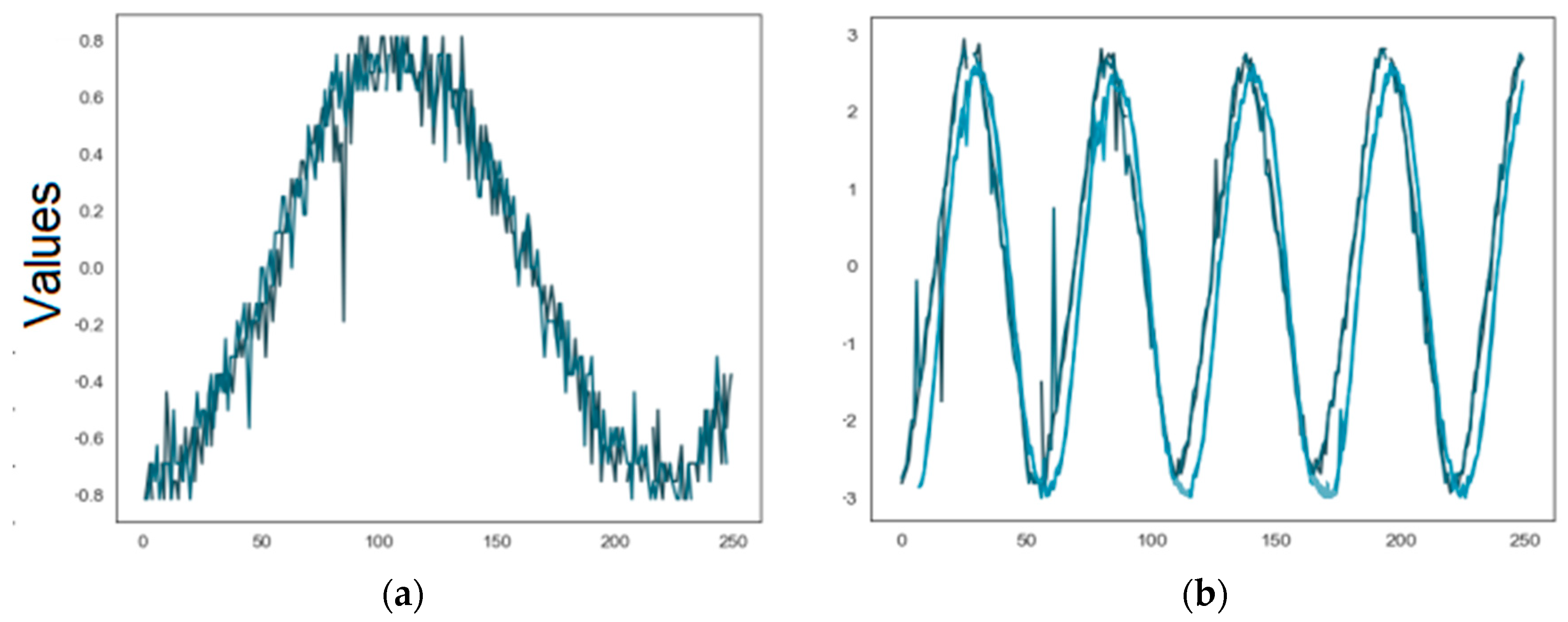
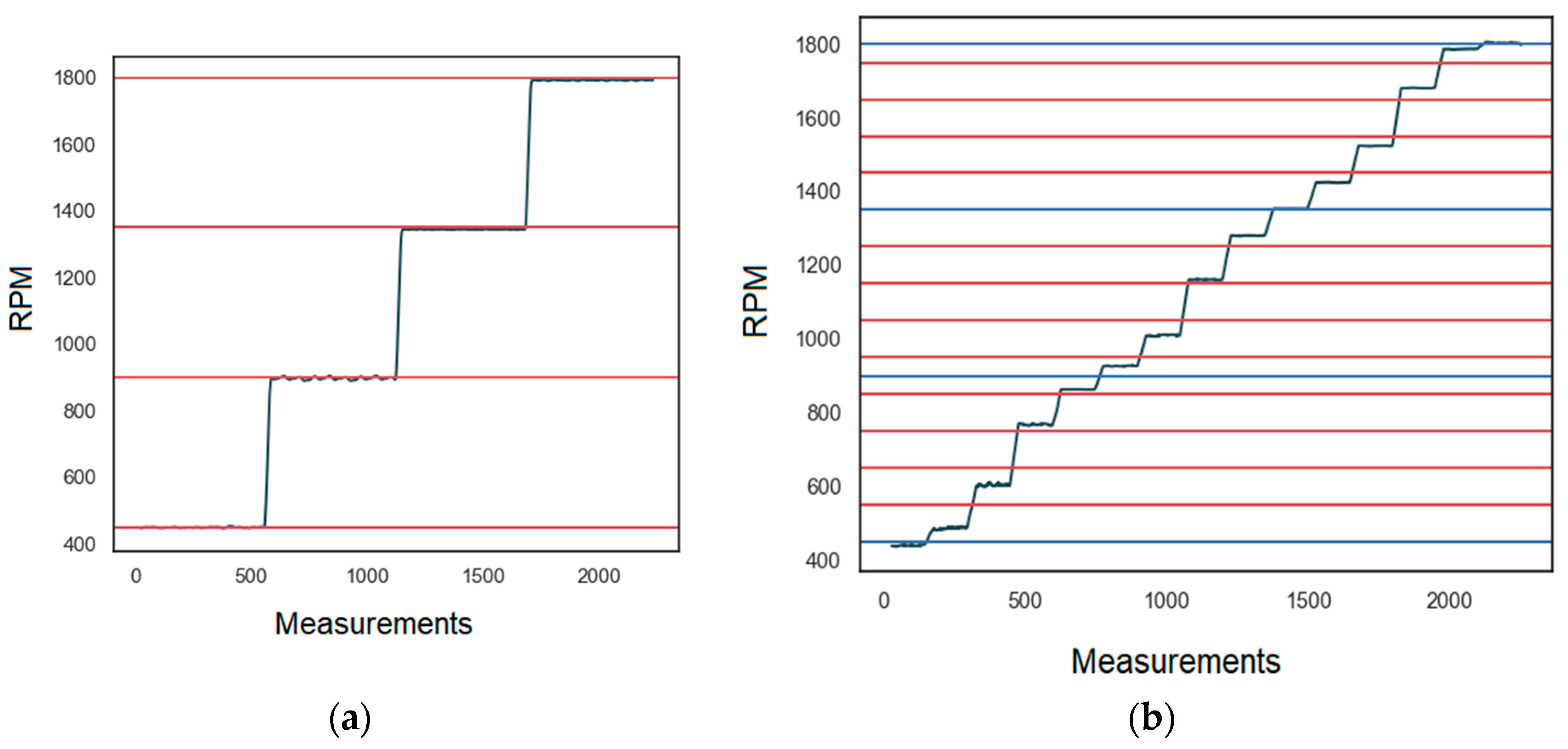
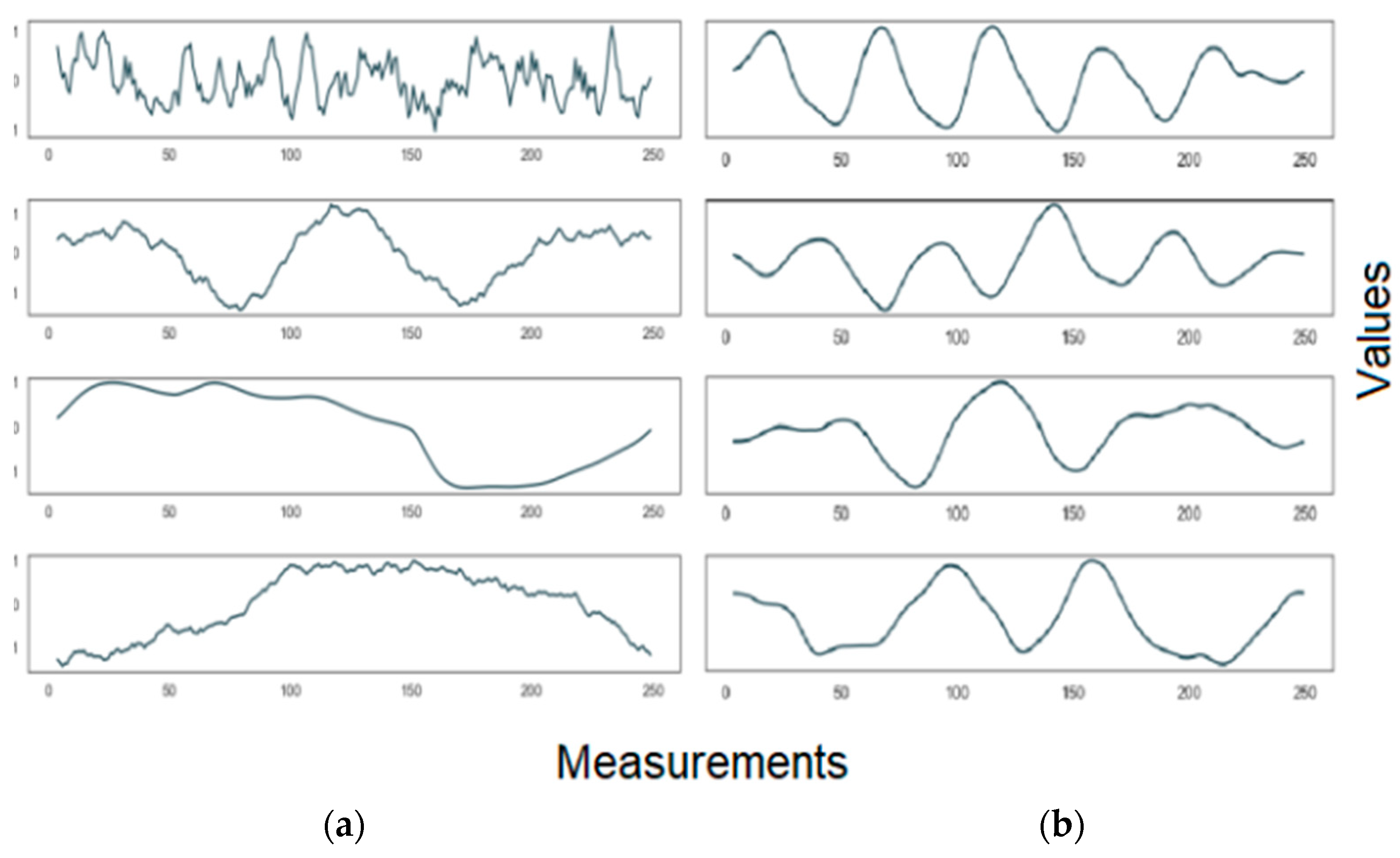
2.2. Descriptive Statistics of the Data

Using a data acquisition card (DAQ) from National Instruments, we collected currents for representing various, significant system operating states. We framed Speed and Load as continuous variables and we selected 4 equally distant points covering their whole potential state (e.g., generator speed operating range and load operating range): 1/4, 2/4, 3/4 and 4/4. For the actual examined Speed and Load conditions on the examined generator, this translates to 450 rpm, 900 rpm, 1350 rpm and 1800 rpm speeds, and 0.275 kW, 0.55 kW, 0.825 kW and 1.1 kW loads, respectively. All data were sampled at 5 kHz and split into examples containing 250 measurements, in line with findings from previous research [10] indicating this size to be a good trade-off between size and prediction accuracy. Switching through demagnetization levels makes data collection and real-time testing slower, as this requires the disassembly/assembly of the test generator and its rotor between taking measurement; while relatively time consuming due to practical work complexity constraints, this process does enable extraction of essential feature data in the time domain. We have framed the health state as a categorical variable with three states: healthy, F13 (13% demagnetization) and F50 (50% demagnetization). Figure 5 and Figure 6 show the distribution of the recorded data as a function of Speed, Load and State. Healthy data were collected first, followed by F50 and F13 cases as more data were required for accurate prediction.
Table 1 shows a case-by-case distribution of samples together with their Root Mean Squared (RMS) values. Figure 7 illustrates the differences between low vs. high speed samples. With 250 measurements we capture one current cycle at 450 rpm or four at 1800 regardless of health state. The Speed of the generator is positively correlated with the number of cycles in the electric signal, whereby increasing the former increases the latter (Figure 7). Ceteris paribus, increasing the sample size results in higher accuracies but fewer predictions per time unit. This is a logical consequence of the model receiving more data and thus increasing its chance of better predictions.
For training and validating of the models we utilized an 80/20% split of the data. Given that we use our models for diagnostic and samples are independent and identically distributed (i.i.d.) this is a valid procedure for identifying patterns in signals. If, however, models with temporal dependency (forecasting or prognostic models where the current and past data are used to predict the future) are needed, an advanced validation methodology, such as walk forward cross validation, is more appropriate [11].

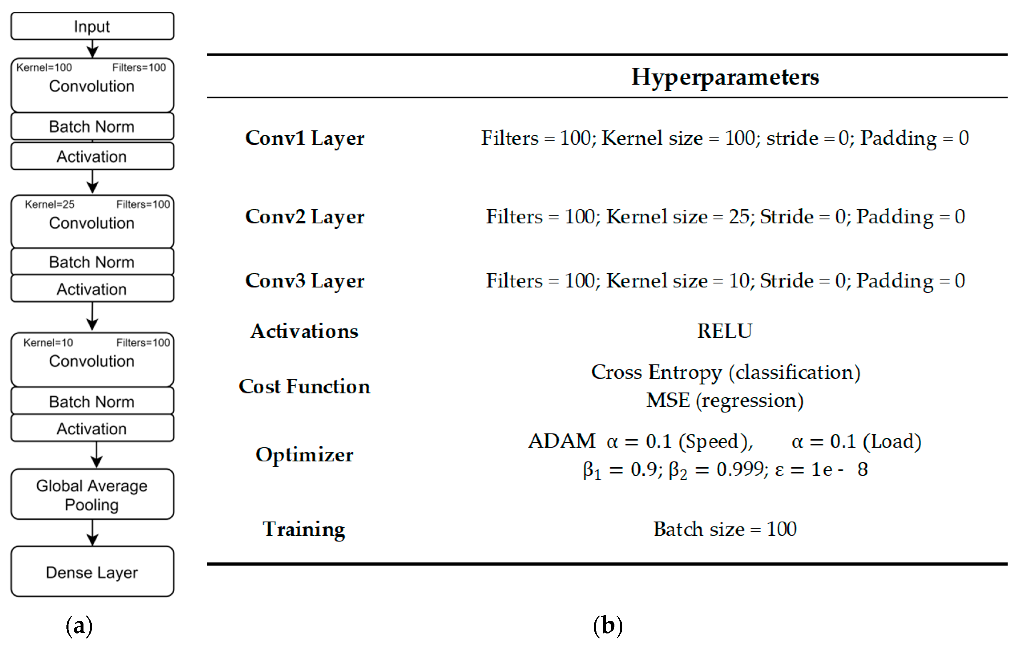
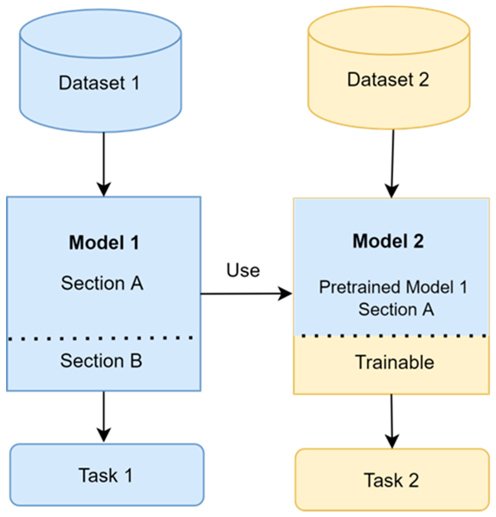
2.3. Convolutional Neural Network (CNN) Model
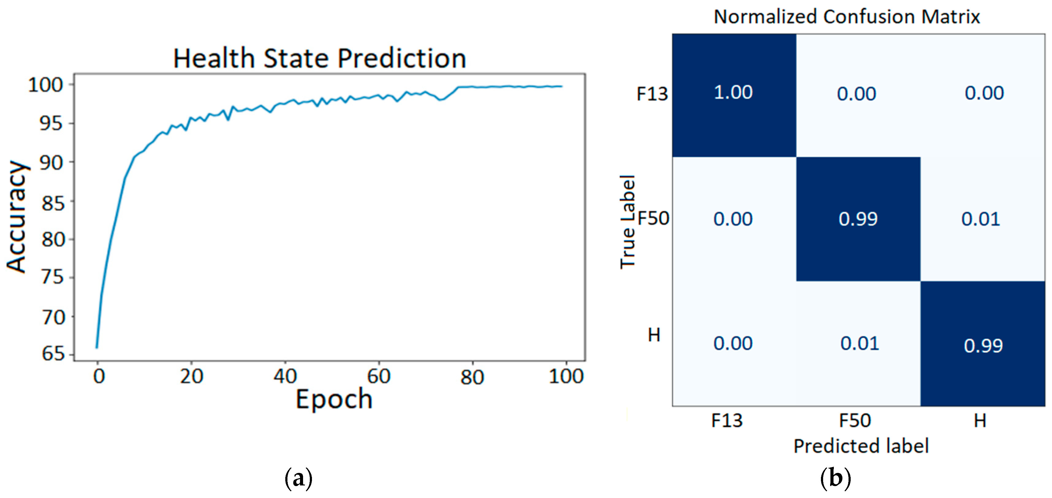
We have experimented using Keras [12] with the one-dimensional CNN architecture template described in [13], which has been shown to be a strong time series classification model over a wide range of datasets [14]. Different hyperparameters were explored, such as number of layers, filters and kernels sizes in each layer, etc.
The general architecture is made up of repeated applications of a convolution function C w ( x ) that has two operators (1): x (input) and a w (kernel to be learned); it is defined as (1) for continuous and as (2) for discrete signals:
  Cv w ( x ) =   ( x · w   ) ( t ) =   a = a = x ( a ) w ( t a ) da
Cv w ( x ) =   ( x · w   ) ( t ) =   a = a = x ( a ) w ( t a )
Each layer of a convolutional block has multiple kernels (filters) each of a predefined size (see the hyperparameters in Figure 8). The result of applying a filter is essentially performing a dot product between the input and the shifted kernel. To keep the output of the convolution the same length as the input, the latter is padded with zeros. A batch normalization BN γ β ( x ) layer is defined as:
BN γ β ( x ) = γ   x ^ + β
  x ^ =   x i μ β σ B 2 + ϵ
  σ B 2 = 1 m ( x μ B ) 2
μ B = 1 m i = 1 m x i  
where B = { x 1 x m } is the current mini-batch and γ ,   β are parameters to be learned in training. The activation function used is the Rectified Linear Unit (RELU) is defined as:
Act ( x ) =   Relu ( x ) = max ( 0 , x )
The CNN applies a series of three Conv w ,   BN γ β and Act blocks to input x as shown in Figure 8. To implement our approach, we utilized Keras which provides convolutional layer functionality for 1, 2 and 3-dimensional data. The Conv1 layer used for our models has several parameters which control the number of filters, kernel sizes, strides, padding initialization, etc. While the number of filters was kept fixed, the kernel sizes were different (see Figure 8), as this achieved better validation results on our data. Stride controls the amount that the filter moves at each step and for our purposes was set to the default of zero. We have followed each Conv1D layer with a BN layer, which in Keras is implemented as the BatchNormalization function. Its use is to normalize and scale the inputs from previous layers which in turn results in faster training and lower validation errors [15]. Using BN layers before activation layers has been shown to be successful in mitigating the internal covariant shift problem in the task of predicting faults in bearings and gearboxes [16]. Keras provides various activation functions via the Activation layer implementation: RELU, LeakyRELU, ELU, SELU, as well as the classical sigmoid and tanh. While RELU provided better results in our experiments and represents a good default it will be interesting to explore how it fares against its derivatives. A potential issue of RELU is the “dying RELU” problem which happens when the weighted sum that is fed into the activation function is less than zero resulting in a zero output and gradient, see Equation (7) and [17]. For this reason, computationally more expensive functions, such as LeakyRELU, that have a predefined slope for values less than zero, might yield better results in some settings. Keras provides implementations of several pooling functions (Max, Average, Global) over 1, 2 and 3D. This functionality downsamples the input allowing the next layers to work with smaller representations and avoid overfitting. The combination of Dense layer with Global Average Pooling in 1D (GAP) was used in our experiments as this facilitates the use of Class Activation Maps (CAMs)—discussed in Section 4.2.
Speed and Load are parameters for which we have data covering a large range of values (1/4, 2/4, 3/4 and 4/4 of their maximum). We formulated the prediction of these operating parameters as regression problems with dependent continuous variables. In addition, with more data, in the case of Speed, we can further experiment in real-time. The speed of the rig was programed a priori and was estimated using a laser tachometer and compared with our numeric predictions.
The two-regression models were trained using Mean-Squared Error (MSE) as shown in Figure 9. MSE is used to compute errors made on the training and validation sets and is defined as:
MSE   =   1 N i = 1 N (   Y ^ ( i ) Y ( i ) ) 2  
where   Y ^ ( i ) is the output of our network for input instance w and Y ( i ) is the ground truth.
The relationship between model complexity (parameters and inference times) and model performance in terms of accuracy has long been understood to be logarithmic [18]. With sustainability and explainability in mind simpler models with fewer parameters and thus lower computational complexity should be explored first (“Green AI”). Increases in the number of parameters of CNNs are justified when the function that models operational states or failures is complex and cannot be captured by the proposed architecture. Fitting the right capacitive model to the task is essential: a low capacitive model might underfit while a high capacitive model might overfit the training data. This is known as the bias/variance trade-off problem and is explained in depth in [19]. The total cost of the system grows linearly with the cost of processing a single example, the size of the training dataset and the number of hyperparameter experiments. We have also considered the strong CNN baseline architecture for time series classification proposed by Wang et al. [13] as a starting point for our models.
Learning rate α is an essential parameter of the network which controls how much weight adjustment is being made with respect to the gradients. A small value of α results in the network converging more slowly, whilst a larger value might result in the network learning more quickly but missing the local minima for non-convex functions. MSE, the cost function used in our regression, is a convex function meaning that the local minimum is also its global minima. For Speed, we used a learning rate of 0.1, while Load was 0.01. During training we have utilized ReduceLROnPlateau, a Keras callback function that is invoked when the learning process stagnates. This tool monitors the loss function and if no improvement is seen for a “patience” number of epochs (in our case 5), the learning rate is reduced by half. The “patience” is defined by the user, with the default value being 10. During our experiments, we found that choosing a patience of 5 resulted in the training converging faster to lower levels of the loss function.
We have formulated Health State prediction as a multi-class classification problem with three categorical states of the magnets. For future consideration, it is worth noting that classification can be framed as binary (one of two classes is predicted), multi-class (one of many classes is predicted), multi-label (several classes are predicted at once) or hierarchical (one class is predicted which is further divided into subclasses or grouped into super classes) [20]. In fact, magnetization is a continuous variable where any value on the spectrum between 0 and 100% may occur and a regression model for demagnetization will be considered in our future work.
To move the architecture from regression to classification we added a final dense layer with three neurons representing the potential classes. Finally, the softmax function (9) produced the outputs of the dense layer in the [0, 1] range to be used in the cross-entropy cost function computation (10):
σ j ( x ) =   e x j k = 1 9 e x k
Cos t ( x , y ) =   i = 1 9 y i log ( x i )
where x encodes the output of our network and y encodes the true class of the output. The GAP layer enables the use of Class Activation Maps (CAM) to visualize the contributing regions in the time series which lead to specific classification:
  GAP k ( x ) =   1 n x Act ( x )
where k represents the k-th filter activation in the previous layer and n represents the size of vector x.

3. Results

Model Performance

Without knowing the hyperparameters that work for a given or similar domain, fitting the best capacity deep learning model requires empirical investigation. We have experimented with different numbers of CNN blocks and hyperparameters such as filter numbers and size. Three convolution blocks of 100 filters with 100, 25 and 10 kernel sizes achieved the best results in our experiments. Different kernel sizes were used to detect smaller, medium and larger patterns. As expected, smaller networks tend to take longer (in terms of epochs) until reaching acceptable levels of MSE. For Speed prediction, we achieved an MSE of 46.61 on the training data and 40.85 on the validation set representing 20% of the data.
This result was achieved using rpm as units ranging from 450 (1/4 speed) to 1800 (4/4 of speed). The Load was trained on a range ranging from 1/4 to 4/4 and we achieved an MSE of 0.0040 (0.0018 on the validation set representing 20% of the data) after 100 epochs.
An important capability of the entire CNN-based system is to generalize the learned knowledge beyond the training cases. For this, we programmed the test-rig to run for 7 min, firstly, at different speeds seen during training—Figure 10: 450 rpm, 900 rpm, 1350 rpm, 1800 rpm levels marked in red (a)—secondly, for several unseen cases—from 450 rpm with increases of 100 rpm, up to 1800 rpm (b). While errors were close to zero in the first case, we note very small errors even for unseen cases (up to 50 rpm deviation from actual). The deviations tend to have higher volatilities for lower speeds which tend to be more challenging to address, as the samples contain less information (fewer electric cycles) (Figure 10b).
With the Cross-entropy function (Equation (10)) as a cost function in the architecture and hyperparameters set as in Figure 8, the CNN trains for 100 epochs reaching 99.67% accuracy on the validation set representing 20% of data (Figure 11a). As a function of the number of epochs, the accuracy follows the rule of diminishing returns with the highest levels plateauing after 100 epochs (a sign that the training has reached the local minima of the cost function). These validation data are set aside at the beginning of the experiment.
Supervised classification algorithms are often presented with confusion matrices to help understand on which classes the model makes errors and/or where it is most accurate. Here (Figure 11b), we observe that the network successfully identifies the F13 case (100% accurate) with 0.34% of the errors being made on the F50 and Healthy cases.

4. Discussion

To our knowledge, this is the first paper that presents an operational and highly accurate working prototype trained in an end-to-end approach, with real-time capability and efficient storage and monitoring of predicted diagnostics.

4.1. Related Work

Recent algorithmic developments, allied to availability of data and increased computing power, suggest that deep learning is the most advanced technique for pattern recognition [19]. Being able to stack hundreds of layers of neurons has expanded the range of complex functions that can be learned from a variety of structured and unstructured data. Fawaz et al. [21], provides a detailed account on existing end-to-end time series architectures that utilize deep learning for prediction.
These approaches have begun to be adapted for machine health monitoring models (Zhao et al., [5]). The authors explain that machine learning models for diagnostics fall into three categories:
  • Traditional physics-based models: these models assume a mathematical understanding behind failures and are rigid in updating with new data;
  • Conventional data-driven models: bottom-up approaches that offer more flexibility but are unable to model large scale data; such models require expert knowledge and hand-crafted features;
  • Deep-learning models: a bottom-up approach based on Artificial Neural Networks (ANNs), which find discriminating features in data without the need for an expert and represent a stepping stone towards end-to-end learning.
Hence, deep learning offers significant potential for more timely, accurate and economical diagnostics to achieve a lower maintenance cost which is essential for the adoption of renewables.
Ince et al. [22] describe work using CNNs for real-time motor fault detection. They developed an elegant and flexible solution which combines feature extraction and classification at a low computational cost using a CNN. From a Three-Phase Squirrel Cage Induction Motor, they obtained 2600 of healthy and 2600 of faulty bearing samples. Their model consists of three hidden convolution layers and two deep Multilayer Perceptron (MLP) layers. These CNN-based results are competitive in comparison to complex models requiring preprocessing using Fourier or Wavelet Packet Transforms, in terms of accuracy (97.4%), sensitivity (97.8%), specificity (97.0%) and positive prediction (97.0%).
Wang et al. [13] introduced an end-to-end CNN model for time series classification that claimed state-of-the-art performance on 44 time series datasets from the University of California Riverside (UCR) archive [14]. Their CNN architecture achieved lower Mean Per-Class Error than approaches such as MLPs, ResNet, Multi-Scale CNN (MCNN) and several others. To interpret the decision making behind their CNN model, the authors [13] used Class Activation Maps (CAMs) to identify the contributing regions in the raw time domain. This uses the Global Average Pooling Layers, which also reduce the number of parameters and improves generalization. With previous claims of state-of-the-art performance on univariate time series classification, MCNN [23] has seen recent successes in CM of rolling bearing in shipborne antennas [24]. The drawback of MCNN is the need for additional data-preparation operations such as down-sampling, smoothing, sliding windows, etc., which requires expert intervention.
Sun et al. [25] proposed a CNN and SVM to diagnose motor faults using vibration signals. The model accurately distinguishes (97.8 to 100%) between six motor conditions: normal, stator winding defect, unbalanced rotor, defective bearing, broken bar, bowed rotor. However, as well as introducing the complexity of new parameters for the SVM (choice of kernel function, C-penalty parameter, degree of the polynomial kernel, etc.), vibration signals have been identified as potentially unreliable.
Kao et al. [26] showed that vibration signals often encounter problems related to noise that cannot be fully suppressed and influence diagnostic accuracy. To address these issues, the authors proposed a CNN mode utilizing stator current to predict five different motor states, including two different demagnetization fault states and two bearing fault states. Further, varying the speed between 150 and 3000 rpm results in more discriminative features being selected. Using CNN achieves better performance (98.8%) compared with a Wavelet-packet transform model (98.1%), a traditional methodology requiring expert hyperparameter tuning (e.g., mother function, number of features, etc.).
Jeong et al. [27] trained a CNN to predict demagnetization faults and inter-turn short circuits for Interior Permanent Magnet Synchronous Machines (IPMSMs). Using stator currents, the authors extracted nine components of the Fourier Transform which were used with a shallow, two-layer CNN. The authors report 99.87% accuracy for the training set and 98.96% on the test set. For demagnetization fault prediction, they identify a fundamental component much larger than normally explained by current flow due to the back electromotive force. As was shown with our procedure, a deeper CNN is able to extract the relevant features without the use of the intermediate step of Fourier Transform.
A normal behavior model was proposed by Kong et al. [28] that uses both a CNN and a Gated Recurrent Unit (a type of RNN). This fused model was trained on a healthy Supervisory Control and Data Acquisition (SCADA) dataset which allows for residual analysis when functioning in real-time. At each time t, m features are produced by convolving SCADA sensor data with a filter of size one, extracting spatial features. These spatial features are then fed into an autoregressive Gated Recurrent Unit (GRU) model that predicts future values for each sensor. Predicted values are compared to real ones and deviations indicate departure from the healthy state. The authors showcase their approach on a use case involving gear crack and compare their method positively to several others.
Given that ANNs come in many types of architecture (e.g., Multi-Layer Perceptrons or MLPs, CNN, Recurrent Neural Networks (RNN), Transformers, etc.) the selection of the right approach for a given problem is challenging. Compounding this problem is the fact that they are generally flexible enough to make relatively good predictions even for wrong input data. MLPs with non-linear activations have been shown, through the universal approximation theorem, to be able to represent any function with small error [29]. In classification problems where there is spatial (e.g., neighborhood pixels in 2D images) or sequential relatedness (as in univariate or multivariate signals), CNNs represent an appropriate choice. A major benefit from using CNNs is their sparse interaction with kernels that are much smaller than the input which makes them more efficient, with fewer parameters needed and a lower memory footprint [19]. The convolution operation results in outputs which are a function of relatively small neighborhoods predefined by the user in convolution layer kernel sizes.
For our diagnostic task, we have used CNN as it can capture the neighboring measurement relationship when point-predictions are made on real-time samples (our models see the smallest, last batch of measurements).
When longer term temporal dependencies between measurements are expected and the task is to predict the system’s future state (as in prognostics), RNN variants might become more relevant. Unlike CNNs, which share parameters in kernels, RNNs make use of internal memory states which are passed between consecutive computations. RNNs, such as the Gated Recurrent Unit (GRU) and Long Short-Term Memory (LSTM), have been successfully used in other sequence prediction problems in domains ranging from natural language modelling [30], to physics [31], speech recognition [32] and so on. A requirement of RNNs is that sequential data are processed in an order that limits their parallelization. A more recent architecture called Transformer [33] overcomes this limitation achieving state-of-the-art results on Natural Language Processing (NLP) tasks with potential for time series forecasting [34]. This architecture will be investigated in the future.
A major benefit from using models, such as CNN, is their powerful hierarchical representation of learned features. While the initial layers capture small patterns and variations in the input signals, the complexity of the learned features increases as a function of network depth. Transfer learning is about reusing lower layers of a pretrained model (Model 1 Section A in Figure 12) to speed up the training of a second model (Model 2 in Figure 12) on a related task. In some cases, the training time can be effectively reduced by a factor of 4 as in [35]. Future work will investigate the reuse of weights via transfer learning for the task of predicting failures.

4.2. Interpreting CNN Results

An argument against deep learning is lack of interpretability. Unlike decision trees, which have self-explainable, tree-like decision structure, the patterns learned by CNNs are encoded in synaptic weights which are stored as a matrix of floats. Using backpropagation, these weights are adjusted during training in such a way as to minimize our cost function of choice (e.g., MSE).
While model agnostic methods (e.g., partial dependence plots) are generally applicable [36], special tools have been developed to aid interpretation. The layers of a CNN learn increasingly complex features as a function of depth and in order to visualize these features one can optimize:
t s * = a r g m a x t s 1 n i = 1 n a c t L ( t s )
where ts can be a time series representing a sample, then optimization essentially selects the sample which maximizes the activations in layer L.
While this is a valid approach, it does not work well when multiple elements are present at the same time yielding mixed features. The solution here was to start with an empty series of 250 measurements (same size as our sample data), which was tweaked through multiple iterations so as to maximize sum ( a c t L ). Finally, we have 100 maximized activations, one for each convolution filter; an effective way to summarize and plot them is by clustering into four groups (using K-means [37])—see Figure 13 which presents the first (a) and last activation (b) layers of the model trained to predict generator speed. As expected, increasing feature complexity illustrates the hierarchical nature of feature learning in convolutional networks. The shapes of the series in Figure 13b show patterns that are intuitive to understanding of speed: some filters are activated when a sample has more cycles (high speed) or fewer cycles (low speed).
Another tool of note is Class Activation Maps (CAMs), which show which segments in the time domain cause the network to make specific classifications. The equations describing CAMs are:
  g k =   k w k c x S k ( x ) =   k x w k c S k ( x )
  M c = k w k c S k ( x )
where S k ( x ) represents the k-th filter activation in the last convolutional layer at temporal location x and w k c represents the weight of the final softmax function for the output from filter k and class c.
Figure 14 shows the parts of the signal that the CNN finds to be relevant for predicting the State as healthy—13 and 50% demagnetized at high speeds and high loads. We illustrate this by coloring in red the discriminative segments and in blue the ones that the network thinks are irrelevant. The CNN considers larger, uniform segments in the time domain to confidently predict the healthy case, valleys for the 13% demagnetized case and peaks and valleys for the 50% demagnetized current.

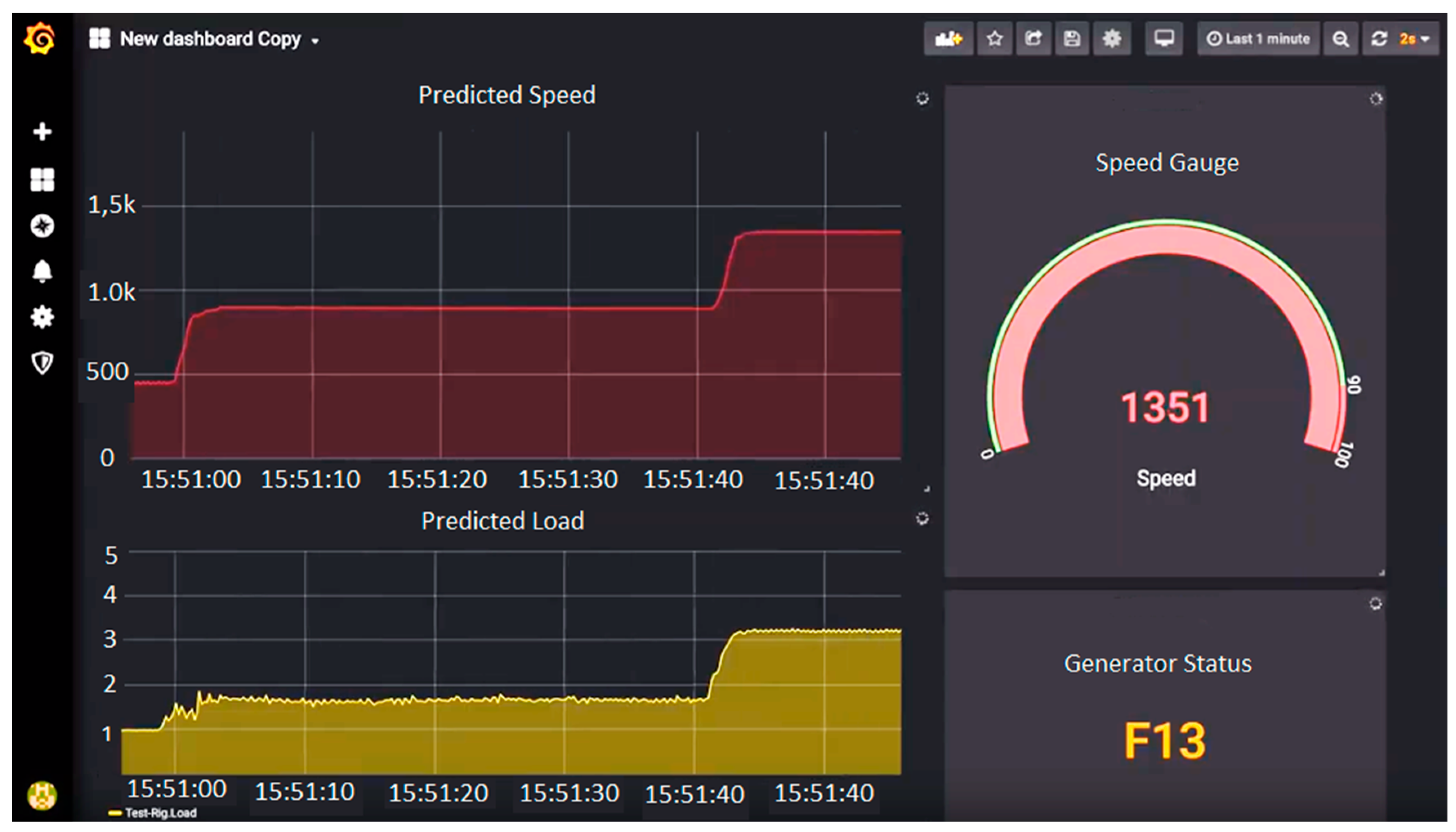
4.3. Storage and Visualization

To gather data, we utilize NI-DAQmx [38] which is a Python API for interacting with the National Instruments Data Acquisition Cards. For developing the CNNs, we utilize Keras API [12] which provides a layer of abstraction above TensorFlow [39]. Knowledge of TensorFlow is particularly useful if finer control of the underlying models is needed.
Once the models have been trained, with the laptop connected to the test-rig, a callback function is called 20 times per second requesting the CNNs to predict speed, load and health state. The results are packed into a JSON document and sent to an InfluxDB [40], an open source, Time-Series Optimized Database (TSDB). Compared to traditional database systems, TSDBs have fast and easy range queries, high writing performance, data co-location, data compression, scalability and usability [41]. As of August 2019, InfluxDB dominates the ranking of DB-Engines [42] which collects monthly information about usage of database management systems. We further utilize Grafana [43], an open source analytics and monitoring platform, to monitor the predictions made by our CNNs in real-time.
To visualize predictions, we utilize Grafana [43]. Grafana can connect to various DBs natively providing specific query editors. It supports time series plots, heatmaps, histograms, geomaps and many other tools which aid in understanding data. In Figure 15, we present a screenshot of Grafana’s dashboard showing Speed and Load as time series plots—Speed as a gauge, Health Status as a Text Box. Of relevance for diagnostics and maintenance is Grafana’s alerts system, which can be set visually using the dashboard. Criteria such as “Speed > threshold in the last hour” can trigger alerts with custom messages being sent via email, Slack, PagerDuty, etc.

5. Conclusions

Before its universal adoption, renewable energy has various hurdles to cross, such as intermittency, variable capacity and the high cost of maintenance. This study provides requirements for and analyzes the efficacy of establishing an autonomous deep learning application for CM of a Type IV permanent magnet wind turbine generator. The paper further describes an end-to-end, real time set of models for system diagnostics, an integral part of operation and maintenance.
We have shown how to create a complete and functional diagnostic system from a fundamental level, starting with test-rig hardware setup, data acquisition, end-to-end model training and validation, real-time operation, efficient signal storage and interactive visualization. Moreover, the system only relies on raw current signals which are readily available, cost effective to monitor and usually already captured in commercial wind turbine systems for control purposes.
Using a purpose-built Type IV wind turbine generator test rig, we sampled currents at 5 kHz representing different levels of speed, load and health state (magnetization). Splitting into examples of 250 measurements allowed us to train models to make 20 predictions per second, a rate which can theoretically increase with higher sampling rates. Given the continuous range of generator speed and load, we sampled uniformly four equidistant points in their operating range for training data selection. Cast as a regression problem, both models achieved low MSE (x and y). We have shown that the speed model can predict and generalize well beyond the specific ranges on which it was trained.
Deep Learning with CNNs has been used with MSE (Speed and Load) and Cross-Entropy (Health State) as cost functions. Compared to traditional data-driven approaches that require feature engineering, these models combine multiple feature extraction stages with a classifier resulting in end-to-end architectures that run on raw data. This represents a paradigm shift from time-consuming, error-prone feature processing of raw signals.
Utilizing Class Activation Maps enables visualization of segments in the time domain which triggers the models to predict classification decisions. This has the potential to guide and inform a physics-based understanding of the relation between signals and fault states. Connected to the test-rig our system makes 20 predictions per second in real time, stores them in an efficient time-series oriented database (InfluxDB) and interactively visualizes them using Grafana.
Future work will expand the collection of models to include other operational and fault states. We will extend the work on magnetization and frame it as a regression problem aiming to predict arbitrary levels of demagnetization. Moreover, we will consider non-uniform demagnetization where magnets fail arbitrarily around the shaft. Further, we are interested in exploring diagnostics for other types of failures, such as those occurring in bearings. For faults that cannot be reliably predicted using sensed currents alone, we are interested in sensor data fusion and multivariate CNNs.

Author Contributions

Conceptualization, A.S., J.M.R., S.D., A.M. and G.N.; methodology, A.S., J.M.R., A.M. and S.D.; software, A.S.; validation, A.S. and J.M.R.; investigation, G.N. and J.K.; resources, S.D., servers: G.N., J.K.; data curation, A.S.; writing—original draft preparation, A.S.; writing—review and editing, J.K.; visualization, A.S.; supervision, G.N.; project administration, G.N. and S.D.; funding acquisition, G.N. All authors have read and agreed to the published version of the manuscript.

Funding

This research was funded by the Engineering and Physical Sciences Research Council (EPSRC) grant numbers EP/P009743/1 and EP/L021463/1.

Acknowledgments

The authors are thankful to all colleagues and partners on the HOME Offshore project (http://homeoffshore.org/). The data used in this study can be made available upon request.

Conflicts of Interest

The authors declare no conflict of interest.

References

  1. Barnes, M.; Brown, K.; Carmona, J.; Cevasco, D.; Collu, M.; Crabtree, C.; Crowther, W.; Djurovic, S.; Flynn, D.; Green, P.R.; et al. Technology Drivers in Windfarm Asset Management Position Paper. 14 June 2018. Available online: https://www.windpoweroffshore.com/article/1448667/uk-offshore-facing- (accessed on 31 August 2020).
  2. Orsted. Making Green Energy Affordable How the Offshore Wind Energy Industry Matured-and What We Can Learn from it. Available online: orsted.com/en/about-us/whitepapers/making-green-energy-affordable (accessed on 1 September 2020).
  3. Rolnick, D.; Donti, P.L.; Kaack, L.H.; Kochanski, K.; Lacoste, A.; Sankaran, K.; Ross, A.S.; Milojevic-Dupont, N.; Jaques, N.; Waldman-Brown, A.; et al. Tackling Climate Change with Machine Learning. 2019. Available online: http://arxiv.org/abs/1906.05433 (accessed on 1 September 2020).
  4. Yang, W.; Tavner, P.J.; Crabtree, C.J.; Feng, Y.; Qiu, Y. Wind turbine condition monitoring: Technical and commercial challenges. Wind Energy 2014, 17, 657–669. [Google Scholar] [CrossRef] [Green Version]
  5. Zhao, R.; Yan, R.; Chen, Z.; Mao, K.; Wang, P.; Gao, R.X. Deep Learning and Its Applications to Machine Health Monitoring: A Survey. Mech. Syst. Signal Process. 2015, 14, 1–14. [Google Scholar] [CrossRef]
  6. Stetco, A.; Dinmohammadi, F.; Zhao, X.; Robu, V.; Flynn, D.; Barnes, M.; Keane, J.; Nenadic, G. Machine learning methods for wind turbine condition monitoring: A review. Renew. Energy 2019, 133, 620–635. [Google Scholar] [CrossRef]
  7. Melecio, J.I.; Djurović, S.; Schofield, N. FEA model study of spectral signature patterns of PM demagnetisation faults in synchronous PM machines. J. Eng. 2019, 2019, 4127–4132. [Google Scholar] [CrossRef]
  8. Mohammed, A.; Melecio, J.I.; Djurović, S. Electrical Machine Permanent Magnets Health Monitoring and Diagnosis Using an Air-Gap Magnetic Sensor. IEEE Sens. J. 2020, 20, 5251–5259. [Google Scholar] [CrossRef]
  9. Melecio, J.I.; Mohammed, A.; Djurovic, S.; Schofield, N. 3D-printed rapid prototype rigs for surface mounted PM rotor controlled segment magnetisation and assembly. In Proceedings of the 2019 IEEE International Electric Machines and Drives Conference (IEMDC 2019), San Diego, CA, USA, 11–15 May 2019. [Google Scholar]
  10. Stetco, A.; Mohammed, A.; Djurovic, S.; Nenadic, G.; Keane, J. Wind Turbine operational state prediction: Towards featureless, end-to-end predictive maintenance. In Proceedings of the 2019 IEEE International Conference on Big Data (Big Data), Los Angeles, CA, USA, 9–12 December 2019; pp. 4422–4430. [Google Scholar]
  11. De Prado, M.L. Advances in Financial Machine Learning, 1st ed.; Wiley Publishing: Hoboken, NJ, USA, 2018. [Google Scholar]
  12. Chollet, F. Keras. 2015. Available online: https://keras.io (accessed on 1 September 2020).
  13. Wang, Z.; Yan, W.; Oates, T. Time series classification from scratch with deep neural networks: A strong baseline. arXiv 2017, arXiv:1611.06455v4. [Google Scholar]
  14. Chen, Y.; Keogh, E.; Hu, B.; Begum, N.; Bagnall, A.; Mueen, A.; Batista, G. The UCR Time Series Classification Archive. 2015. Available online: https://www.cs.ucr.edu/~eamonn/time_series_data/ (accessed on 31 October 2018).
  15. Ioffe, S.; Szegedy, C. Batch normalization: Accelerating deep network training by reducing internal covariate shift. arXiv 2015, arXiv:1502.03167. [Google Scholar]
  16. Wang, J.; Li, S.; An, Z.; Jiang, X.; Qian, W.; Ji, S. Batch-normalized deep neural networks for achieving fast intelligent fault diagnosis of machines. Neurocomputing 2019, 329, 53–65. [Google Scholar] [CrossRef]
  17. Géron, A. Hands-on Machine Learning with Scikit-Learn and Tensor Flow: Concepts, Tools, and Techniques to Build Intelligent Systems; O’Reilly Media: Sebastopol, CA, USA, 2019. [Google Scholar]
  18. Ai, G.; Dodge, J.; Smith, N.A.; Etzioni, O.; Ai, R. Green AI. 2019. Available online: https://arxiv.org/abs/1907.10597 (accessed on 31 August 2020).
  19. Goodfellow, I.; Bengio, Y.; Courville, A. Deep Learning; MIT Press: Cambridge, MA, US, 2016. [Google Scholar]
  20. Sokolova, M.; Lapalme, G. A systematic analysis of performance measures for classification tasks. Inf. Process. Manag. 2009, 45, 427–437. [Google Scholar] [CrossRef]
  21. Fawaz, H.I.; Forestier, G.; Weber, J.; Idoumghar, L.; Muller, P.-A. Deep learning for time series classification: A review. Data Min. Knowl. Discov. 2019, 33, 917–963. [Google Scholar] [CrossRef] [Green Version]
  22. Ince, T.; Kiranyaz, S.; Member, S.; Eren, L. Real-Time Motor Fault Detection by 1-D Convolutional Neural Networks. IEEE Trans. Ind. Electron. 2016, 63, 7067–7075. [Google Scholar] [CrossRef]
  23. Cui, Z.; Chen, W.; Chen, Y. Multi-Scale Convolutional Neural Networks for Time Series Classification General Terms. Available online: https://arxiv.org/pdf/1603.06995.pdf (accessed on 16 July 2019).
  24. Pan, T.; Chen, J.; Zhou, Z.; Wang, C.; He, S. A Novel Deep Learning Network via Multi-Scale Inner Product with Locally Connected Feature Extraction for Intelligent Fault Detection. IEEE Trans. Ind. Inform. 2019, 15, 5119–5128. [Google Scholar] [CrossRef]
  25. Sun, W.; Zhao, R.; Yan, R.; Shao, S.; Chen, X. Convolutional Discriminative Feature Learning for Induction Motor Fault Diagnosis. IEEE Trans. Ind. Inform. 2017, 13, 1350–1359. [Google Scholar] [CrossRef]
  26. Kao, I.-H.; Wang, W.-J.; Lai, Y.-H.; Perng, J.-W. Analysis of Permanent Magnet Synchronous Motor Fault Diagnosis Based on Learning. IEEE Trans. Instrum. Meas. 2019, 68, 310–324. [Google Scholar] [CrossRef]
  27. Jeong, H.; Lee, H.; Kim, S.W. Classification and Detection of Demagnetization and Inter-Turn Short Circuit Faults in IPMSMs by Using Convolutional Neural Networks. In Proceedings of the 2018 IEEE Energy Conversion Congress and Exposition (ECCE), Portland, OR, USA, 23–27 September 2018; pp. 3249–3254. [Google Scholar]
  28. Kong, Z.; Tang, B.; Deng, L.; Liu, W.; Han, Y. Condition monitoring of wind turbines based on spatio-temporal fusion of SCADA data by convolutional neural networks and gated recurrent units. Renew. Energy 2020, 146, 760–768. [Google Scholar] [CrossRef]
  29. Cybenko, G. Approximation by superpositions of a sigmoidal function. Math. Control. Signals Syst. 1989, 2, 303–314. [Google Scholar] [CrossRef]
  30. De Mulder, W.; Bethard, S.; Moens, M.F. A survey on the application of recurrent neural networks to statistical language modeling. Comput. Speech Lang. 2015, 30, 61–98. [Google Scholar] [CrossRef] [Green Version]
  31. Srinivasan, P.A.; Guastoni, L.; Azizpour, H.; Schlatter, P.; Vinuesa, R. Predictions of turbulent shear flows using deep neural networks. Phys. Rev. Fluids 2019, 4, 1–15. [Google Scholar] [CrossRef] [Green Version]
  32. Sak, H.; Senior, A.; Rao, K.; Beaufays, F. Fast and accurate recurrent neural network acoustic models for speech recognition. arXiv 2015, arXiv:1507.06947. [Google Scholar]
  33. Vaswani, A.; Shazeer, N.; Parmar, N.; Uszkoreit, J.; Jones, L.; Gomez, A.N.; Kaiser, Ł.; Polosukhin, I. Attention Is All You Need. Available online: http://papers.nips.cc/paper/7181-attention-is-all-you-need.pdf (accessed on 27 August 2020).
  34. Li, S.; Jin, X.; Xuan, Y.; Zhou, X.; Chen, W.; Wang, Y.X.; Yan, X. Enhancing the Locality and Breaking the Memory Bottleneck of Transformer on Time Series Forecasting. 2019. Available online: http://arxiv.org/abs/1907.00235 (accessed on 1 September 2020).
  35. Guastoni, L.; Encinar, M.P.; Schlatter, P.; Azizpour, H.; Vinuesa, R. Prediction of wall-bounded turbulence from wall quantities using convolutional neural networks. J. Phys. Conf. Ser. 2020, 1522, 012022. [Google Scholar] [CrossRef]
  36. Molnar, C. Interpretable Machine Learning: A Guide for Making Black Box Models Explainable. 2019. Available online: https://christophm.github.io/interpretable-ml-book/ (accessed on 31 July 2019).
  37. MacQueen, J. Some Methods for Classification and Analysis of Multivariate Observations. In Proceedings of the Fifth Berkeley Symposium on Mathematical Statistics and Probability; University of California: Berkeley, CA, USA, 1967; Volume 233, pp. 281–297. [Google Scholar]
  38. Instruments, N. GitHub-ni/nidaqmx-python: A Python API for interacting with NI-DAQmx. Available online: https://github.com/ni/nidaqmx-python (accessed on 19 July 2019).
  39. Abadi, M.; Barham, P.; Chen, J.; Chen, Z.; Davis, A.; Dean, J.; Devin, M.; Ghemawat, S.; Irving, G.; Isard, M.; et al. TensorFlow: A System for Large-Scale Machine Learning. 2016. Available online: https://ai.google/research/pubs/pub45381 (accessed on 19 July 2019).
  40. Open Source Time Series Platform|InfluxData. Available online: https://www.influxdata.com/time-series-platform/ (accessed on 30 April 2019).
  41. Noor, S.; Naqvi, Z.; Yfantidou, S.; Zimányi, E.; Zimányi, Z. Time Series Databases and InfluxDB. Universite Libre de Bruxelles. Available online: http://cs.ulb.ac.be/public/_media/teaching/influxdb_2017.pdf (accessed on 6 May 2019).
  42. DB-Engines. DB-Engines Ranking—Popularity Ranking of Time Series DBMS. Available online: https://db-engines.com/en/ranking/time+series+dbms (accessed on 19 July 2019).
  43. Grafana. Grafana—The Open Platform for Analytics and Monitoring. Available online: https://grafana.com/ (accessed on 16 July 2019).
Figure 1. Cross-sectional view of the Permanent Magnet Synchronous Machine (PMSM) geometry.
Energies 13 04817 g001
Figure 2. Uniform symmetrical demagnetized rotors: rotor with F13 (a) and rotor with F50 (b).
Energies 13 04817 g002
Figure 3. Test-rig setup scheme.
Energies 13 04817 g003
Figure 4. Test-rig setup.
Energies 13 04817 g004
Figure 5. Counts of Speed cases’ function of state.
Energies 13 04817 g005
Figure 6. Counts of Load cases’ function of state.
Energies 13 04817 g006
Figure 7. A set of current samples at low speed, low load, 100% magnetization (a) and full speed, full load 50% demagnetized (b). X-axis represents measurement’s time index while Y-axis represents its value.
Energies 13 04817 g007
Figure 8. Proposed architecture diagram (a) and hyperparameters (b).
Energies 13 04817 g008
Figure 9. Speed (a) and Load prediction; (b) Mean Squared Error as a function of Training Epochs.
Energies 13 04817 g009
Figure 10. Speed prediction: (a) for the cases on which the network was trained and (b) for in-between cases (smoothed using a moving average function with m = 5); the red lines show the real test-rig speeds, while the black lines show the predicted speeds.
Energies 13 04817 g010
Figure 11. Health State Accuracy prediction as a function of epochs (a) and the resulting confusion matrix for the health state prediction model (b).
Energies 13 04817 g011
Figure 12. Transfer Learning.
Energies 13 04817 g012
Figure 13. Maximal Convolutional Neural Network (CNN) activations for the first layer (a) and third layer (b) of the model trained for predicting speed.
Energies 13 04817 g013
Figure 14. Class Activation Map (CAM) of the Health State model.
Energies 13 04817 g014
Figure 15. A screenshot of the Grafana interface graphing predictions in real time.
Energies 13 04817 g015
Table 1. Distribution of samples: the values in parenthesis show the average Root Mean Squared (RMS) values for each case.
1/4 Load2/4 Load3/4 Load4/4 Load
450 rpm300 H (0.567)
742 F13 (0.723)
600 F50 (0.726)
300 H (1.021)
825 F13 (1.280)
524 F50 (1.196)
300 H (1.438)
742 F13 (1.622)
600 F50 (1.687)
300 H (1.824)
641 F13 (2.100)
600 F50 (2.094)
900 rpm300 H (0.604)
895 F13 (0.893)
581 F50 (0.956)
300 H (1.065)
762 F13 (1.235)
592 F50 (1.235)
300 H (1.405)
960 F13 (1.452)
674 F50 (1.538)
300 H (1.941)
540 F13 (2.178)
700 F50 (2.003)
1350 rpm300H (0.517)
737 F13 (0.738)
326 F50 (0.807)
300 H (1.043)
785 F13 (1.223)
494 F50 (1.278)
300 H (1.331)
658 F13 (1.507)
389 F50 (1.537)
300 H (1.826)
835 F13 (1.826)
422 F50 (2.000)
1800 rpm300H (0.642)
628 F13 (0.705)
1191F50 (0.485)
300 H (1.215)
731 F13 (1.244)
444 F50 (1.281)
300 H (1.611)
818 F13 (1.517)
443 F50 (1.601)
300 H (2.021)
893 F13 (1.951)
479 F50 (1.960)

