An Intelligent Automatic Adaptive Maximum Power Point Tracker for Photovoltaic Module Arrays

Abstract

In this study, a maximum power point tracker was developed for photovoltaic module arrays by using a teacher-learning-based optimization (TLBO) algorithm to control the photovoltaic system. When a photovoltaic module array is shaded, a conventional maximum power point tracker may obtain the local maximum power point rather than the global maximum power point. The tracker developed in this study was aimed at solving this problem. To prove the viability of the proposed method, a SANYO HIP 2717 photovoltaic module with diverse connection patterns and shading ratios was used. Thus, single-peak, double-peak, triple-peak, and multi-peak power–voltage characteristic curves of the photovoltaic module array were obtained. A simulation of maximum power point tracking (MPPT) was then performed with MATLAB software. With regard to practical testing, a boost converter was used as the hardware structure of the maximum power point tracker and a TMS320F2808 digital signal processor was selected to execute the rules for MPPT. The results of the practical tests verified that the proposed improved TLBO algorithm had a superior accuracy to existing TLBO algorithms. In addition, the proposed improved TLBO algorithm can shorten the tracking time to 1/2 or 1/4, so it can improve the efficiency of power generation by two to three percentage.

1. Introduction

The photovoltaic system comprises a photovoltaic module array and a power conditioner that perform maximum power point tracking (MPPT). The power output of a photovoltaic module array is influenced by environmental factors, such as irradiance and temperature changes. Therefore, a photovoltaic module array must be controlled with a maximum power tracking controller, which enables the array to continue to yield maximum power output irrespective of variations in solar radiation and other environmental factors.

Several conventional maximum power point trackers are currently applied in commercialized power conditioners. Among them, the most commonly used ones are perturbation and observation (P&O) trackers [1] and power feedback trackers [2]. P&O trackers continuously increase regular perturbations to adjust the power output while comparing the current power output with the pre-adjusted power output until the maximum power point is determined. Advantages of P&O trackers include a simple structure and low electrical network cost. However, due to the effect of continuously increasing perturbation, the power output oscillates around the real maximum power point. Power feedback trackers detect the output voltage and power output of photovoltaic module arrays. To determine whether the photovoltaic system works at its maximum power point level, the rate of change of the power output is calculated in relation to the output voltage. When the rate of change is nonzero, the output voltage is increased or decreased until a zero rate of change is obtained. In power feedback, the problem of oscillation around the real maximum power point occurring with P&O is improved and power loss is avoided. However, the cost of power feedback controllers is higher than that of P&O controllers because accurate sensing elements are required to guarantee the precision of power feedback tracking.

In recent years, the optimization technology of solar energy harvesting systems have been developed and widely used. In Reference [3], the proposed maximum power point tracking (MPPT) algorithm is based on the use of a negative feedback control loop and the proposed approach avoids the need for additional hardware, such as voltage or current sensors, microcontrollers, etc. Therefore, this method is particularly amenable to hardware-efficient implementation. However, this method is only used in low power systems, and in the case that the PV module is not shaded. An improved 0.8V_oc-model-based global maximum power point tracking (GMPPT) method based on the shading information is proposed in Reference [4]. The location of the GMPP is determined directly by the shading rate, as a result the proposed method omits the comparing procedure of the traditional 0.8V_oc-model-based method. However, the detection method of shading rate needs to install additional switches, so it will increase the cost of the whole system. On the other hand, it will also reduce the stability of the system. The method is unique in achieving maximum output power by cross-layer optimization of poly-silicon solar cells and power converter circuits is proposed in Reference [5]. This method can improve the output power of the solar energy harvesting system by 16%, but it can only be applied to solar cells, not the PV module array system. An analytic solution for solar energy harvesting embedded systems is first proposed in Reference [6], which ensures uninterrupted operation at a maximized minimum utilization. Although the proposed algorithm is applicable to any harvesting source for presuming an appropriate energy estimator, it cannot be used in the maximum power point tracking for photovoltaic system.

Under shading or malfunction conditions, the output power–voltage (P–V) curve of a photovoltaic module array exhibits multi-peak characteristics [7]. A local maximum power point rather than a global one may be obtained under shading or malfunction conditions if conventional MPPT techniques are applied. Scholars have developed various intelligent MPPT techniques for application in photovoltaic module arrays that are shaded or malfunctioned. The most commonly used techniques include gray wolf optimization (GWO) [8], ant colony optimization (ACO) [9], artificial bee colony (ABC) [10], adaptive velocity particle swarm optimization (AVPSO) [11], and modified particle velocity-based particle swarm optimization (PSO) [12]. GWO is a swarm intelligence algorithm inspired by the hunting behaviors of gray wolves. The algorithm involves a hierarchical division of gray wolves into four strata. Hunting tasks, such as leading, encircling, attacking, and protecting, are assigned to gray wolves of different hierarchies to perform global optimization. The advantages of GWO include a simple structure and the requirement of only few parameters. However, the optimization process is at risk of falling into a local optimum. ACO is an optimization algorithm that performs optimal search by imitating the habitual behaviors of ant foraging. Ants release pheromones on their path to guide ants coming after them. The shorter the paths leading to the food site, the higher the amount of pheromones released, and vice versa. The ants that follow select the path to the food site according to the quantity of pheromones released. ACO requires few set parameters and possesses a simple structure. However, it requires a long time for searching and its speed of convergence is low. ABC imitates the job division of bees and divides bees into scouts, employed bees, and onlookers. The scouts randomly select directions in seeking food resources and convey messages of the found resource through dance. These messages are followed by employed bees, who are in charge of collecting food. Onlookers integrate all the messages and direct the employed bees in selecting the best collection path. ABC requires few parameters, and its speed of convergence is fast. However, because the speed of tracking and the algorithm stability are influenced by the number of scouts, ABC might require a long time for response tracking. AVPSO and modified particle velocity-based PSO are intelligent algorithms improved on the basis of PSO. Modified particle velocity-based PSO can alleviate the problem of falling into a local optimum, which enhances its stability. However, it has disadvantages, such as a long tracking time. In modified particle velocity-based PSO, particles are tracked in a single direction rather than being blindly tracked. However, the algorithm has disadvantages, such as complex calculations and requirement of additional iterations.

Because of the aforementioned reasons, a teacher-learning-based optimization (TLBO) algorithm [13] was used in this study as the logic for MPPT control on the modules of a photovoltaic module array in shading or malfunction conditions. The advantages of this algorithm include few set parameters, a simple structure, and easy-to-understand principles, as well as scatter search and memory characteristics similar to those of ACO. Therefore, the TLBO algorithm is suitable for continuous range search. However, it has the disadvantage of a long tracking time due to its fixed teaching factors. This drawback was improved through an improved TLBO algorithm [14] extended on the basis of an existing TLBO algorithm proposed by the author previously. An increased tracking speed and precision could be obtained by the maximum power point tracker with the improved algorithm when a multi-peak phenomenon was observed in the characteristic curve of the photovoltaic module array due to some modules operating under shading or malfunction conditions. But, in this method, only two random students learn from each other, rather than the students in the whole class learn from the students with the best grades. Therefore, this method does not have the ability to automatically adjust teaching factors, so it does not achieve the best performance.

Because the computation process of the existing maximum power point tracking method described above is very complex or it may take a long time to track the maximum power point, this paper proposes an improved TLBO algorithm, which makes the computation process simple and can shorten the tracking time.

In this paper, Section 2 described the P–V and I–V characteristic curves for a PV module array under normal and shaded module conditions. Then, Section 3 described briefly the algorithm and implementation procedure of the proposed improved TLBO method to track the global maximum power points when applied to multi-peaked output characteristic curves of PV module arrays. The simulation results of a conventional TLBO algorithm, TLBO algorithm proposed in Reference [10] and the proposed TLBO global MPP tracker under shaded or malfunctioning conditions is presented in Section 4. Finally, in Section 5, some experimental results are made to demonstrate the effectiveness of the proposed MPP tracker.

2. Malfunction and Shading Effects of Photovoltaic Module Arrays

When some modules of photovoltaic module arrays are shaded, their total power output decreases due to their reduced output voltage and electric current. When some modules malfunction, they can form circuits through the bypass diode, to allowing other modules continue to function appropriately and thereby maintaining a certain amount of power output for the module array. Moreover, the modules with low output voltage can be protected from the current intrusion of other normal modules by applying a blocking diode. Thus, damage to the photovoltaic modules can be avoided. The photovoltaic modules used in this study were SANYO HIP 2717 photovoltaic modules [15]. Their electrical parameter specifications are presented in Table 1 [15]. Solar Pro [16] software was used to simulate the output characteristic curves of the modules. Figure 1 and Figure 2 display the simulated P–V and current–voltage (I–V) characteristic curves of a photovoltaic module in the standard test condition (air mass: 1.5, solar irradiance: 1000 W/m², and temperature: 25 °C) without shade or with diverse percentages of shade.

Table 1. Specifications of the electrical parameters of the SANYO HIP 2717 photovoltaic module [15].

Electrical Parameters	Specifications
Rated maximum output power (Pmp)	27.8 W
Maximum power point current (Imp)	1.63 A
Maximum power point voltage (Vmp)	17.1 V
Short-circuit current (Isc)	1.82 A
Open-circuit voltage (Voc)	21.6 V
Module length and width specifications	496 mm × 524 mm

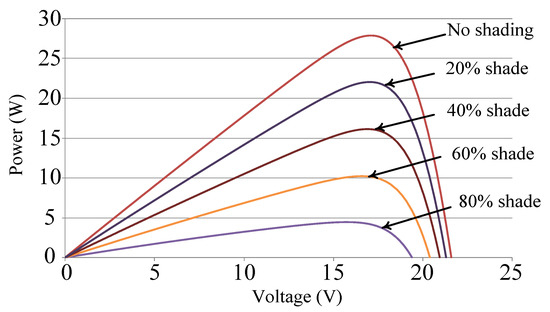
Figure 1. Power–voltage (P–V) characteristic curve of a single photovoltaic module with diverse percentages of shade.

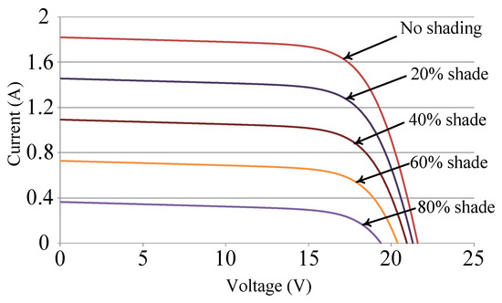
Figure 2. Current–voltage (I–V) characteristic curve of a single photovoltaic module with diverse percentages of shade.

Figure 3 illustrates the P–V and I–V characteristic curves of a photovoltaic module array with a four series and one parallel structure and one module under 30% shade. Because the photovoltaic module array is made up of four photovoltaic modules in series, one of which is shaded by 30%, and the rest is not shaded. Consequently, there are two kinds of irradiation conditions, it will appear two peaks in the P–V characteristic curve of a PV module array. The rest of the situation, and so on. Therefore, a multi-peak phenomenon and a considerable decrease in the maximum power output can be observed in the P–V characteristic curve. Figure 4 illustrates the P–V and I–V characteristic curves of a photovoltaic module array with a four series and one parallel structure and one module that malfunctioned. Due to the malfunction of the module in question, no output current was observed. Moreover, the current outputs of the normal modules flowed to the load through the bypass diode of the malfunctioning module. Thus, a normal operation of the photovoltaic module array could be maintained; however, the total power output of the array was equal to the power output of only three modules.

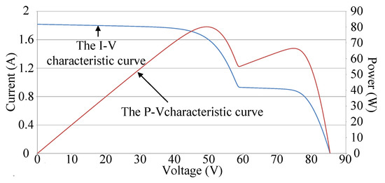
Figure 3. P–V and I–V characteristic curves of the photovoltaic module array with a four series and one parallel structure and one module under 30% shade.

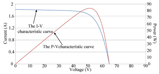
Figure 4. P–V and I–V characteristic curves of the photovoltaic module array with a four series and one parallel structure and one malfunctioning module.

3. TLBO Algorithm

The TLBO algorithm is a swarm intelligence optimization algorithm proposed by Rao, Savsani, and Vakharia in 2011 [17]. This algorithm is inspired by the learning pattern between teachers and learners. It involves dividing a group into a teacher and several learners. The learners learn from the teacher and other learners to improve their overall performance.

3.1. Conventional TLBO Algorithm

The TLBO algorithm [14] has been applied to MPPT in photovoltaic module arrays. The parameters used in the conventional TLBO algorithm are defined as follows:

Number of learners (N_p): the total number of learners in a class.

Number of iterations (E): the number of times learners learn and are taught.

Target performance (X_j,k): the performance of learner k in subject j; five subjects were considered in this study.

Mean performance (M): the mean performance of the entire class.

Teaching step (r_i): the parameters that enhance the diversification of the learner’s difference mean; in this study, the teaching stride had a random value between 0 and 1.

Teaching factor (T_F): the parameter value of the teacher’s teaching of the learners; in this study, the teaching factor in a randomly generated value of 1 or 2.

The steps in the conventional TLBO algorithm are as follows:

Step 1:

Set the number of learners (N_P), number of subjects (m), and the number of iterations (E).

Step 2:

Initialize the class and define the parameters as follows:

(1)

Random learner: $X_k\subset \{X_1,X_2,\dots X_{N_P}\}$

(2)

Random subject: $X_j\subset \{X_1,X_2,\dots X_m\}$

(3)

Performance of learner k in subject j: G_j,k

Step 3:

In the teacher phase, set the teaching step (r_i), teaching factor (T_F), and performance of the best learner (X_{j,k_best}). Calculate the mean result of the class following Equation (1); calculate the learners’ difference mean by applying Equation (2); and renew all the learners’ target performance in the learner phase by following Equation (3).

$$M={\displaystyle \sum _{k=1}^{N_P}\frac{X_k}{N_P}},$$

(1)

$$Different\_Mea{n}_{j,k}=r_i(X_{j,k\_best}-T_F\cdot M),$$

(2)

$$X_{j,k(new)}=X_{j,k(old)}+Different\_Mea{n}_{j,k}.$$

(3)

Step 4:

In the learning process, assume that a randomly selected learner X_H and learner X_I learn from each other. When the performance of X_H is superior to that for X_I, apply Equation (4). If the performance of X_I is superior to that for X_H, apply Equation (5).

$$X^{\prime }{}_{j,k(new)}=X_{j,k(old)}+r_i(X_{j,H}-X_{j,I}),$$

(4)

$$X^{\prime }{}_{j,k(new)}=X_{j,k(old)}+r_i(X_{j,I}-X_{j,H}),$$

(5)

$$X_H,X_I\subset \{X_1,X_2,\cdots X_{N_P}\}$$

Step 5:

Repeat Steps 4 and 5 until the criterion for terminating the iteration is met.

In the teaching phase of the conventional TLBO algorithm, the teaching factor (T_F) is randomly selected as 1 or 2, which is not completely suitable for all learners. Because the ability of each learner varies, applying inappropriate teaching factors results in the teacher using wrong methods for teaching. Thus, the learners cannot successfully absorb the learning experience, and their learning efficiency decreases. In the learner phase, each learner learns from another randomly selected learner, which may worsen the learning effect. To avoid such problems, an improved TLBO algorithm was proposed [14]. In this study, an improved TLBO algorithm with superior tracking efficiency is proposed on the basis of the TLBO algorithm proposed in Reference [14].

3.2. Proposed Improved TLBO Algorithm

The improvements in the proposed TLBO algorithm are as follows:

• Teaching factors are automatically adjusted according to the absorption ability of all the learners in the class. The adjustment measure is presented in Equation (6). The automatic adjustment in the teaching factor allows the teacher to assess the learning level of the entire class and design learning methods that increase the overall performance of the class. In contrast to the TLBO algorithm proposed in Reference [14], the proposed algorithm focuses on the entire class rather than on individual learners.

  $$T_F=\frac{M}{X_{j,k\_best}}.$$

  (6)
• Rather than two randomly selected learners learning from each other, all the learners in the class learn from the learner with the best result in the learner phase.
• In the learner phase, a self-learning function is added so that each learner can adjust according to past experience, as presented in Equation (7).

  $$X^{″}{}_{j,k(new)}=X^{\prime }{}_{j,k(new)}+r_i(X^{\prime }{}_{j,k(new)}-X^{\prime }{}_{j,k-1(new)}).$$

  (7)

In Equation (2), if X_{j,k_best} remains the same when M and T_F increase, Different_Mean_j,k decreases. Similarly, when MPPT is being performed for a photovoltaic module array, the shorter the distance from the maximum power point, the smaller the tracking step will become. By contrast, the longer the distance with the maximum power point is, the larger the tracking step becomes. The MPPT procedures of the proposed improved TLBO algorithm are illustrated in Figure 5.

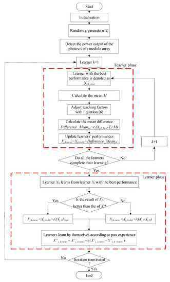
Figure 5. Flowchart of maximum power point tracking (MPPT) based on the proposed improved teacher-learning-based optimization (TLBO).

3.3. Maximum Power Tracker of the Proposed Improved TLBO Algorithm

Figure 6 illustrates the structure of the proposed maximum power tracker based on the improved TLBO algorithm for photovoltaic module arrays. It mainly comprises two parts: a DC/DC boost converter and the maximum power point tracker and controller based on the proposed improved TLBO algorithm. The controller controlled the on–off duty cycle of the boost converter so that the photovoltaic module array still yielded maximum power output, even when some of its modules malfunctioned or were under shade.

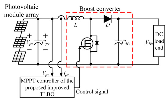
Figure 6. Structure of the maximum power point tracker based on the proposed improved TLBO algorithm.

Table 2 lists the design parameters of the elements of the DC/DC boost converter circuit used in this study [18], and Table 3 presents the set parameters of the conventional TLBO algorithm. For the proposed improved TLBO algorithm, the T_F value in Table 3 was replaced with the set parameter value in Table 4, and the other parameters remained identical. The algorithm was tested on a photovoltaic module array in five working conditions, which are listed in Table 5.

Table 2. Specifications of the main elements of a boost converter.

Item	Specifications
Storage induction (L)	1.5 mH, withstand current of 10A
Filter capacity (Cin)	470 uF, withstand voltage of 450 V
Filter capacity (Cout)	470 uF, withstand voltage of 450 V
Fast diode (D) IQBD30E60A1	Withstand voltage VRRM = 600 V, withstand current IFAV = 30 A
Power semiconductor IXGH48N60C3D1	Withstand voltage VDSS = 600 V, withstand current ID = 30 A

Table 3. Set parameter values of the conventional TLBO algorithm.

Parameter Name	Set Parameter Values
Number of learners (NP)	4
Number of iterations (E)	40
Teaching step (ri)	Randomly selected between 0 and 1
Teaching factor (TF)	1 or 2

Table 4. Set parameter values of the proposed improved TLBO algorithm.

Parameter Name	Set Parameter Values
Teaching factor (TF)	$T_F=\frac{M}{X_{j,k\_best}}$

Table 5. Connection patterns and shade conditions in the five selected test cases.

Case	Connection Patterns and Shade Conditions	Number of Peak(s) in the P–V Curve
1	One series and one parallel: 0% shade	1
2	Two series and one parallel: 0% shade + 40% shade	2
3	Three series and one parallel: 0% shade + 30% shade + 70% shade	3
4	Three series and one parallel: 0% shade + 30% shade + 50% shade + 70% shade	4
5	Three series and two parallels: (30% shade + 0% shade)/(0% shade + 50% shade)	2

Note: “+” signifies “series” and “//” signifies “parallel”.

4. Simulation Results

Solar Pro, a photovoltaic system simulation software program, was used to perform simulation modeling of a SANYO HIP 2717 photovoltaic module. Simulation was performed for photovoltaic module arrays according to the connection patterns and shading ratios specified in Table 5. Statistics of the characteristic curves of the arrays were collected and input into MATLAB software to simulate the P–V characteristic curves of the photovoltaic module arrays under different connection patterns and shading ratios and to compare the MPPT results when applying diverse TLBO algorithms.

4.1. Case 1: One Series and One Parallel (No Shading)

Figure 7 illustrates the P–V characteristic curve of a HIP-2717 photovoltaic module without shading. This curve indicates that when the photovoltaic module array was in a normal state without shading, its maximum power output was approximately 27.8 W. Figure 8 displays the simulation results when applying diverse TLBO algorithms to perform MPPT. The results indicate that all the three MPPT techniques could obtain the maximum power point. Moreover, the proposed improved TLBO algorithm had a faster tracking time than the conventional TLBO algorithm and the existing improved TLBO algorithm proposed in Reference [14].

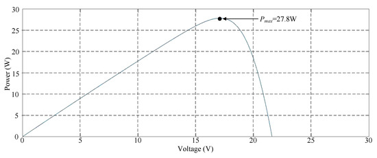
Figure 7. Simulated power–voltage (P–V) characteristic curve for Case 1.

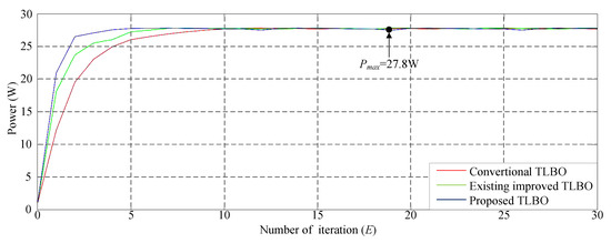
Figure 8. Simulation results of MPPT performed using diverse TLBO algorithms in Case 1.

4.2. Case 2: Two Series and One Parallel (0% Shade + 40% Shade)

Figure 9 illustrates the photovoltaic module array with a two series and one parallel structure. The P–V characteristic curve of the photovoltaic module under 40% shade exhibited a twin-peak phenomenon. The real maximum power point (35.5 W) was at the peak to the right. Figure 10 depicts the simulation results of MPPT performed with different TLBO algorithms. Figure 10 indicates that the three algorithms that could obtain the real maximum power point had considerably different numbers of iterations. The method proposed in this study could obtain the real maximum power point faster than the other two methods could.

Figure 9. Simulated P–V characteristic curve for Case 2.

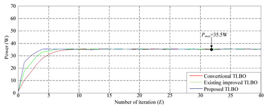
Figure 10. Simulation results of MPPT performed using the three TLBO algorithms in Case 2.

4.3. Case 3: Three Series and One Parallel (0% Shade + 30% Shade + 70% Shade)

Figure 11 depicts the simulated P–V characteristic curve for Case 3. In the photovoltaic module array, one module was under 30% shade and one was under 70% shade, which resulted in the triple-peak phenomenon of the characteristic curve. The real maximum power point (37.92 W) was at the middle peak. Figure 12 displays the simulation results of MPPT when applying the conventional TLBO algorithm, TLBO algorithm proposed in Reference [14], and TLBO algorithm proposed in this study. As displayed in Figure 12, the conventional TLBO algorithm required the highest time to obtain the real maximum power point (37.9 W). The tracking speed of the TLBO algorithm proposed in Reference [14] was faster than that of the conventional TLBO algorithm; however, its precision and speed in obtaining the maximum power point (37.9 W) were inferior to those of the TLBO algorithm proposed in this study.

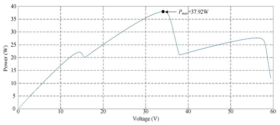
Figure 11. Simulated P–V characteristic curve for Case 3.

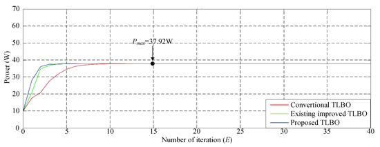
Figure 12. Simulation results of MPPT performed using the three TLBO algorithms in Case 3.

4.4. Case 4: Three Series and One Parallel (0% Shade + 30% Shade + 50% Shade + 70% Shade)

Figure 13 depicts the simulated P–V characteristic curves for Case 4. Due to the increased number of series in the photovoltaic module array, one module each was under 30%, 50%, and 70% shade. Consequently, a four-peak phenomenon was observed in the P–V characteristic curve, and the real maximum power point (43.5 W) was at the third peak. Figure 14 displays the simulation results when conducting MPPT by using the conventional TLBO algorithm, TLBO algorithm proposed in Reference [14], and the TLBO algorithm proposed in this study. As illustrated in Figure 14, the tracking speed of the TLBO algorithm proposed in this study considerably exceeded that of the conventional TLBO algorithm and TLBO algorithm proposed in Reference [14].

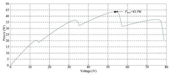
Figure 13. Simulated P–V characteristic curve for Case 4.

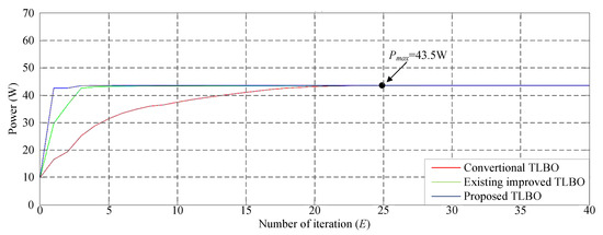
Figure 14. Simulation results of MPPT performed using the three TLBO algorithms in Case 4.

4.5. Case 5: Three Series and Two Parallels (30% Shade +0% Shade)/(0% Shade + 50% Shade)

Figure 15 illustrates the simulated P–V characteristic curve for Case 5. In the photovoltaic module array, one module was under 30% shade and one module was under 50% shade. Consequently, a double-peak phenomenon was observed in the P–V characteristic curve, with the real maximum power point (66.7 W) occurring at the peak to the right. Figure 16 displays the simulation results of MPPT when applying the conventional TLBO algorithm, TLBO algorithm proposed in Reference [14], and TLBO algorithm proposed in this study. The figure indicates that the conventional TLBO algorithm required more iterations than the TLBO algorithms proposed in Reference [10] and this study to obtain the real maximum power point. In addition, the TLBO algorithm proposed in this study had a considerably higher tracking efficiency than the TLBO algorithm proposed in Reference [14].

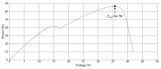
Figure 15. Simulated P–V characteristic curve for Case 5.

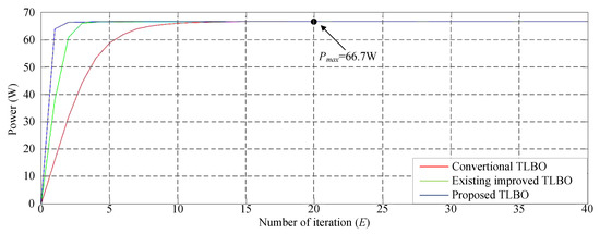
Figure 16. Simulation results of MPPT performed using the three TLBO algorithms in Case 5.

5. Practical Test Results

The P–V and I–V characteristic curves of PV module arrays under different shading ratios were measured using an MP 170 I–V checker manufactured by EKO Instruments CO. Ltd. (Tokyo, Japan) [19]. The aim is to tell whether the global MPPs in the 5 testing cases listed in Table 5 can be tracked as expected using TBLO MPPT proposed in this study. Figure 17 shows the photograph of the experimental setup. To analyze precisely the tracking of the four MPPT algorithms when the P–V characteristic curves exhibited multi-peak phenomena, the MP-170 measuring instrument was used for measuring the P–V characteristic curves of a HIP 2717 photovoltaic module simulator [20] in five cases. Moreover, the four methods were used to perform practical tests on MPPT. The five shade conditions are specified in Table 5.

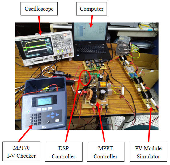
Figure 17. The photograph of the experimental setup.

5.1. Case 1: One Series and One Parallel (No Shading)

Figure 18 illustrates the practical P–V characteristic curve for Case 1 when conducting the MP-170 practical test. When the photovoltaic module array was in a normal state without shading, its maximum power output was approximately 27.8W. Figure 19, Figure 20 and Figure 21 display the practical test results of MPPT in Case 1 when applying the conventional TLBO algorithm, TLBO algorithm proposed in Reference [14], and TLBO algorithm proposed in this study, respectively. The figures indicate that the three TLBO algorithms had similar tracking efficiencies. However, the TLBO algorithm proposed in this study outperformed the other two algorithms in terms of the tracking speed and stability.

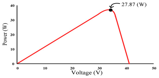
Figure 18. Practical P–V characteristic curve for Case 1.

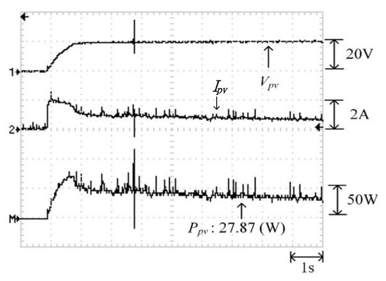
Figure 19. Practical test results of MPPT in Case 1 when applying the conventional TLBO algorithm.

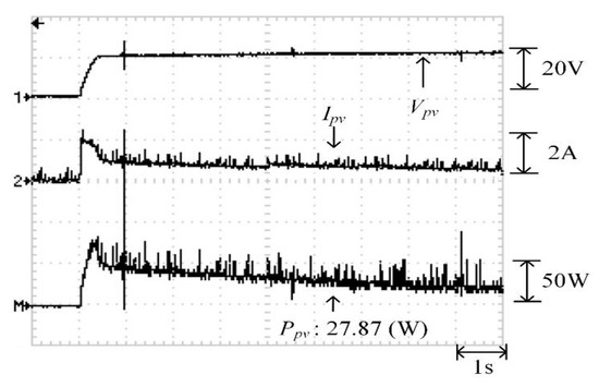
Figure 20. Practical test results of MPPT in Case 1 when applying the TLBO algorithm proposed in Reference [14].

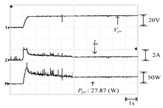
Figure 21. Practical test results of MPPT in Case 1 when applying the TLBO algorithm proposed in this study.

5.2. Case 2: Two Series and One Parallel (0% Shade + 40% Shade)

Figure 22 depicts the practical P–V characteristic curve for Case 2 when performing the MP-170 practical test under a double-peak phenomenon. The real maximum power point (35.94 W) was at the peak to the right. Moreover, Figure 23, Figure 24 and Figure 25 illustrate the practical test results of MPPT in Case 2 when applying the conventional TLBO, TLBO algorithm proposed in Reference [14], and TLBO algorithm proposed in this study. The figures indicate that the lowest speed of escaping from a local optimum was achieved with the conventional TLBO algorithm, which exhibited a tracking time of 1 s. The tracking time for the TLBO algorithm proposed in Reference [14] was 0.6 s. The highest speed of escaping from a local optimum was observed for the TLBO algorithm proposed in this study. This algorithm also successfully obtained the real maximum power point (35.94 W) with 0.3 s of tracking.

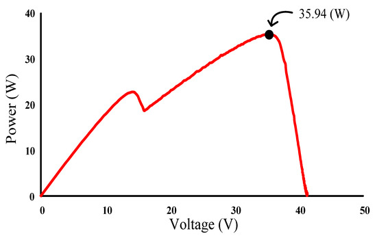
Figure 22. Practical P–V characteristic curve for Case 2.

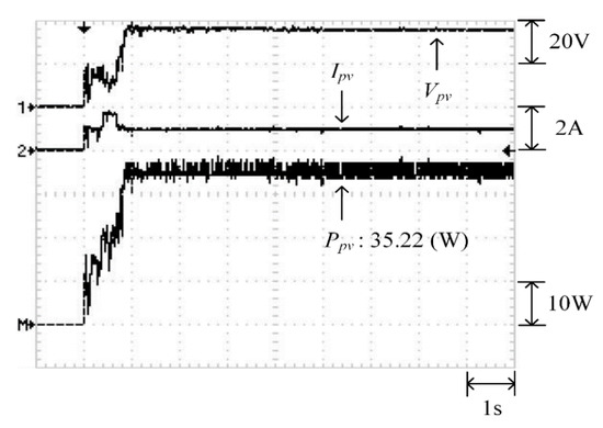
Figure 23. Practical test results of MPPT in Case 2 when applying the conventional TLBO algorithm.

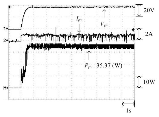
Figure 24. Practical test results of MPPT in Case 2 when applying the TLBO algorithm proposed in Reference [14].

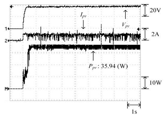
Figure 25. Practical test results of MPPT in Case 2 when applying the TLBO algorithm proposed in this study.

5.3. Case 3: Three Series and One Parallel (0% Shade + 30% Shade + 70% Shade)

Figure 26 displays the P–V characteristic curve for Case 3, in which a three-peak phenomenon was observed and the real maximum power point (37.92 W) was at the middle peak. Moreover, Figure 27, Figure 28 and Figure 29 depict the practical test results of MPPT in Case 3 when applying the conventional TLBO algorithm, TLBO algorithm proposed in Reference [14], and TLBO algorithm proposed in this study, respectively. The figures indicate the risk of falling easily into a local optimum when applying the conventional TLBO algorithm, which required 4 s to obtain the real maximum power point. The tracking speed of the TLBO algorithm proposed in Reference [14] (tracking time: 1.1 s) was higher than that of the conventional TLBO algorithm but lower than that of the TLBO algorithm proposed in this study, which only required 0.45 s to obtain the real maximum power point (37.92 W). Thus, the proposed algorithm exhibited improvements over the other two algorithms in terms of precision and efficiency of MPPT.

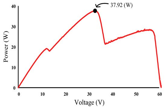
Figure 26. Practical P–V characteristic curve for Case 3.

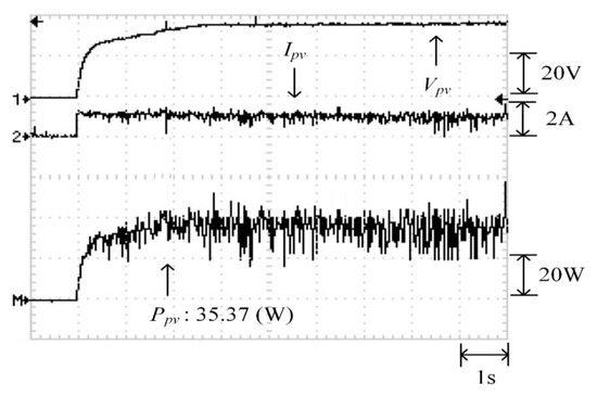
Figure 27. Practical test results of MPPT in Case 3 when applying the existing TLBO algorithm.

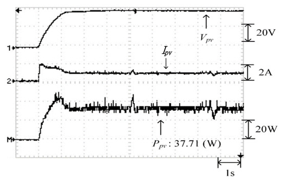
Figure 28. Practical test results of MPPT in Case 3 when applying the TLBO algorithm proposed in Reference [14].

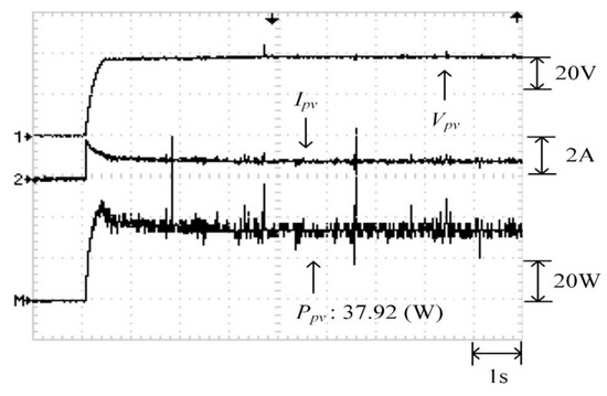
Figure 29. Practical test results of MPPT in Case 3 when applying the TLBO algorithm proposed in this study.

5.4. Case 4: Four Series and One Parallel (0% Shade + 30% Shade + 50% Shade + 70% Shade)

Figure 30 depicts the practical P–V characteristic curve for Case 4, which exhibits a four-peak phenomenon. The real maximum power point (43.55 W) was at the middle peak. Figure 31, Figure 32 and Figure 33 illustrate the practical test results of MPPT in Case 4 when applying the conventional TLBO algorithm, TLBO algorithm proposed in Reference [14], and TLBO algorithm proposed in this study, respectively. The figures indicate the impossibility of successfully escaping a local optimum within a certain number of iterations when applying the conventional TLBO algorithm. Consequently, the time for tracking reached 7 s and the maximum power output obtained was only 35.62 W with the conventional TLBO algorithm. The TLBO algorithm proposed in Reference [14] required 4 s to escape from a local optimum when obtaining the maximum power point. The maximum power point obtained with the TLBO algorithm propose in Reference [10] under the steady state was 42.59 W, which still differed from the real maximum power point (43.55 W). The TLBO algorithm proposed in this study had a lower tracking time than the other two algorithms. The time required for obtaining the real maximum power point (43.55 W) was only 1.8 s, which verified the superiority of the proposed algorithm in terms of the tracking precision and speed.

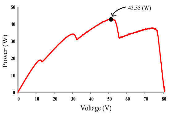
Figure 30. Practical P–V characteristic curve for Case 4.

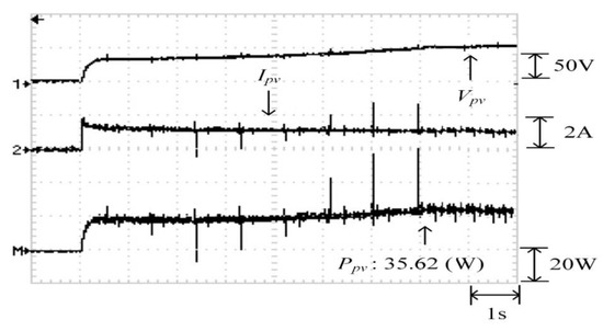
Figure 31. Practical test results of MPPT in Case 4 when applying the conventional TLBO algorithm.

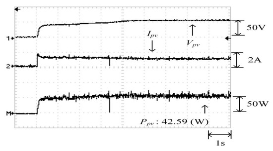
Figure 32. Practical test results of MPPT in Case 4 when applying the TLBO algorithm proposed in Reference [14].

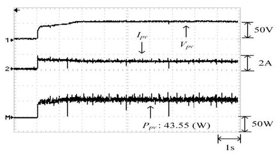
Figure 33. Practical test results of MPPT in Case 4 when applying the TLBO algorithm proposed in this study.

5.5. Case 5: Two Series and Two Parallels (30% Shade + 0% Shade)/(50% Shade + 0% Shade)

Figure 34 illustrates the practical P–V characteristic curve for Case 5, which exhibits a double-peak phenomenon. The real maximum power point (66.74 W) was located at the peak to the right. Figure 35, Figure 36 and Figure 37 depict the practical tests results of MPPT in Case 5 when applying the conventional TLBO algorithm, TLBO algorithm proposed in Reference [14] and TLBO algorithm proposed in this study, respectively. The figures indicate that the conventional TLBO algorithm required the longest time to escape a local optimum. Consequently, the tracking time of the TLBO algorithm was 1.6 s, which was longer than the tracking time of the other two TLBO algorithms. The tracking time required by the TLBO algorithm proposed in this study was only 0.3 s. The tracking time of the proposed TLBO algorithm was lower than that of the TLBO algorithm proposed in Reference [14] (1.1 s).

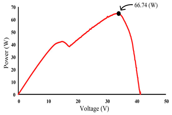
Figure 34. Practical P–V characteristic curve for Case 5.

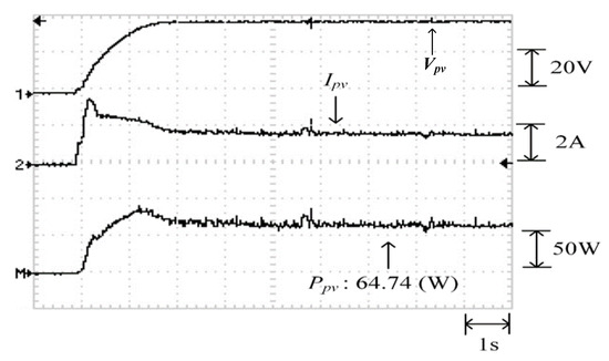
Figure 35. Practical test results of MPPT in Case 5 when applying the conventional TLBO algorithm.

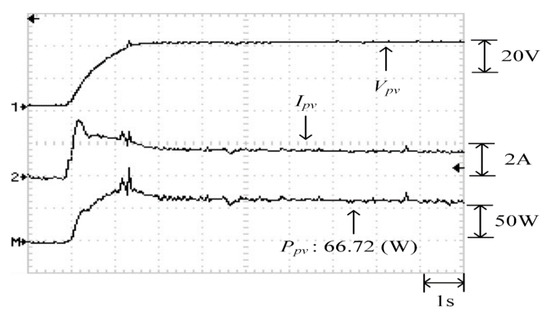
Figure 36. Practical test results of MPPT in Case 5 when applying the TLBO algorithm proposed in Reference [14].

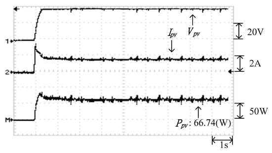
Figure 37. Practical test results of MPPT in Case 5 when applying the proposed TLBO algorithm.

Table 6 gives the performance comparison in terms of the average tracking time and the average maximum power for 10 trials among the proposed improved TBLO algorithm, TLBO algorithm proposed in Reference [14], conventional TLBO algorithm, and using the 0.8V_oc model proposed in Reference [4].

Table 6. Comparison of the practical tests results for the five selected cases.

Case	Number of Peak(s) of the P–V Curve	Model Proposed in Reference [4]		Conventional TLBO		TLBO Proposed in Reference [14]		TLBO Proposed in This Study
		Average Tracking Time	Average Maximum Power	Average Tracking Time	Average Maximum Power	Average Tracking Time	Average Maximum Power	Average Tracking Time	Average Maximum Power
1	1	0.9 s	27.87 W	0.8 s	27.87 W	0.4 s	27.87 W	0.2 s	27.87 W
2	2	1.2 s	35.25 W	1.0 s	35.22 W	0.6 s	35.37 W	0.3 s	35.94 W
3	3	1.91 s	35.47 W	1.89 s	35.37 W	1.1 s	37.71 W	0.45 s	37.92 W
4	4	Tracking failed	35.71 W	Tracking failed	35.73 W	3.5 s	42.59 W	1.2 s	43.55 W
5	2	1.31 s	64.58 W	1.22 s	64.68 W	0.67 s	66.74 W	0.4 s	66.74 W

6. Conclusions

An intelligent maximum power point tracker was developed in this study for photovoltaic module arrays. MPPT techniques were improved on the basis of the conventional TLBO algorithm and existing improved TLBO algorithm so that the teaching factors of the TLBO algorithm could be automatically adjusted according to the learning efficiency of the learners in a class and all the learners could learn from the best individual in the class. Moreover, each learner would be able to learn according to their past experience, thus improving the learning efficiency. In this manner, when some shaded or malfunctioning modules of the photovoltaic module array led to the multi-peak phenomenon in the P–V characteristic curve, the problem regarding the impossibility of obtaining the real maximum power point in conventional MPPT could be avoided. Consequently, the maximum power point tracker continued functioning at the maximum power point despite the variations in the sunshine and shade conditions. The simulation results proved that in the case of photovoltaic module arrays with diverse connection patterns and percentages of shading, the tracking speed of MPPT was faster with the proposed TLBO algorithm than with the conventional TLBO algorithm and existing improved TLBO algorithm. In addition, some experimental results under different connected configuration and shading conditions show that the MPPT tracking speed of the proposed improved TLBO algorithm is 2–4 times faster than those of the existed improved TLBO algorithm and conventional TLBO algorithm. Therefore, the power generating efficiency of the proposed method is improved by about 2–3% compared with the existed improved TLBO algorithm and conventional TLBO algorithm.

References

- Femia, N.; Granozio, D.; Petrone, G.; Spagnuolo, G.; Vitelli, M. Predictive and adaptive MPPT perturb and observe method. IEEE Trans. Aerosp. Electron. Syst. 2007, 43, 934–950. [Google Scholar] [CrossRef]
- Esram, T.T.; Chapman, P.L. Comparison of photovoltaic array maximum power point tracking techniques. IEEE Trans. Energy Convers. 2007, 22, 439–449. [Google Scholar] [CrossRef]
- Chao, L.; Sang, P.P.; Vijay, R.; Kaushik, R. Low-overhead maximum power point tracking for micro-scale solar energy harvesting systems. In Proceedings of the 25th International conference on VLSI design, Hyderabad, India, 25 August 2011; pp. 215–220. [Google Scholar]
- Bi, Z.; Ma, J.; Man, K.L.; Smith, J.S.; Yue, Y.; Wen, H. Global MPPT method for photovoltaic systems operating under partial shading conditions using the 0.8VOC model. In Proceedings of the 2019 IEEE International Conference on Environment and Electrical Engineering and 2019 IEEE Industrial and Commercial Power Systems Europe (EEEIC/I&CPS Europe), Genova, Italy, 11–14 June 2019; pp. 1–6. [Google Scholar]
- Elif, S.M.; Chao, L.; Vijay, R.; Kaushik, R. Modeling, design and cross-layer optimization of polysilicon solar cell based micro-scale energy harvesting systems. In Proceedings of the 2012 ACM/IEEE International Symposium on Low Power Electronics and Design, Redondo Beach, CA, USA, 30 July–1 August 2012; pp. 123–128. [Google Scholar]
- Rehan, A.; Bernhard, B.; Stefan, D.; Lukas, S.; Pratyush, K. Optimal power management with guaranteed minimum energy utilization for solar energy harvesting systems. ACM Trans. Embed. Comput. Syst. 2019, 18, 1–26. [Google Scholar]
- Patel, H.; Agarwal, V. MATLAB-based modeling to study the effectsof partial shading on PV array characteristics. IEEE Trans. Energy Convers. 2008, 23, 302–310. [Google Scholar] [CrossRef]
- Mirjalili, S.S.M.; Lewis, A. Grey wolf optimizer. Engine Softw. 2014, 69, 46–61. [Google Scholar] [CrossRef]
- Dorigo, M.; Birattari, M.; Stutzle, T. Ant colony optimization. IEEE Comput. Intell. Mag. 2006, 1, 28–39. [Google Scholar] [CrossRef]
- Gao, W.; Liu, S.; Huang, L. A global best artificial bee colony algorithm for global optimization. J. Comput. Appl. Math. 2012, 236, 2741–2753. [Google Scholar] [CrossRef]
- Pragallapati, N.; Sen, T.; Agarwal, V. Adaptive velocity PSO for global maximum power control of a PV array under nonuniform irradiation conditions. IEEE J. Photovolt. 2017, 7, 624–639. [Google Scholar] [CrossRef]
- Sen, T.; Pragallapati, N.; Agarwal, V.; Kumar, R. Global maximum power point tracking of PV arrays under partial shading conditions using a modified particle velocity-based PSO technique. IET Renew. Power Gener. 2018, 12, 555–564. [Google Scholar] [CrossRef]
- Rao, R.V.; Savsani, V.J.; Vakharia, D.P. Teaching-learning-based optimization: A novel method for constrained mechanical design optimization problems. Comput. Aided Des. 2011, 43, 303–315. [Google Scholar] [CrossRef]
- Chao, K.H.; Wu, M.C. Global maximum power point tracking (MPPT) of a photovoltaic module array constructed through improved teaching-learning-based optimization. Energies 2016, 9, 986. [Google Scholar] [CrossRef]
- SANYO HIP 2717 Datasheet. Available online: http://iris.nyit.edu/~mbertome/solardecathlon/SDClerical/SD_DESIGN+DEVELOPMENT/091804_Sanyo190HITBrochure.pdf (accessed on 18 December 2019).
- Solar Pro Website. Available online: http://www.lapsys.co.jp/english/e_products/e_pamphlet/sp_e.pdf (accessed on 18 December 2019).
- Rao, R.V.; Patel, V. An elitist teaching-learning-based optimization algorithm for solving complex constrained optimization problems. Int. J. Ind. Eng. Comput. 2012, 3, 535–560. [Google Scholar] [CrossRef]
- Hart, D.W. Introduction to Power Electronics; Prentice Hall: New York, NY, USA, 2003. [Google Scholar]
- MP-170 Brochure. Available online: http://www.environmental-expert.com/products/model-mp-170-iv-checker-80092 (accessed on 21 August 2020).
- Chao, K.H.; Chao, Y.W.; Chen, J.P. A circuit-based photovoltaic module simulator with shadow and fault setting. Int. J. Electron. 2016, 103, 424–438. [Google Scholar] [CrossRef]
© 2020 by the authors. Licensee MDPI, Basel, Switzerland. This article is an open access article distributed under the terms and conditions of the Creative Commons Attribution (CC BY) license (http://creativecommons.org/licenses/by/4.0/).