Abstract
Spontaneous water imbibition plays an imperative role in the development of shale or tight oil reservoirs. Spontaneous water imbibition is helpful in the extraction of crude oil from the matrix, although it decreases the relative permeability of the hydrocarbon phase dramatically. The dynamic pore-scale network modeling of water imbibition in shale and tight reservoirs is presented in this work; pore network generation, local capillary pressure function, conductance calculation and boundary conditions for imbibition are all presented in detail in this paper. The pore network is generated based on the characteristics of Barnett shale formations, and the corresponding laboratory imbibition experiments are matched using this established dynamic pore network model. The effects of the wettability, throat aspect ratio, viscosity, shape factor, micro-fractures, etc. are all investigated in this work. Attempts are made to investigate the water imbibition mechanisms from a micro-scale perspective. According to the simulated results, wettability dominates the imbibition characteristics. Besides this, the viscous effects including viscosity, initial capillary pressure and micro-fractures increase the imbibition rate, while the final recovery factor is more controlled by the capillarity effect including the cross-area shape factor, contact angle and the average pore-throat aspect ratio.
1. Introduction
The spontaneous water imbibition phenomenon is commonly encountered in the development of shale or tight reservoirs. Water imbibition is helpful for the replacement of oil from the matrix and increases the oil recovery, while it decreases the relative permeability of the hydrocarbon phase dramatically, which is detrimental to the production rate and recovery factor [1,2]. Generally, the capillarity is believed to be the controlling factor for the imbibition of water in shale and tight formations. Analogous to waterflooded carbonate reservoirs [3,4,5], taking full advantage of water imbibition to yield the highest oil recovery is a major concern for the development of shale and tight reservoirs. Moreover, surfactant additives are proposed to alter the formation wettability and improve the performance of water imbibition [6,7,8]. Large numbers of experimental studies of spontaneous imbibition have been reported in the literature for both conventional [9,10,11,12,13] and unconventional reservoirs [14,15,16]. Large numbers of analytical models based on a bundle of capillary tubes have been proposed following the early works by Lucas [17]. Viscosity ratios, the tortuosity of capillary tubes, the shapes of cross-sectional areas and the assumption of fractal porous media are involved in these models [18,19]. An attempt has been made to find a universal upscaling equation since the imbibition rate and its recovery factor is sensitive to the sample size; i.e., the characteristic length. Unfortunately, these upscaling techniques are still not applicable for some other factors including wettability, complex rock structures and a wide range of fluid viscosities, etc.
Recently, scholars have become more focused on the micro-scale studies of water imbibition [20], and pore-scale network models have therefore been proposed to simulate this process. There are two types of pore-scale network fluid flow simulation models: quasi-static and dynamic models. For quasi-static models, the fluid flow is controlled by capillarity effects and the viscous forces are neglected. In contrast, inspired by the continuum reservoir simulation method, the dynamic pore network models consider both capillarity and viscous effects. For every increase or decrease of capillary pressures, the two-phase displacement mechanisms—including the piston-like entry of the non-wetting phase, the piston-like throat filling of the wetting phase, the snap-off of the non-wetting phase and the cooperative pore filling of the wetting phase [21,22]—are considered by quasi-static models. Based on the calculated capillary pressure and relative permeability from quasi-static models, the spontaneous imbibition process can then be simulated using conventional reservoir simulators or some simple analytical solutions [23,24,25,26]. However, we cannot simulate the process of imbibition directly from the quasi-static model, as not all calculated macro-properties have a relationship with time. Meanwhile, the quasi-static models assume capillary-dominated flow, and the capillary number is assumed to be less than 10−5 [27,28].
For the dynamic pore network models, Sheng and Thompson [29] reviewed and divided the dynamic models into three categories: semi-dynamic models (perturbative models), Washburn equation-based dynamic models and coupled dynamic models. The semi-dynamic models separately calculate each phase pressure and update the saturation profiles by ranking the pore elements using a defined global potential which is a combination of the local capillary pressure, viscous pressure drop and gravity. This idea was first derived by Blunt and Scher [30] and then further developed by Hughes and Blunt [31], Idowu and Blunt [32] and Aghaei and Piri [33]. The second type of dynamic model uses the Washburn equation to combine the viscous and capillary forces. Aker et al. [34] did pioneering work and established a framework in this area. Accounting for the wetting film flow, this model is further improved [35,36]. The third type of dynamic model is based on the mass conservation of multiphase flow in every pore element, which is similar to the conventional macroscale reservoir simulation. The Implicit Pressure and Explicit Saturation (IMPES) algorithm is applied to solve the dynamic model. As noted by Khayrat [37], there are two key difficulties resulting in the instability of numerical solutions: (1) local rules in dynamic network models cause a strong non-linearity in the non-wetting conductance because of the occurrence of non-continuity; (2) the capillary pressure is fully coupled within the displacement process, which is a sensitive function of phase saturation. Therefore, an appropriate algorithm is needed to ensure numerical stability, and several related studies have been conducted [38,39].
In this work, we propose a dynamic pore-scale network fluid flow simulation model that simulates the process of spontaneous water imbibition in shale or tight formations. The newly derived mathematical model and corresponding solution algorithm are presented. The proposed model is first applied and validated for Barnett shale formations for the single-phase flow, and then the spontaneous imbibition process is simulated and corresponding systematical sensitivity studies are conducted. Attempts are made to propose an approach to investigate the spontaneous water imbibition mechanisms from a micro-scale perspective.
2. Dynamic Pore Network Modelling of Water Imbibition
2.1. Pore Network Generation
Capillary tube models are suitable for single-phase flow; however, they fail to simulate the multiphase flow scenarios in a porous medium. Pore-scale network models bridge the gap between the single capillary tube model and the porous media system. Firstly, we need to generate the pore network for the studied porous media before simulating two-phase flow processes within them. A structured network consisting of nodes and connecting bonds is used, where nodes are assigned as pore bodies and bonds as pore-throats. A truncated lognormal density distribution function (c.f. Equation (1)) commonly yields a good fit for the profiles of the pore-throat distribution of reservoir rocks [38]. Since the larger pores tend to be connected with larger throats, we cannot randomly assign the pore bodies connected to the pore-throats; here, we sort the pore bodies by the mean values of the connected throats’ radii, and then the corresponding sorted pore body radii are assigned.
where, r refers to the radius of pores or throats, and refer to the mean, maximum and minimum radii of pores or throats, respectively; is the standard derivation of the radius distribution.
Following the work by Mason and Morrow [40], in which they studied the capillarity behavior of drainage and imbibition in irregular perfect wetting triangular micro-tubes, the definition of the shape factor is used as shown in Equation (2).
where and are the cross-sectional area and the perimeter of a pore or throat.
For a cross-sectional shape, if we define the corner half angles of the triangle as , two constraints need to be met, given a shape factor value:
where is randomly chosen to range from the lower and upper boundaries in Equations (5) and (6).
The mean values of Equations (5) and (6) are used; thus, the smallest half corner angle can be calculated by
Finally, is calculated by applying Equation (3). In this way, we can use a single shape factor for the whole pore network. Therefore, one single shape factor will help us to use a single dimensionless local capillary function for every pore or throat with variable wetting phase saturation, which will be presented later. The schematic of the pore network and the triangular cross-section of every pore element are presented in Figure 1.
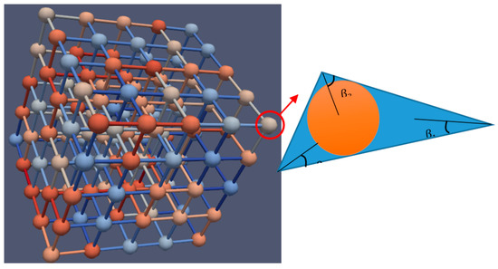
Figure 1.
Schematic of the pore network and the triangular cross-section of every pore element.
2.2. Control Equations and Conductance Calculation
The proposed dynamic pore-scale network model is based on the following assumptions:
(1) The volume of throats is negligible compared with that of pore bodies, while the throats control the conductances between pore bodies; (2) the pressure field is continuous, and an upwind scheme is used for the numerical treatment, while the saturation could be discontinuous, especially for the connecting throats; (3) fluids are assumed to be incompressible, and the pore network is rigid.
Applying the mass conservation for every pore body, the governing equations are obtained as
where refer to the volume, phase saturation and pressure for every pore body, respectively, and and are the absolute and relative conductance between the and pores.
The geometry of pores or throats controls the conductance of multiphase flow. For single-phase flow in an irregular triangle, the absolute conductance is obtained by [28]
where is the length of a pore or throat.
For the two-phase flow scenario of the triangular cross-section, the non-wetting phase occupies the center, while the wetting phase resides in corners, which leads to extra resistances for wetting phase flow [41]. Following the study by Sheng and Thompson [29], the relative conductances for two-phase flow in a throat during the imbibition process are further derived in Equation (10a,b):
where is the function of the shape factor and contact angle, accounting for the extra resistance in corners of the wetting phase, and and refer to the saturations of wetting and non-wetting phases, respectively; will be introduced later in Equation (13).
Following the analytical derivation of Øren et al. [21] and Valvatne and Blunt [22], the expression of is rearranged in Equation (11a–c). Note that does not depend on the local capillary pressure and saturation, which is only related to the cross-sectional shape factor and contact angle. Given a shape factor and a contact angle, a constant value of is calculated and will be used in Equation (10b).
2.3. Local Capillary Pressure Function
For every pore element (pore body or throat), the fluid distribution is controlled by the local capillary pressure function, which is dependent on the element radius, shape of the cross area and contact angle. Based on the previous studies [27,42,43], the local capillary pressure function is reformulated as shown in Equation (12):
where .
However, Equation (12) is only partially applicable, as either snap-off or piston-like-filling happens before the wetting phase saturation reaches unity. The snap-off occurs when the upstream pore element is not filled by the wetting phase, while piston-like-filling occurs when the upstream element is filled by the wetting phase. The corresponding criteria [21,22] are shown in Equations (13) and (14) for snap-off and piston-like-filling, respectively.
If using the dimensionless capillary pressure as , the local capillary function is shown in Figure 2. Before snap-off or piston-like-filling occurs, the local capillary pressure function follows Equation (12). After the pore filling occurs, the local capillary function becomes a horizontal line (Equation (13) or (14)) until the wetting phase saturation reaches unity. A smooth technique is used in this work to make the local capillary function monotonic. The general capillary fitting correlation by Andersen et al. [44] is used. Thus, given either saturation or capillary pressure, the other situation can be reached.
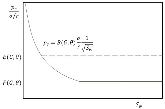
Figure 2.
Schematic of local capillary pressure function for variable wetting phase saturation.
2.4. Solution Scheme and Boundary Conditions
The solution scheme follows the IMPES algorithm. Firstly, Equation (8a,b) are combined and discretized to yield the implicit pressure equation as
where the local capillary pressure is treated in an explicit form (using the value from current time step ); i.e., .
After solving the pressure equations, the next step is to update the saturation explicitly using Equation (8a) a in discretized form:
Setting the maximum time step size for every time step interval is necessary to ensure that the solution scheme is stable. Here, we only allow a single pore body to be filled by the wetting phase for every step. The maximum time step size estimation from the current step cannot ensure the stability of the calculation of the next step due to the severe nonlinearity of this problem. This instability issue can be prevented by rechecking the maximum water saturation changing at the step. If this is less than unity, the calculation proceeds to the next step ; otherwise, the water saturation at the step is recalculated using a smaller time step size. The details can be found in the work by Aziz and Settari [45]. After obtaining the saturation field, the capillary pressure is updated; then, the calculation proceeds until the preset maximum time. Moreover, the throats are treated explicitly by applying the Equations (8) and (15), which significantly reduces the nonlinearity of the conductivity of non-wetting phase.
The boundary conditions for spontaneous imbibition are set as follows:
where the initially capillary pressure of every pore element is set as the maximum pressure .
3. Dynamic Pore-Scale Network Modeling of Water Imbibition in Shale and Tight Formations
Firstly, the pore network of Barnett shale is generated using the truncated lognormal distribution of Equation (1), and the single-phase flow simulation is validated. Moghaddam and Jamiolahmady [46] presented the experimental study of the apparent gas permeability of Barnett shale samples; the corresponding pore-throat distributions were obtained from high-pressure mercury injection capillary pressure (HPMICP) experiments. We use Equation (1) to fit the experimental throat radius distribution data of HPMICP, and the mean, minimum and maximum of the throat radii are 6.2, 1 and 50 nanometers, respectively. Since the pore throat aspect ratio is non-trivial to be obtained for shale, the value is set as 1.7 following the works of Valvatne and Blunt [22]. For gas flow in shale and tight formations, the smaller the pore size, the more important the effect of a gas–solid collision; therefore, the corresponding non-Darcy effect needs to be considered. After considering the gas non-Darcy flow (the details are provided in our previous work [47]) for every pore element, the calculated apparent gas permeability and experimentally measured data show a good match, as shown in Figure 3, which demonstrates that the generated network is representative for Barnett Shale, which forms the foundation for the following two-phase flow simulation.
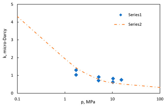
Figure 3.
Apparent gas permeability of a Barnett shale sample: experiment and pore network modeling.
Using the obtained pore network for Barnett shale, the initialization is conducted by setting every pore and throat element to have the local capillary pressure . Then, boundary conditions (Equation (17a) through (17d)) are applied in our dynamic pore network model, and the upper and lower boundaries are set as periodic. The water imbibition process can then be simulated directly within this proposed dynamic pore network model representing Barnett shale. Figure 4 shows the effect of the network size on the simulated spontaneous imbibition recovery with respect to time. We can see that a size of 20 × 60 is sufficient to capture the accuracy and efficiency for the following studies. The water saturation profiles of the water imbibition process are shown in Figure 5, where the average water saturation equals 0.2239. Note that the contact angle is set as 60° as the advancing contact angle is larger than the intrinsic contact angle due to the hysteresis effect [48]. All the mentioned conditions are set as the base case.
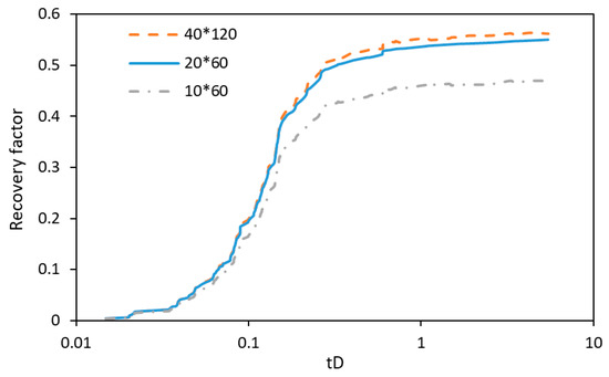
Figure 4.
Effect of pore network size on the simulated imbibition recovery.
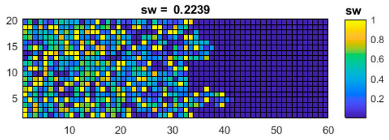
Figure 5.
Water saturation profiles of the water imbibition process using the proposed dynamic pore network model with an average water saturation equal to 0.2239.
Generally, a mixed wettability is assumed for shale and tight formations. Here, we considered mixed wet conditions for Barnett shale. We assigned three types of mixed wet conditions—30% oil-wet, 50% oil-wet and 70% oil-wet—as shown in Figure 6. The corresponding spontaneous water imbibition-induced oil recoveries are shown in Figure 7 for dimensionless time , where is the unit conversion factor, which is equal to 0.018849 if is in minutes, in md, in decimal, in , in cp, and L is a characteristic length in cm [49]; we follow the same units here. According to the figure, with the increasing proportion of oil-wet pores, the imbibition rate and recovery factor decrease dramatically. The results indicate that wettability dominates the water imbibition characteristics.
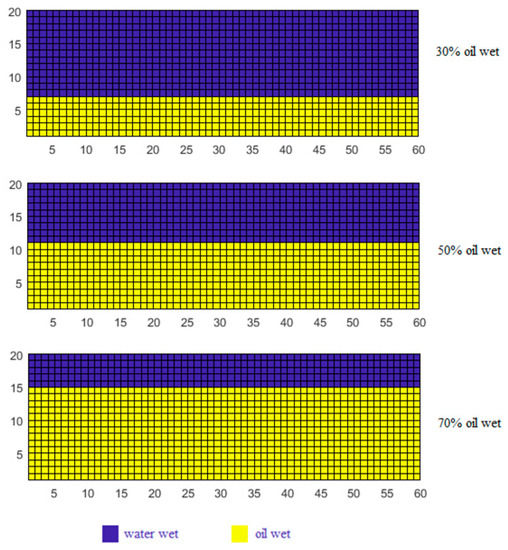
Figure 6.
Three types of mixed wet conditions.
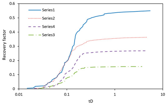
Figure 7.
Spontaneous imbibition recovery with respect to dimensionless time for different wettability distributions.
The existence of micro-fractures is considered in this work to investigate their effect on water imbibition, as natural and hydraulic fractures are presented within shale and tight formations. Four lines of micro-fractures are assigned within the Barnett shale pore network, and the pore radius is set as 20 nanometers (c.f. Figure 8), which is 3.23 times the mean radius of the Barnett shale matrix; therefore, the micro-fracture permeability is approximately 10 times that of the matrix permeability. The corresponding imbibition recovery with respect to dimensionless time is shown in Figure 9. With the existence of micro-fractures, the imbibition rate increases significantly while the final recovery remains similar. The micro-factures contribute to the conductance of the pore network instead of the pore volume, and the increase of conductance increases the imbibition rate but not the final recovery, as the final recovery is controlled by the capillarity of the matrix pores and throats.

Figure 8.
Schematic of micro-fracture distributions in the pore network.
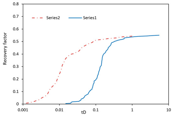
Figure 9.
Water imbibition recovery factor with and without micro-fractures.
Based on the above analysis, the simulated imbibition recovery factor with respect to dimensionless time is compared with the laboratory experimental work of Barnett shale samples by Morsy and Sheng [16]. The corresponding results are shown in Figure 10. Both the effects of wettability and micro-fractures are considered to fit the experimental data. Mixed wettability for Barnett shale is found within the fitting process. Since micro-fractures are observed in the imbibition experiments, the characteristic length is reduced significantly. In the fitting results, the effective characteristic length of Barnett shale samples is approximately several millimeters, and the fraction of oil-wet pores ranges from 70% to 50%.
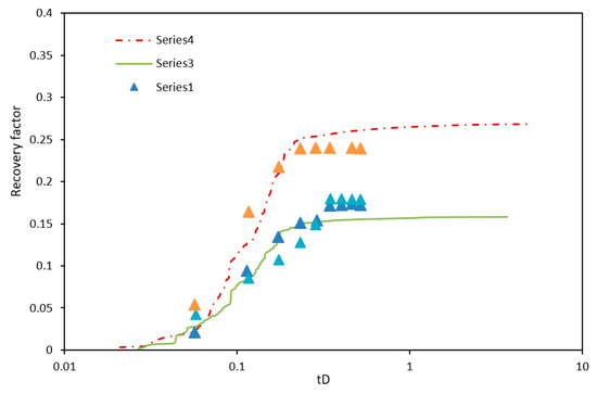
Figure 10.
Imbibition recovery factors of Barnett shale: pore network modeling and experiments [16].
Moreover, the effects of the initial maximum capillary pressure and the viscosity of the non-wetting phase on water imbibition are studied in this work, and the corresponding results are shown in Figure 11 and Figure 12. According to the figures, when the initial capillary pressure increases and the non-wetting phase viscosity decreases, the corresponding imbibition rates increase. However, the final imbibition recovery factor tends to be similar, which is because the water imbibition process is a capillary-dominated flow and the recovery factor is controlled by capillarity, which is affected by pore shape, aspect ratio, contact angle, etc. Therefore, the viscous forces in the reservoir conditions increase the imbibition rates but not the final recovery factor.
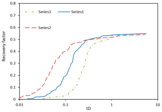
Figure 11.
Spontaneous imbibition with different initial maximum capillary pressures.
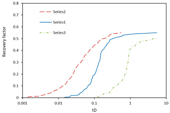
Figure 12.
Spontaneous imbibition with different non-wetting phase viscosities.
To further investigate the capillarity effect on the water imbibition of Barnett shale, the following sensitivity studies are conducted: the determination of the pore throat aspect ratio, contact angle and shape factor of the cross-area. The corresponding results for the water imbibition recovery factor with respect to dimensionless time are shown in Figure 13, Figure 14 and Figure 15, respectively. A higher aspect ratio tends to increase the percentage of the non-wetting phase trapped by the snap-off effect, which increases the residual non-wetting phase saturation and hence the final recovery factor (c.f. Figure 13). When the contact angle and cross-area shape factor decrease, leading to an increase of capillary pressure, the imbibition rate increases at the beginning. However, the final recovery factor decreases slightly (c.f. Figure 13 and Figure 14) because snap-off tends to occur more frequently with a lower contact angle and shape factor, as shown in Equation (13).
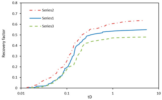
Figure 13.
Water imbibition recovery factor with different pore throat aspect ratios.
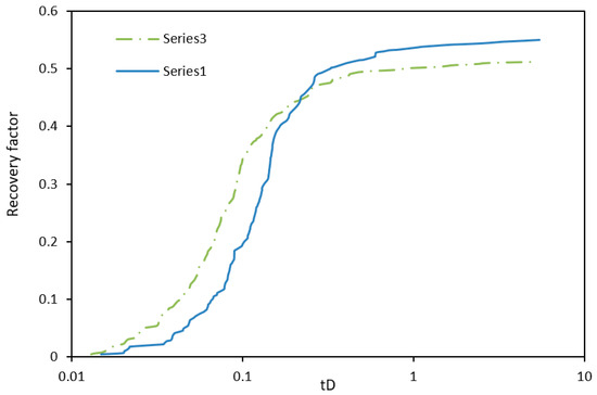
Figure 14.
Water imbibition recovery factor with different contact angles.
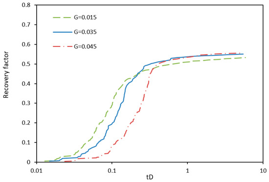
Figure 15.
Water imbibition recovery factor with different shape factors.
4. Summary and Conclusions
In this paper, a dynamic pore network model is proposed, including the pore network generation, local capillary pressure function, conductance calculation and boundary conditions for water imbibition. The proposed model is applied to Barnett shale formations, and the corresponding laboratory imbibition experiments are matched using the dynamic established pore network model. Then, systematical sensitivity studies are conducted. According to the simulated results using our dynamic pore network model, wettability dominates the water imbibition characteristics. Besides this, the viscous effects including viscosity, initial capillary pressure and micro-fractures increase the imbibition rate, while the final recovery factor is controlled to a greater extent by the capillarity effect including the cross-area shape factor, contact angle and aspect ratio.
Author Contributions
X.W. proposed the model and did the simulation work under the supervision and help of J.J.S. All authors have read and agreed to the published version of the manuscript.
Funding
This work is supported by the Foundation of China Postdoctoral Science (2019M660933), Foundation of State Key Laboratory of Petroleum Resources and Prospecting (PRP/indep-4-1814) and the Opening Fund of Key Laboratory of Unconventional Oil & Gas Development (19CX05005A-3).
Conflicts of Interest
The authors declare no conflict of interest.
Nomenclature
| Cross-area of a pore element | |
| Local capillary pressure function coefficient | |
| Coefficient accounting extra resistance of wetting layers | |
| Coefficient of piston-like displacement | |
| Coefficient of snap-off | |
| Shape factor of cross-area | |
| Corner shape factor | |
| Absolute conductance of a pore element | |
| Relative conductance of a pore element | |
| Water saturation | |
| Capillary pressure | |
| The characteristic length of imbibition | |
| The perimeter of the cross-area of a pore element | |
| Pore body volume | |
| Phase pressure | |
| Pore or throat radius | |
| Half angle of the corners | |
| Contact angle | |
| Fluid viscosity | |
| Interfacial tension | |
| Porosity | |
| Time step size | |
| Dimensionless time for imbibition upscaling | |
| Superscript | |
| Non-wetting phase | |
| Wetting phase | |
| Current time step | |
| Next time step | |
| Subscript | |
| th pore element | |
| th pore element | |
| Connecting throat between th and th pore elements | |
References
- Shanley, K.W.; Cluff, R.M.; Robinson, J.W. Factors controlling prolific gas production from low-permeability sandstone reservoirs: Implications for resource assessment, prospect development, and risk analysis. AAPG Bull. 2004, 88, 1083–1121. [Google Scholar] [CrossRef]
- Shaoul, J.R.; van Zelm, L.F.; De Pater, C.J. Damage mechanisms in unconventional-gas-well Stimulation--a new look at an old problem. SPE Prod. Oper. 2011, 26, 388–400. [Google Scholar]
- Hirasaki, G.; Zhang, D.L. Surface chemistry of oil recovery from fractured, oil-wet, carbonate formations. SPE J. 2004, 9, 151–162. [Google Scholar] [CrossRef]
- Zhang, P.; Austad, T. Wettability and oil recovery from carbonates: Effects of temperature and potential determining ions. Colloids Surf. A Physicochem. Eng. Asp. 2006, 279, 179–187. [Google Scholar] [CrossRef]
- Sheng, J.J. Review of surfactant enhanced oil recovery in carbonate reservoirs. Adv. Pet. Explor. Dev. 2013, 6, 1–10. [Google Scholar]
- Wang, D.; Butler, R.; Zhang, J.; Seright, R. Wettability survey in Bakken shale with surfactant-formulation imbibition. SPE Reserv. Eval. Eng. 2012, 15, 695–705. [Google Scholar] [CrossRef]
- Alvarez, J.O.; Schechter, D.S. Wettability alteration and spontaneous imbibition in unconventional liquid reservoirs by surfactant additives. SPE Reserv. Eval. Eng. 2017, 20, 10117. [Google Scholar] [CrossRef]
- Sheng, J.J. What type of surfactants should be used to enhance spontaneous imbibition in shale and tight reservoirs? J. Pet. Sci. Eng. 2017, 159, 635–643. [Google Scholar] [CrossRef]
- Zhang, X.; Morrow, N.R.; Ma, S. Experimental verification of a modified scaling group for spontaneous imbibition. SPE Reserv. Eng. 1996, 11, 280–285. [Google Scholar] [CrossRef]
- Akin, S.; Schembre, J.M.; Bhat, S.K.; Kovscek, A.R. Spontaneous imbibition characteristics of diatomite. J. Pet. Sci. Eng. 2000, 25, 149–165. [Google Scholar] [CrossRef]
- Zhou, X.; Morrow, N.R.; Ma, S. Interrelationship of wettability, initial water saturation, aging time, and oil recovery by spontaneous imbibition and waterflooding. SPE J. 2000, 5, 199–207. [Google Scholar] [CrossRef]
- Morrow, N.R.; Mason, G. Recovery of oil by spontaneous imbibition. Curr. Opin. Colloid Interface Sci. 2001, 6, 321–337. [Google Scholar] [CrossRef]
- Fischer, H.; Morrow, N.R. Scaling of oil recovery by spontaneous imbibition for wide variation in aqueous phase viscosity with glycerol as the viscosifying agent. J. Pet. Sci. Eng. 2006, 52, 35–53. [Google Scholar] [CrossRef]
- Takahashi, S.; Kovscek, A.R. Spontaneous countercurrent imbibition and forced displacement characteristics of low-permeability, siliceous shale rocks. J. Pet. Sci. Eng. 2010, 71, 47–55. [Google Scholar] [CrossRef]
- Roychaudhuri, B.; Tsotsis, T.T.; Jessen, K. An experimental investigation of spontaneous imbibition in gas shales. J. Pet. Sci. Eng. 2013, 111, 87–97. [Google Scholar] [CrossRef]
- Morsy, S.; Sheng, J.J. Imbibition characteristics of the barnett shale formation. In Proceedings of the SPE Unconventional Resources Conference, The Woodlands, TX, USA, 1–3 April 2014. SPE-168984-MS. [Google Scholar]
- Lucas, R. Rate of capillary ascension of liquids. Kolloid Z 1918, 23, 15–22. [Google Scholar] [CrossRef]
- Li, K.; Horne, R. Characterization of Spontaneous Water Imbibition into Gas-Saturated Rocks. In Proceedings of the SPE/AAPG Western Regional Meeting, Long Beach, CA, USA, 19–22 June 2000. [Google Scholar]
- Cai, J.; Perfect, E.; Cheng, C.L.; Hu, X. Generalized modeling of spontaneous imbibition based on Hagen–Poiseuille flow in tortuous capillaries with variably shaped apertures. Langmuir 2014, 30, 5142–5151. [Google Scholar] [CrossRef]
- Mason, G.; Morrow, N.R. Developments in spontaneous imbibition and possibilities for future work. J. Pet. Sci. Eng. 2013, 110, 268–293. [Google Scholar] [CrossRef]
- Øren, P.E.; Bakke, S.; Arntzen, O.J. Extending predictive capabilities to network models. SPE J. 1998, 3, 324–336. [Google Scholar] [CrossRef]
- Valvatne, P.H.; Blunt, M.J. Predictive pore-scale modeling of two-phase flow in mixed wet media. Water Resour. Res. 2004, 40, W07406. [Google Scholar] [CrossRef]
- Behbahani, H.; Blunt, M.J. Analysis of imbibition in mixed-wet rocks using pore-scale modeling. SPE J. 2005, 10, 466–474. [Google Scholar] [CrossRef]
- Behbahani, H.S.; Di Donato, G.; Blunt, M.J. Simulation of counter-current imbibition in water-wet fractured reservoirs. J. Pet. Sci. Eng. 2006, 50, 21–39. [Google Scholar] [CrossRef]
- Wang, X.; Sheng, J.J. Spontaneous imbibition analysis in shale reservoirs based on pore network modeling. J. Pet. Sci. Eng. 2018, 169, 663–672. [Google Scholar] [CrossRef]
- Wang, X.; Sheng, J.J. A self-similar analytical solution of spontaneous and forced imbibition in porous media. Adv. Geo-Energ. Res. 2018, 2, 260–268. [Google Scholar] [CrossRef]
- Nguyen, V.H.; Sheppard, A.P.; Knackstedt, M.A.; Pinczewski, W.V. The effect of displacement rate on imbibition relative permeability and residual saturation. J. Pet. Sci. Eng. 2006, 52, 54–70. [Google Scholar] [CrossRef]
- Blunt, M.J. Multiphase Flow in Permeable Media: A Pore-Scale Perspective; Cambridge University Press: Cambridge, UK, 2017. [Google Scholar]
- Sheng, Q.; Thompson, K. A unified pore-network algorithm for dynamic two-phase flow. Adv. Water Resour. 2016, 95, 92–108. [Google Scholar] [CrossRef]
- Blunt, M.J.; Scher, H. Pore-level modeling of wetting. Phys. Rev. E 1995, 52, 6387. [Google Scholar] [CrossRef]
- Hughes, R.G.; Blunt, M.J. Pore scale modeling of rate effects in imbibition. Transp. Porous Media 2000, 40, 295–322. [Google Scholar] [CrossRef]
- Idowu, N.A.; Blunt, M.J. Pore-scale modelling of rate effects in waterflooding. Transp. Porous Media 2010, 83, 151–169. [Google Scholar] [CrossRef]
- Aghaei, A.; Piri, M. Direct pore-to-core up-scaling of displacement processes: Dynamic pore network modeling and experimentation. J. Hydrol. 2015, 522, 488–509. [Google Scholar] [CrossRef]
- Aker, E.; Måløy, K.J.; Hansen, A.; Batrouni, G.G. A two-dimensional network simulator for two-phase flow in porous media. Transp. Porous Media 1998, 32, 163–186. [Google Scholar] [CrossRef]
- Al-Gharbi, M.S.; Blunt, M.J. Dynamic network modeling of two-phase drainage in porous media. Phys. Rev. E 2005, 71, 016308. [Google Scholar] [CrossRef] [PubMed]
- Tørå, G.; Øren, P.E.; Hansen, A. A dynamic network model for two-phase flow in porous media. Transp. Porous Media 2012, 92, 145–164. [Google Scholar] [CrossRef]
- Khayrat, K. Modeling Hysteresis for Two-Phase Flow in Porous Media: From Micro to Macro Scale. Ph.D. Thesis, ETH Zurich, Zurich, Switzerland, 2016. [Google Scholar]
- Joekar-Niasar, V.; Hassanizadeh, S.M.; Dahle, H.K. Non-equilibrium effects in capillarity and interfacial area in two-phase flow: Dynamic pore-network modelling. J. Fluid Mech. 2010, 655, 38–71. [Google Scholar] [CrossRef]
- Khayrat, K.; Jenny, P. A multi-scale network method for two-phase flow in porous media. J. Comput. Phys. 2017, 342, 194–210. [Google Scholar] [CrossRef]
- Mason, G.; Morrow, N.R. Capillary behavior of a perfectly wetting liquid in irregular triangular tubes. J. Colloid Interface Sci. 1991, 141, 262–274. [Google Scholar] [CrossRef]
- Ransohoff, T.C.; Radke, C.J. Laminar flow of a wetting liquid along the corners of a predominantly gas-occupied noncircular pore. J. Colloid Interface Sci. 1988, 121, 392–401. [Google Scholar] [CrossRef]
- Bakke, S.; Øren, P.E. 3-D pore-scale modeling of sandstones and flow simulations in the pore networks. SPE J. 1997, 2, 136–149. [Google Scholar] [CrossRef]
- Patzek, T.W. Verification of a complete pore network simulator of drainage and imbibition. In Proceedings of the SPE/DOE Improved Oil Recovery Symposium, Tulsa, OK, USA, 3–5 April 2000. [Google Scholar]
- Andersen, P.Ø.; Skjæveland, S.M.; Standnes, D.C. A Novel Bounded Capillary Pressure Correlation with Application to Both Mixed and Strongly Wetted Porous Media. In Proceedings of the SPE Abu Dhabi International Petroleum Exhibition & Conference, 13–16 November 2017. SPE-188291-MS. [Google Scholar]
- Aziz, K.; Settari, A. Petroleum Reservoir Simulation; Chapman & Hall: London, UK, 1979. [Google Scholar]
- Moghaddam, R.N.; Jamiolahmady, M. Fluid transport in shale gas reservoirs: Simultaneous effects of stress and slippage on matrix permeability. Int. J. Coal Geol. 2016, 163, 87–99. [Google Scholar] [CrossRef]
- Wang, X.; Sheng, J.J. Pore network modeling of the non-Darcy flows in shale and tight formations. J. Pet. Sci. Eng. 2018, 163, 511–518. [Google Scholar] [CrossRef]
- Morrow, N.R. The effects of surface roughness on contact: Angle with special reference to petroleum recovery. J. Can. Pet. Technol. 1975, 14, 42–53. [Google Scholar] [CrossRef]
- Ma, S.; Zhang, X.; Morrow, N.R. Influence of fluid viscosity on mass transfer between rock matrix and fractures. J. Can. Pet. Technol. 1999, 38, 25–30. [Google Scholar] [CrossRef]
© 2020 by the authors. Licensee MDPI, Basel, Switzerland. This article is an open access article distributed under the terms and conditions of the Creative Commons Attribution (CC BY) license (http://creativecommons.org/licenses/by/4.0/).