Numerical Modeling and Performance Evaluation of Standing Wave Thermoacoustic Refrigerators with a Multi-Layered Stack

Abstract

Thermoacoustic refrigerators have huge potential to replace conventional refrigeration systems as an alternative clean refrigeration technology. These devices utilize conversion of acoustic power and heat energy to generate the desired cooling. The stack plays a pivotal role in the performance of Standing Wave Thermoacoustic Refrigerators (SWTARs), as the heat transfer takes place across it. Performance of stacks can be significantly improved by making an arrangement of different materials inside the stack, resulting in anisotropic thermal properties along the length. In the present numerical study, the effect of multi-layered stack on the refrigeration performance of a SWTAR has been evaluated in terms of temperature drop across the stack, acoustic power consumed and device Coefficient of Performance (COP). Two different aspects of multi-layered stack, namely, different material combinations and different lengths of stacked layers, have been investigated. The combinations of four stack materials and length ratios have been investigated. The numerical results showed that multi-layered stacks produce lower refrigeration temperatures, consume less energy and have higher COP value than their homogeneous counterparts. Among all the material combinations of multi-layered stack investigated, stacks composed of a material layer with low thermal conductivity at the ends, i.e., RVC, produced the best performance with an increase of 26.14% in temperature drop value, reduction in the acoustic power consumption by 4.55% and COP enhancement of 5.12%. The results also showed that, for a constant overall length, an increase in length of side stacked material layer results in an increase in values of both temperature drop and COP.

Highlights

• Numerical modeling of multi-layered stack inside standing wave thermoacoustic refrigerator is conducted.
• Multi-layered stack is composed of an arrangement of different materials inside a stack and the effect of various multi-layered stack material and length combinations is analyzed.
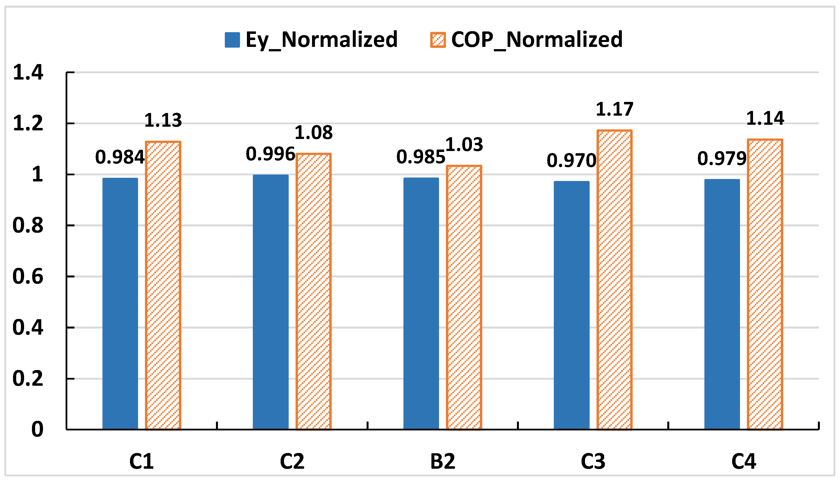
• Celcor based RVC stacks showed an improvement of 26.14%, 5.12% and 4.55% in terms of temperature drop, Coefficient of Performance (COP) and total energy flux, respectively.
• Addition of layer of insulative material at stack ends has a beneficial effect on the refrigeration performance.

1. Introduction

The excessive emission of the conventional Chlorofluorocarbons (CFCs) refrigerants has caused severe damage to the Earth’s stratospheric protective ozone layer. In order to mitigate the excessive damage of the ozone layer, the conventional refrigeration system needs to be replaced by an environmentally friendly refrigeration system. Thermoacoustic refrigeration systems could be one of the possible options to replace the conventional refrigeration systems due to the absence of the refrigerant for cooling process. Standing Wave Thermo-Acoustic Refrigerators (SWTARs) operate by utilizing the interaction of thermal and acoustic fields between compressible oscillating fluid and solid plates that results in a net pumping of heat across the solid porous media [1]. These devices utilize noble gases, involve no moving parts and can also be driven by waste [2,3,4] or solar heat [5,6]. Thus, SWTAR is an attractive candidate to replace conventional refrigerators due to its minimal operating costs and very low environmental impact [1]. However, low overall efficiency of SWTAR is the primary hindrance in the commercial acceptance of this technology [7].

An excellent discussion of the theoretical framework governing the behavior inside Thermo-Acoustic Devices (TAD) is provided by Swift [1,8]. The governing equations are based on 1-D linear thermoacoustic theory introduced by Rott [9]. Linear model can be beneficial for design and optimization of thermoacoustic systems [10]. However, the linear model is simplified based on certain major assumptions, i.e., steady state flow, low pressure amplitude, linearized wave equation etc. [1], and cannot account for transient and complex non-linear phenomena [11]. Higher order numerical models are, therefore, inevitable for modeling various nonlinear loss mechanisms, power rating and accurate performance prediction of these devices [12].

Numerical modeling of SWTAR is computationally expensive due to disparity in the length scales of different components. Hence, numerical studies of SWTAR have utilized simplified computational domains for numerical simulations, i.e., modeling a single stack space with truncated domain and no heat exchangers, denoted as Thermoacoustic Couple (TAC) [13]. Cao et al. [14] numerically computed the energy and heat fluxes across a TAC of a short stack with isothermal conditions. Worlikar et al. [15,16] utilized similar TAC domain to develop low Mach number approximation of fully compressible Navier–Stokes equations. They successfully captured vortices formation at stack edges by solving stream-function vorticity equation. Ishikawa and Mee [11] extended the work of Cao et al. [14] for long stacks and analyzed the effect of plate spacing on device performance. Marx and Benon [17,18,19] calculated the mean velocity field, temperature distribution and temperature distortion across the stacks using a single stack model. In a recent study, Mergen et al. [20] analyzed the effect of variation in computational domain length on the performance simulation of SWTAR using similar TAC domain proposed by Cao et al. [14]. All the above studies modeled the stack with zero thickness and thus are unable to incorporate the effect of stack material properties on the device performance.

One of the first attempts to numerically model and analyze the performance of SWTAR with stacks having a non-zero thickness is made by Zoontjens et al. [21]. In their work, flow and energy fields are simulated inside a single stack domain using a hypothetical stack with finite thickness and thermal conductivity. Abd EI-Rahman and Abdel Rahman [22] utilized a single stack domain to model a high frequency SWTAR with fiberglass laminate stack. They presented a fully implicit time integration algorithm that is unconditionally stable with respect to the time increment size. The transient simulations reported a three times increase in the acoustic power consumption of a stack with a 40% reduction in its spacing. In a subsequent study [23], a 3-D model of a single square stack is analyzed numerically for higher amplitude conditions and it is observed that the flow adheres to 1-D linear theory even up to drive ratios of 2%. The nonlinear vortices are localized at the stack ends and are suppressed quickly when compared to 2-D flow modeling.

A more comprehensive computational domain, comprising of both the heat exchangers and stack plate, is important for accurate performance simulation, evaluation of Coefficient of Performance (COP) and successful operation of the apparatus [24]. It has been utilized in few recent studies for the performance prediction of SWTAR. Low Mach number 2-D numerical model is developed by Nehar and Hireche [25] to analyze the effect of the blockage ratio between stack and heat exchangers. The combined length of the heat exchangers and stack is assumed to be less than the wavelength. It is concluded that higher the heat exchangers plate interspacing, higher is the refrigeration efficiency. Rahpiema and Ebrahimi [26] analyzed the performance of SWTAR for variation in the stack geometric and thermo-physical properties, using TAC enclosing both heat exchangers and stack. It was concluded that, for a fixed temperature difference across stack, lower cooling temperatures and higher COPs can be achieved by reducing thickness and thermal conductivity of the stack plates. Fatimah and Jaworski [27] analyzed the temperature and velocity profiles inside parallel heat exchangers of standing wave thermoacoustic system using a detailed 2-D Computational Fluid Dynamics (CFD) model. The model was able to capture the flow field asymmetries and streaming effects present in the oscillatory flows. In a subsequent study [28], transition conditions from laminar to turbulent in oscillatory flows across parallel plate heat exchangers are discussed numerically. A new range for critical Reynold number is presented and it is reported that flow transition can take place for its value between 70 and 100. More recently, Rogoziński and Nowak developed a 2-D numerical model for dual thermoacoustic engine with moving piston [29].

Performance of thermoacoustic devices can be significantly improved by enhancing the power density of stack. For the said purpose, researchers have devoted considerable effort, both experimental and numerical, to enhance the stack performance by exploring novel concepts. Some efforts include usage of wet stack or regenerator [30,31], random stack configuration [32], converging stack design [33] and various stack plate edge profiles/shapes [34]. Recently, Auriemma et al. conducted a numerical study to compare the performance of stacks with different geometries for building applications [35].

The design of stack in Standing-wave thermoacoustic devices is a challenging task and involves a trade-off among many issues. One possible way to achieve higher performance is to have an arrangement of different materials inside the stack resulting in anisotropic thermal properties along the stack length. As suggested by Zolpakar et al. [36] in their review, inclusion of non-isotropic material might improve the performance of the stack. For the case of SWTAR, variation of thermal properties along the stack length may result in reduction of negative heat/energy transfers taking place between the fluid parcel and solid plate, thus reducing the inherent irreversibility associated with the stack materials [1]. The arrangement can be realized by having a multi-layered stack composed of alternative insulating and conductive materials. To the authors’ knowledge, the only work that considered the arrangement of different materials inside the stack, for the performance evaluation of standing wave thermoacoustic devices, is the experimental work conducted by Tasnim [37]. In that work, heterogeneous stacks, composed of Aluminum, RVC and Celcor, are inserted in a simple standing-wave thermoacoustic heat pump. Elementary results for various configurations in terms of temperature drop illustrated that heterogeneous stacks have better cooling performance than the homogeneous stack. Based on the temperature profiles obtained at the stack ends, the heterogeneous stack combinations also showed reduced return diffusive heat transfer, thus increasing their efficiency.

In light of this information, there might be a possibility to improve the performance of the standing wave thermoacoustic devices by deliberately varying the thermal properties inside the stack. In the present study, a detailed and systematic evaluation of various aspects of a multi-layered stack on the performance of SWTAR have been conducted numerically. A comprehensive 2-D numerical model, with both the stack and the heat exchangers, consisting of a representative computational domain, has been utilized for investigation. The effects of various multi-layered stack material combinations and effect of variation in length of layered materials has been analyzed in terms of temperature difference achieved by the refrigerator, energy flux consumed by the stack and COP attained by the SWTAR.

2. Mathematical Background

The numerical model is based on Navier–Stokes, continuity and energy equations. Since the developed numerical model is two-dimensional, the body forces are neglected for both the fluid and solid domains. Complete thermoacoustic phenomenon is analyzed numerically for a fully developed compressible fluid domain by solving continuity, Navier–Stokes and energy equations given by

$$\frac{\partial \rho }{\partial t}+\frac{\partial (\rho u)}{\partial x}+\frac{\partial (\rho v)}{\partial y}=0$$

(1)

$$\frac{\partial (\rho u)}{\partial t}+ \nabla .(\rho u\overrightarrow{V})=-\frac{\partial p}{\partial x}+\frac{\partial {\sigma }_{xx}}{\partial x}+\frac{\partial {\sigma }_{yx}}{\partial y}$$

(2)

$$\frac{\partial (\rho v)}{\partial t}+ \nabla .(\rho v\overrightarrow{V})=-\frac{\partial p}{\partial y}+\frac{\partial {\sigma }_{xy}}{\partial x}+\frac{\partial {\sigma }_{yy}}{\partial y}$$

(3)

$$\begin{array}{cc}\hfill \frac{\partial }{\partial t}\left[\rho \left(ϵ+\frac{V^2}{2}\right)\right]& +\nabla .\left[\rho \left(h+\frac{V^2}{2}\right)\overrightarrow{V}\right]\hfill \\ & =\rho \dot{q}+\frac{\partial }{\partial x}\left(k\frac{\partial T}{\partial x}\right)+\frac{\partial }{\partial y}\left(k\frac{\partial T}{\partial y}\right)-\frac{\partial \left(up\right)}{\partial x}-\frac{\partial \left(vp\right)}{\partial y}+\frac{\partial \left(u{\sigma }_{xx}\right)}{\partial x}+\frac{\partial \left(u{\sigma }_{yx}\right)}{\partial y}\hfill \\ & +\frac{\partial (v{\sigma }_{xy})}{\partial x}+\frac{\partial \left(v{\sigma }_{yy}\right)}{\partial y}\hfill \end{array}$$

(4)

For the solid domain, only transient heat conduction equation is solved and the governing equation is given by:

$$\rho C_p\frac{\partial T}{\partial t}=k\left(\frac{{\partial }^{2}T}{\partial x^2}+\frac{{\partial }^{2}T}{\partial y^2}\right)+S$$

(5)

In Equations (1)–(5), $\rho$,$u$, $v$, $\overrightarrow{V}$, $p$, $ϵ$,$h$, $V$, $\dot{q}$, $k$, $C_p$, $T$ and $S$ are density, x-velocity, y-velocity, velocity vector, pressure, internal energy, specific enthalpy of fluid, velocity magnitude, heat transfer rate, thermal conductivity coefficient, constant pressure heat capacity, temperature and heat source, respectively. Furthermore, ${\sigma }_{ij}$ is a stress tensor where i specifies the stress component’s direction and j specifies the surface orientation on which stress is acting.

For problems involving convection heat transfer, energy flux density ($\dot{e}$) is a useful parameter for visualizing the amount and direction of energy transfer. The x and y components of $\dot{e}$ can be represented by following equations:

$${\dot{e}}_x=\rho u\left(\frac{1}{2}{V}^2+h\right)-k\frac{\partial T}{\partial x}-\left(u{\sigma }_{xx}+v{\sigma }_{yx}\right)$$

(6)

$${\dot{e}}_y=\rho v\left(\frac{1}{2}{V}^2+h\right)-k\frac{\partial T}{\partial y}-\left(u{\sigma }_{xy}+v{\sigma }_{yy}\right)$$

(7)

and viscous stress tensors, ${\sigma }_{ij}$, in the above equations are defined as

$${\sigma }_{xx}=\mu \frac{2}{3}\left[2\frac{\partial u}{\partial x}-\frac{\partial v}{\partial y}\right]$$

(8)

$${\sigma }_{yy}=\mu \frac{2}{3}\left[2\frac{\partial v}{\partial y}-\frac{\partial u}{\partial x}\right]$$

(9)

$${\sigma }_{xy}={\sigma }_{yx}=\mu \left[\frac{\partial u}{\partial y}+\frac{\partial v}{\partial x}\right]$$

(10)

where $\mu$ is the dynamic viscosity. Acoustic power applied at the inlet is given by relation

$${\dot{W}}_{ac}= \frac{1}{2}{P}_1{u}_1$$

(11)

where $P_1$ and $u_1$ are the amplitudes of oscillating pressure and velocity, respectively. Heat flux across the cold and hot heat exchangers is calculated by using the equation:

$$\dot{q}=-k\nabla T$$

(12)

All the fluid properties are changing periodically over one complete cycle of an acoustic wave. Thus, for a better evaluation, all major performance parameters are averaged over one acoustic cycle. The time-averaged values for ${\dot{e}}_y$,${\dot{W}}_{ac}$ and $\dot{q}$ can be calculated using the following formulation:

$$\langle {\dot{E}}_y\rangle {}_t= \frac{1}{\tau }{{\displaystyle \int }}_0^{\tau }{{\displaystyle \int }}_0^l{\dot{e}}_{y}dxdt$$

(13)

$${\langle \dot{W}\rangle }_t= \frac{1}{\tau }{{\displaystyle \int }}_0^{\tau }{{\displaystyle \int }}_y^{y_0}{\dot{W}}_{ac}dydt$$

(14)

$${\langle \dot{Q}\rangle }_t= \frac{1}{\tau }{{\displaystyle \int }}_0^{\tau }{{\displaystyle \int }}_0^l\dot{q}dxdt$$

(15)

The Coefficient of Performance (COP) of SWTAR is given by:

$$COP= \frac{\langle {\dot{Q}}_{CHx}\rangle {}_t}{{\langle \dot{W}\rangle }_t}$$

(16)

where $\langle {\dot{Q}}_{CHx}\rangle {}_t$ is the time-averaged heat flux across the cold heat exchanger (CHX) surface and ${\langle \dot{W}\rangle }_t$ is the time-averaged acoustic power applied at the inlet. A finite volume based numerical CFD model is utilized in the current study to analyze the performance of multi-layered stacks and the details of the model are presented in the next section.

3. Numerical Model

Figure 1a shows the computational domain used for the performance evaluation of the thermoacoustic system. It represents a truncated two-dimensional model of a quarter-wavelength resonator consisting of a stack and heat exchangers made of parallel plates. In the numerical model, the width of the stack plates is considered infinite. The left end of the resonator is closed while a predetermined acoustic power is supplied at the right open end.

To enable comparison and validation with previous studies, the numerical model of current work has utilized similar operating conditions and geometric parameters as proposed by Ishikawa and Mee [11]. Therefore, the resonator is filled with Helium gas at 10 kPa absolute pressure. Mean temperature of the device is 298 K and the speed of sound is maintained at 1008 m/s. The operating frequency of device is fixed at 100 Hz and the total length of resonator used is 2.52 m.

3.1. Model Space

The computational domain used in this work comprise of a thermoacoustic couple consisting of a single plate of stack, similar to the one proposed by Ishikawa and Mee [11] but with an expanded domain. The first expansion in the proposed domain was made by Zoontjens et al. [21] who considered the thickness of the stack to account for the solid conduction inside the stack. However, hypothetical material properties were assumed for stack material. The solution domain is further enhanced in the current work as shown in Figure 1b. It includes a hot heat exchanger (HHX) and a cold heat exchanger (CHX) placed at either sides of stack. Both the stack and heat exchangers are modeled as solids with non-zero thickness and realistic material properties. A gap of 0.5 mm is placed between each heat exchanger and the stack ends. For simplicity, the stack and heat exchangers are of the same height. Total length of the computational domain is 1/8 λ + 0.0085 λ where λ, is the wavelength of acoustic wave. The cold (right) end of stack is placed at a distance of 1/8 λ from the closed end. The height of the domain is (y₀ + th) where y₀ is half of stack spacing and th is half of the stack thickness. The left end of the domain is the closed end of the resonator while oscillating boundary conditions are applied at right end of domain. The stack plate can either be homogeneous stack made of a single layer of material or multi-layered stack made of different layers of materials stacked together. The multi-layered stack is divided into three layers, i.e., material layer at the right side (M_R), base material in the middle (B) and material layer at left side (M_L). Heat exchanger material is taken as copper and lengths of HHX and CHX are taken as 7 mm and 3.5 mm, respectively.

Eight different cases are run for comparison and evaluation of SWTAR performance under various configurations and combinations of multi-layered stacks. They include various combinations of stacked materials and different lengths of individual materials for some combinations. The overall length of stack (L_s) and height of the domain (y₀ + th) is kept constant in all simulations and are given by L_s = 253 mm and y₀ + th = 4.1 mm.

Two base materials, namely Celcor and Kapton, are considered in the analysis. Two different materials, namely RVC and Aluminum (Al), are considered for material layers M_R and M_L. Details of these cases are summarized in

Table 1. Details of all test cases simulated in the current study.

Sample Name	Stack Materials	Length in Terms of PD
		Base	MR	ML
B1	Celcor	11.0	-	-
B2	Kapton	11.0	-	-
C1/PD1	RVC, Celcor, RVC	9.0	1.0	1.0
C2	Al, Celcor, Al	9.0	1.0	1.0
C3	RVC, Kapton, RVC	9.0	1.0	1.0
C4	Al, Kapton, Al	9.0	1.0	1.0
PD2	RVC, Celcor, RVC	7.0	2.0	2.0
PD3	RVC, Celcor, RVC	5.0	3.0	3.0

PD = 23 mm, δ_k = 2.4 mm, half stack spacing, y_o = 4 mm; half plate thickness, th = 0.1 mm; overall stack length, L_s = 253 mm.

. The simulation is carried out from the onset of process until the steady-state is reached while the temperature of HHX is kept fixed. As shown in Table 1, all the simulations can be categorized into three main groups. At first, two cases are run with homogeneous stacks consisting of base materials only, comprising the first group with prefix B. The second group, having prefix C, consists of four different combinations of base and side stacked materials. The combinations are made such that alternating layers of stacks act as conducting and insulating materials inside the stack. A third group, with prefix PD, analyzes the effect of varying the length of different layers on the performance of the device. For said purpose, the length of the stacked materials at either side is varied as a multiple of particle displacement (PD) and base material length are adjusted to maintain the total length of the stack at 11PD.

3.2. Boundary and Operating Conditions

The conditions applied at each boundary of the computational domain are defined as:

$\begin{array}{c}u=0\\ v=0\\ \frac{dT}{dx}=0\end{array}\}$ at closed end.

$\begin{array}{c}\frac{du}{dy}=0\\ v=0\\ \frac{dT}{dx}=0\end{array}\}$ at fluid symmetry boundaries.

$\frac{dT}{dy}=0\}$ at solid symmetry boundaries

$\begin{array}{c}u=0\\ v=0\\ T_{fluid}=T_{solid}\end{array}\}$ at surface of solids.

The oscillatory boundary requires special treatment where standing wave conditions corresponding to an open end need to be implemented at the truncated domain. The pressure (P), temperature (T) and velocity (u) at oscillating end are given by:

$$P=P_m+Re\left\{P_1{e}^{i\omega t}\right\}$$

(17)

$$u=Re\left\{u_1{e}^{i\omega t}\right\}$$

(18)

$$T=T_m+Re\left\{T_1{e}^{i\omega t}\right\}$$

(19)

where P₁, T₁ and u₁ represent the first order amplitudes of oscillating pressure, temperature and velocity, respectively, and Re{ } represents the real part. T_m and P_m are mean temperature and pressure. Time dependence of all the parameters is given by $e^{i\omega t}$ term where ω is the angular frequency given by ω = 2πf and f is the normal frequency. P₁, u₁ and T₁ for a standing wave are further defined as

$$P_1=P_A\cos \left(kx\right)$$

(20)

$$u_1=-i\frac{P_A}{{\rho }_{m}a}\sin \left(kx\right)$$

(21)

$$T_1=\frac{P_A}{{\rho }_m{C}_p}\cos \left(kx\right)$$

(22)

where P_A is the pressure amplitude at pressure antinode, k is the wave number given by $2\pi /\lambda$, ${\rho }_m$ is the mean density, a is the speed of sound and $C_p$ is the specific heat at constant pressure. Thus, the finalized form of the equations applied for oscillatory boundary conditions at the right end of the domain are given by

$$P=P_m+P_A\cos \left(k{x}_{OS}\right)\cos \left(\omega t\right)$$

(23)

$$u_1=\frac{P_A}{{\rho }_{m}a}\sin \left(k{x}_{OS}\right)\sin \left(\omega t\right)$$

(24)

$$T=T_m+\frac{P_A}{{\rho }_m{C}_p}\cos \left(k{x}_{OS}\right)cos\left(\omega t\right)$$

(25)

where $x_{OS}$ is the location of the oscillating boundary.

Zero initial conditions are assumed at the start of all test cases, as follows:

$\begin{array}{c}u=0\\ v=0\\ T=T_m\end{array}\}$ at t = 0, at all x and y cells.

3.3. Material Properties

Helium gas is selected as the working fluid. The operating conditions and gas properties common to all simulations are summarized in

Table 2. Operating conditions and properties common to all simulations.

Property	Value	Unit
Working fluid	Helium	-
Mean Temperature, Tm	298	K
Mean pressure, Pm	10	kPa
Operating frequency, f	100	Hz
Oscillating pressure amplitude, PA	170	Pa
Drive Ratio, DR = PA/Pm	1.7	%
Wavelength, λ	10.08	m
HHX’s temperature (constant)	298	K
Gas properties:
Reference thermal conductivity, $k^{\prime }$	0.152	W/m·K
Reference dynamic viscosity, ${\mu }^{\prime }$	1.98 × 10−5	kg/m·s
Specific heat capacity, Cp	5190	J/kg·K
Prandtl no., σ	0.69	-

. The stack elements are modeled using solid materials with constant properties and the values considered for all simulations are tabulated in

Table 3. Properties of various solid materials used in simulations.

Material	Cp (J/kg·K)	k (W/m·K)	ρ (kg/m3)
Celcor	1000	1.46	2300
Kapton	1090	0.12	1420
RVC	1260	0.033	49.5
Al	895	5.8	216
Copper	385	400	8960

.

The thermal penetration depth (δ_k) and particle displacement length, (PD) are defined as:

$${\delta }_k= \sqrt{2k_f/{\rho }_m{C}_p\omega }$$

(26)

$$PD=2u_1/\omega$$

(27)

Based on the values given in Table 2, the calculated values of δ_k and PD are 2.3 mm and 24 mm, respectively.

The working fluid (Helium) is assumed as an ideal gas and its density is governed by the equation of state. Viscosity and thermal conductivity of Helium is modeled using power law, as proposed by Ishikawa and Mee [11], with n = 0.647. Thus, dynamic viscosity and thermal conductivity are given by

$$\mu = {\mu }^{\prime }{\left(\frac{T}{T^{\prime }}\right)}^n$$

(28)

$$k= k^{\prime }{\left(\frac{T}{T^{\prime }}\right)}^n$$

(29)

where, $\mu , k$ are dynamic viscosity and thermal conductivity at temperature T of fluid, respectively, while ${\mu }^{\prime }$ and $k^{\prime }$ are dynamic viscosity and thermal conductivity at the reference temperature, $T^{\prime }$.

3.4. Numerical Implementation

A finite volume based numerical package, i.e., ANSYS Fluent, is used to perform the simulations. Double precision parallel computation with unsteady formulation is utilized for the analysis. Both flow and energy equations are solved for capturing the physical thermoacoustic phenomena while the conjugate heat transfer algorithm is utilized to model the heat transfer between the fluid and solid boundaries. For oscillatory flows inside the pipes, the transition of flow from laminar to turbulent is determined using the Stokes based critical Reynolds number and it is given by $R{e}_{cr}=2u_1/\sqrt{\nu \omega }$ where $u_{1 }$is the amplitude of oscillating velocity and $\nu$ is the kinematic viscosity of the fluid. The value of $R{e}_{cr}= 400$ was given by Merkli and Thomann [38] as the condition where the Stokes layer becomes unstable and flow transition takes place. As the Mach number of the current simulation setup is 0.01 and the $R{e}_{cr}$ is always below 400, turbulence is neglected and laminar flow conditions are assumed to prevail.

Pressure based solver with absolute velocity formulation is selected for the transient analysis. First order implicit scheme is used for temporal discretization, while spatial discretization is carried out using second order upwind schemes. For pressure interpolation, the high accuracy pressure staggering scheme (PRESTO) is selected, while Pressure Implicit with Splitting of Operators (PISO) is enabled for pressure velocity coupling.

Selection of appropriate time step is of utmost importance to ensure fast convergence and accurate capturing of the cyclic thermoacoustic refrigeration process. Thus, sufficient resolution of each waveform is ensured by selecting a fixed time step of 5 × 10⁻⁵ s for all simulations. As a result, every single oscillation period (τ) is captured in 200 time steps ($\Delta t= \tau /200$). The justification for the selection of this time step is presented as part of the mesh independence study in the following section. The maximum number of allowable iterations in each time step is 125. However, convergence is achieved in between 25 to 30 iterations with the selected time step.

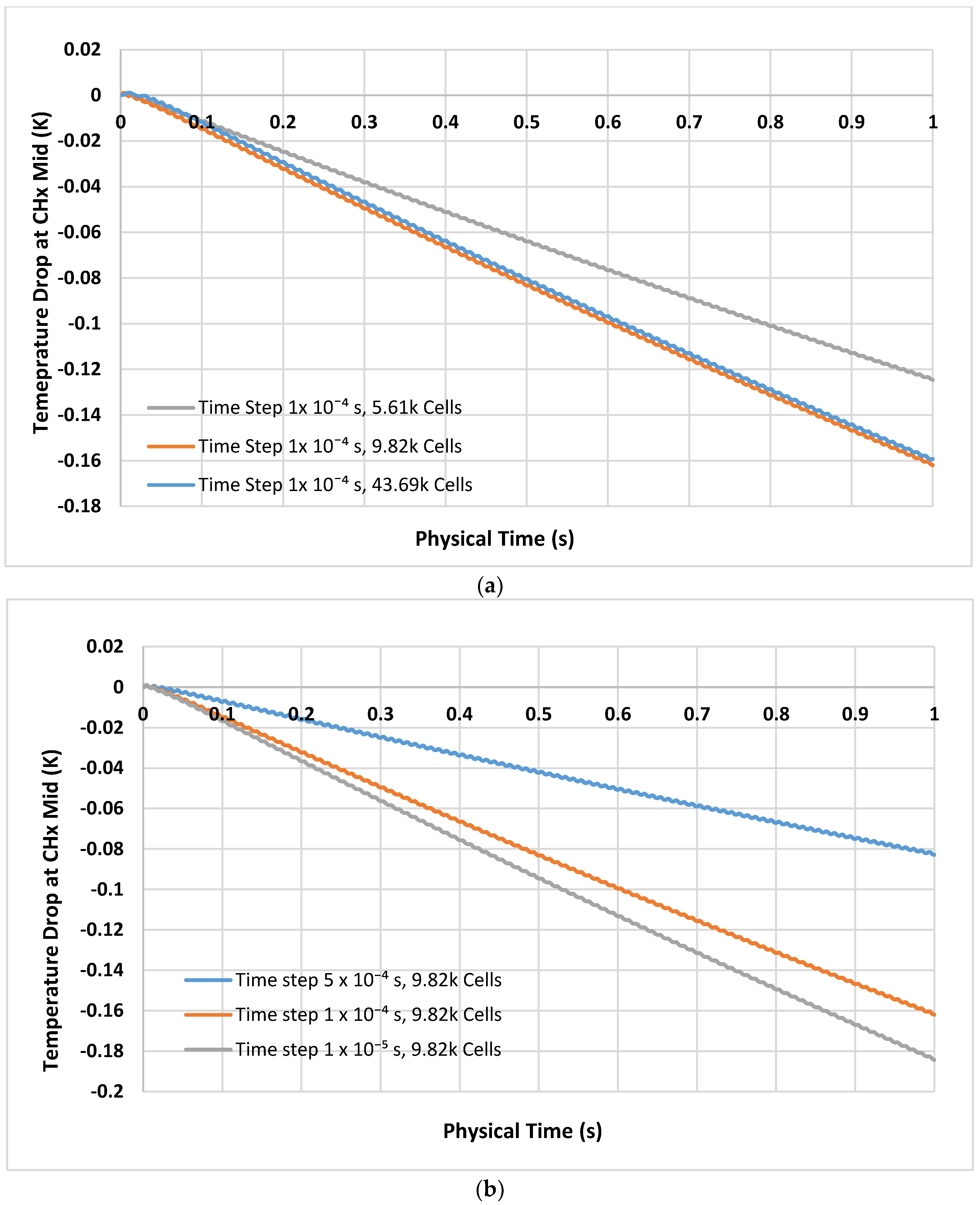
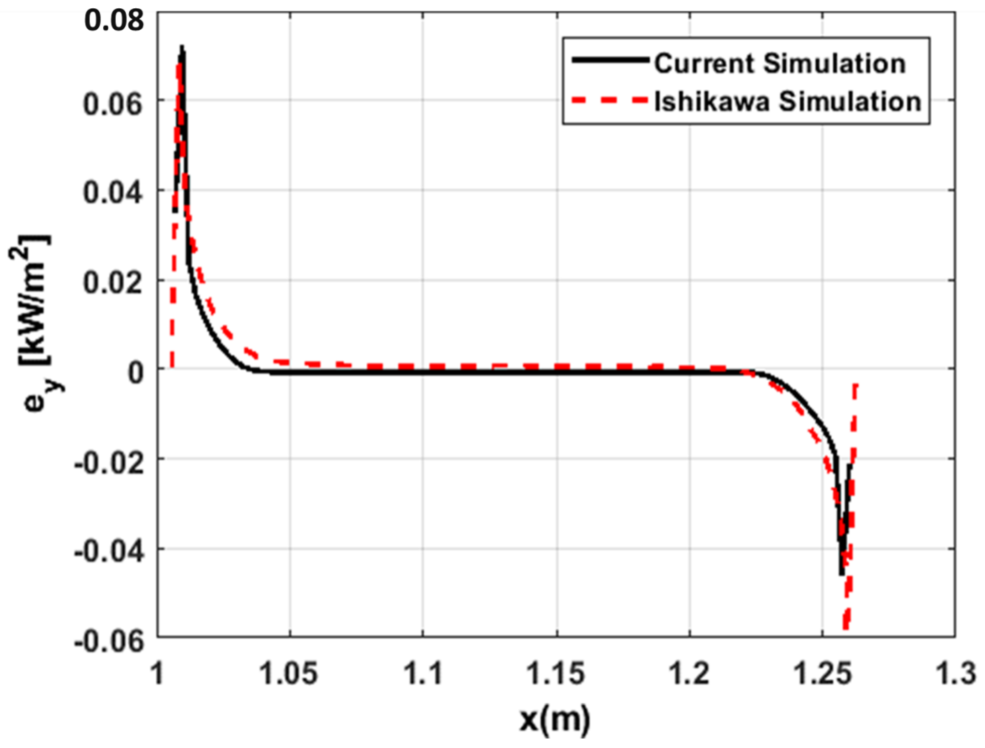
3.5. Mesh Independence and Validation Study

A mesh independence study is conducted to verify that the simulation model is independent of grid spacing and time step effects. Therefore, simulations are carried out with a homogeneous stack made of stainless steel and the profile of temperature drop produced at the middle of CHX is recorded for a time period of 1 s in each simulation. Three different spatial grids with mesh elements of 43.59 k, 9.82 k and 5.17 k cells and three different time steps namely 5 × 10⁻⁴ s, 1 × 10⁻⁴ s and 1 × 10⁻⁵ s are analyzed. The results of these simulations are shown in Figure 2a,b.

To have a convergent solution independent of spatial and temporal resolutions and to save computational time, a simulation setup with 9.82 k mesh elements and time step of 5 × 10⁻⁵ s, which is two hundredth of applied time period ($\Delta t= \tau /200$), is selected for all simulation runs. The numerically calculated phase angle between P₁ and u₁, for the selected time step, is within a maximum error of 3.06%, when compared with the ideal standing wave conditions.

The accuracy of the numerical results is further ensured by validating the simulation model with the results obtained for run 7 by Ishikawa and Mee [11]. Their simulation neglected the presence of heat exchangers and considered the stack as an isothermal plate with zero thickness. For comparison purposes, the current model is simplified to match the precise characteristics and properties of their model. The time-averaged energy flux density over the entire length of stack is evaluated and compared with the original simulated sample, as shown in Figure 3. Both results are in close agreement, which validates the accuracy of the developed simulation model.

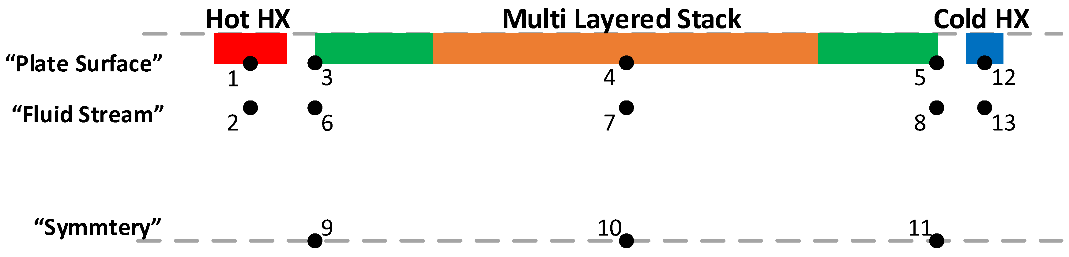
3.6. Monitor Points and Performance Scales

In order to observe the performance of the simulated zone, 13 monitor points are added, as shown in Figure 4. Nine points (3–11) are located within the stack region of simulation domain; three points located along the solid surface of plate, three in the gas stream at distance of 0.5 mm from the plate and three along the symmetry line. Span-wise location of each of these three set of points are as follows: points 3, 6 and 10 at the start (hot side), points 4, 7 and 10 at the center and points 5, 8 and 11 at the end (cold side) of stack plate. The remaining four points are located outside stack region with two points (1 and 2) in the HHX region and two points (12 and 13) in the CHX region. Points 1 and 12 are located at the center of horizontal solid surfaces of HHX and CHX, while points 2 and 13 are located in the gas stream at a distance of 0.5 mm from the solid surface. The main purpose of the points along the solid surfaces of plates is to monitor the temperatures/heat transfer rates between solid surface and surrounding fluid, while points in the fluid region can be utilized for measuring temperatures of gas stream near the solid walls and along the symmetry line of stack channel.

Performance metrics are developed for the evaluation and interpretation of obtained results in all cases. The development of the refrigeration process from onset until the steady state is an important parameter as it depicts the lowest possible temperature achievable and the rate at which a device would deliver the desired cooling. Very few numerical studies have addressed this phenomenon and most of the studies have performed simple analysis of the SWTAR performance within the stack region only. The Root Mean Square (RMS) value of temperature difference achieved at mid of CHX ($\Delta T_{CHx}$), monitor point 12, is used to gauge this parameter. $\Delta T_{CHx}$ is given by the relation:

$$\Delta T_{CHx}=T_{RMS{|}_{CHx}}-T_m$$

(30)

where $T_{RMS{|}_{CHx}}$ is the root-mean-square value of CHX temperature at monitor point 12 and its value has been averaged over the complete acoustic cycle and is given by:

$$T_{RMS{|}_{CHx}}=\sqrt{\frac{1}{\tau }{{\displaystyle \int }}_{t_0}^{t_0+\tau }{T}_{CHx}^{2}dt}$$

(31)

The Coefficient of Performance (COP) and time-averaged total energy flux in the y-direction across the stack ($\langle {\dot{E}}_y\rangle {}_t$) are also calculated, using Equations (13) and (16), respectively, for each case.

The second major performance metric employs the distribution of time-averaged values at various segments of the domain, where the averaging is performed over a complete cycle for every parameter under investigation. Time-averaged temperature distribution over the stack plate, $\langle T_{stack}\rangle {}_t$, is utilized to evaluate the axial distribution of temperature for various material and length combination of stacks. Time-averaged energy flux density distribution across the stack-fluid interface, ${\langle \dot{e}\rangle }_t$ is a very useful parameter and it has been evaluated in the majority of reported SWTAR numerical studies [11,14,21,23]. Since the current work considered stacks of non-zero thickness, both the horizontal and vertical surfaces will experience the energy flux. Thus, the quantity $\langle {\dot{e}}_y\rangle {}_t$ is monitored along the stack surfaces to calculate the energy flux density along y-direction.

Temperature difference between the solid surface of stack and gas stream is also an important parameter as it dictates the heat transfer mechanism between solid and gas and can be defined as:

$$\Delta T_{1{|}_{g,s}}=T{|}_{y=y_0}-T{|}_{y=y_0-0.2{\delta }_k}$$

(32)

For an effective evaluation of heat transfer process, the profile of $\Delta T_{1{|}_{g,s}}$ parameter over a complete period of acoustic cycle is monitored at two different locations, i.e., stack cold end (x = 1.26 m) and center of CHX (x = 1.2625 m). The monitor points at each location are 5 and 8 and 12 and 13, respectively.

The time required to reach steady state for each simulation is estimated to be at least ≥ 300 s (5 min) which corresponds to computational time of 207.82 days on Intel Xeon E52650, 2.60 GHz CPUs. The numerical simulation requires a very long computational time to reach steady state at CHX. Therefore, all the measurements are recorded for a physical time of at least 30 s for all test cases, while simulation time is extended to 90 s for the length variation cases and performance evaluation is carried out at these time scales. Steady state values of $\Delta T_{CHx}$ for each case are estimated using exponential extrapolation. The exponential function utilized to reproduce the results is given by the following equation:

$$\Delta T=a+b.\left(1-e^{c.t}\right)+d.\left(1-e^{f.t}\right)$$

(33)

where a, b, c, d and f are fitting constant and t is the global time for the simulation. In the first stage, to validate the accuracy of the exponential extrapolation, an exponential fitting is performed on graphical data provided in the published work of Rahpiema and Ebrahimi [26]. For the said purpose, fitting is conducted on the time history plot of $\Delta T_{CHx}$ produced for 0.1 mm thick stainless steel stack. The extrapolated function estimated the curve with a Root-Mean-Square Error (RMSE) of 0.48%. Since the current model simulates the exact domain used by Rahpiema and Ebrahimi [26] for a homogeneous stack case, the same exponential function is further applied to extrapolate the results for all cases of the current work.

4. Results and Discussion

Application of an oscillatory boundary condition at the right side of the truncated domain resulted in a sinusoidal oscillating pressure ($P_1$) with an amplitude of 113.6 Pa while the amplitude of oscillating velocity ($u_1$) is around 7.955 m/s. The development of pressure and velocity profiles at the start of the simulation are shown in Figure 5. In Figure 5b, it is apparent that the velocity profile shows a transient behavior at the first few cycles before it becomes periodic with a mean velocity of approximately 0.111 m/s. These conditions of pressure and velocity at inlet boundary will result in a constant acoustic power inside the domain as the major geometric and operating parameters, i.e., L_s, y₀, th, stack center position (x_n), P_m and DR, are constant for all cases. The time-averaged value of the acoustic power for one complete cycle is calculated as, ${\langle \dot{W}\rangle }_t$ = 263 W.

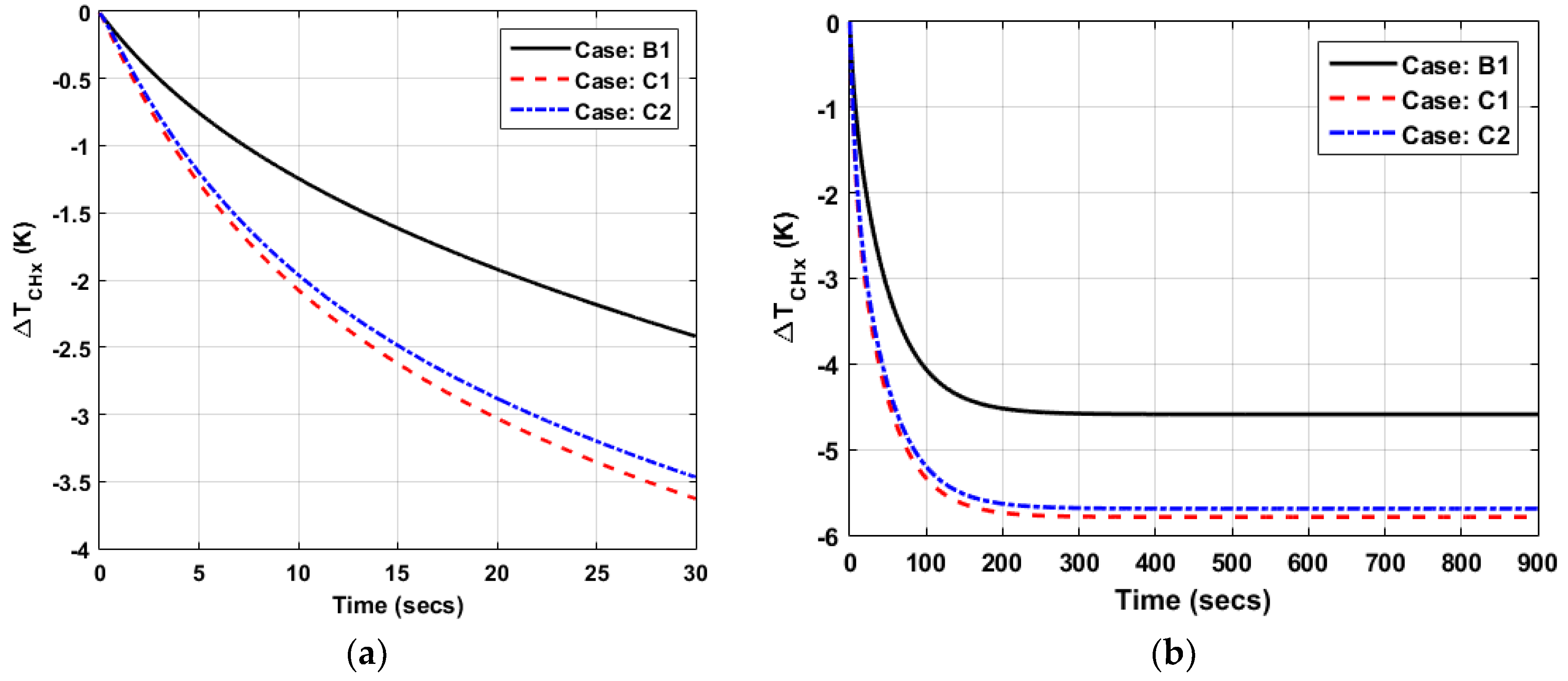
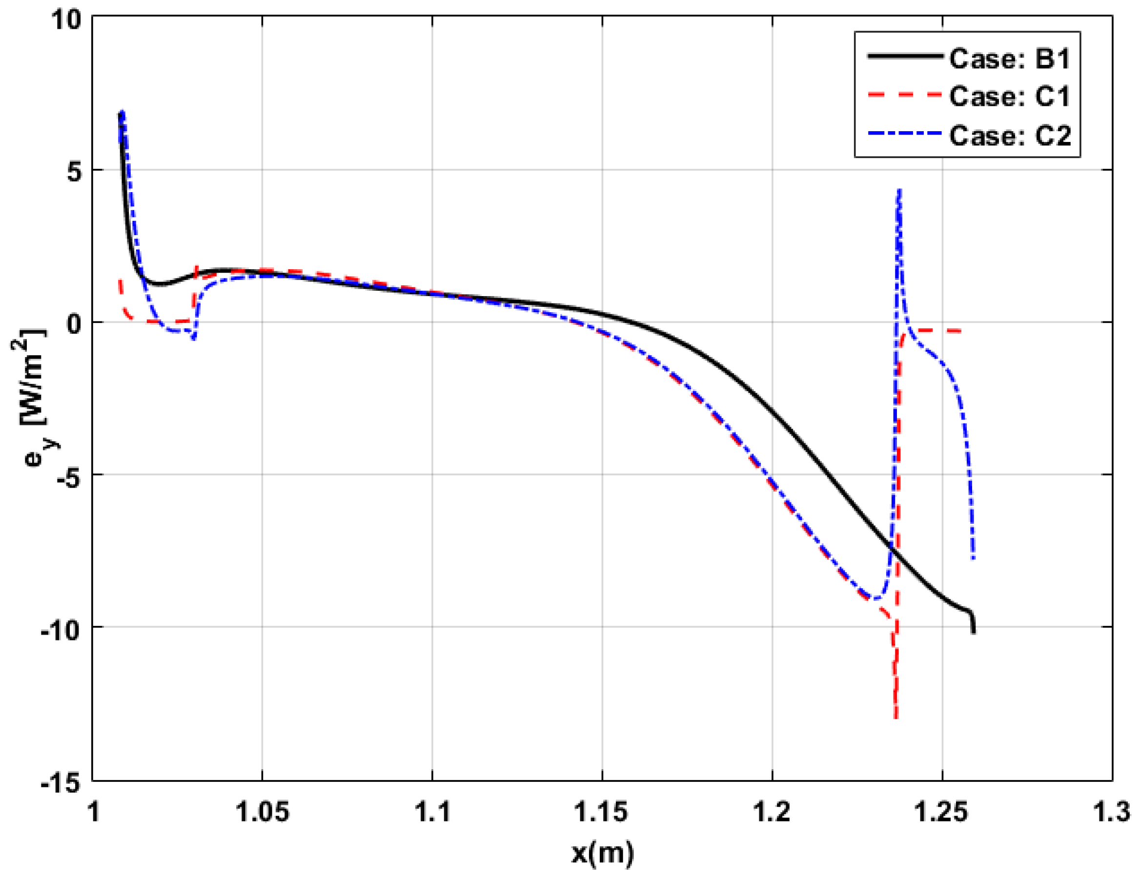
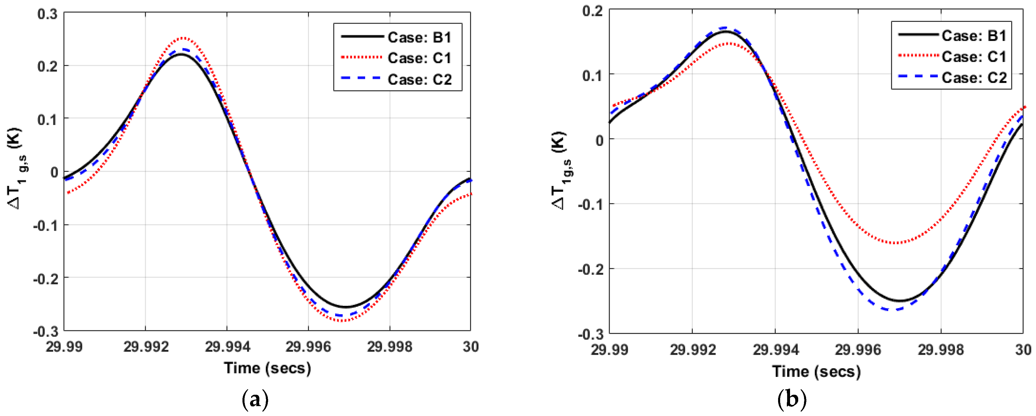
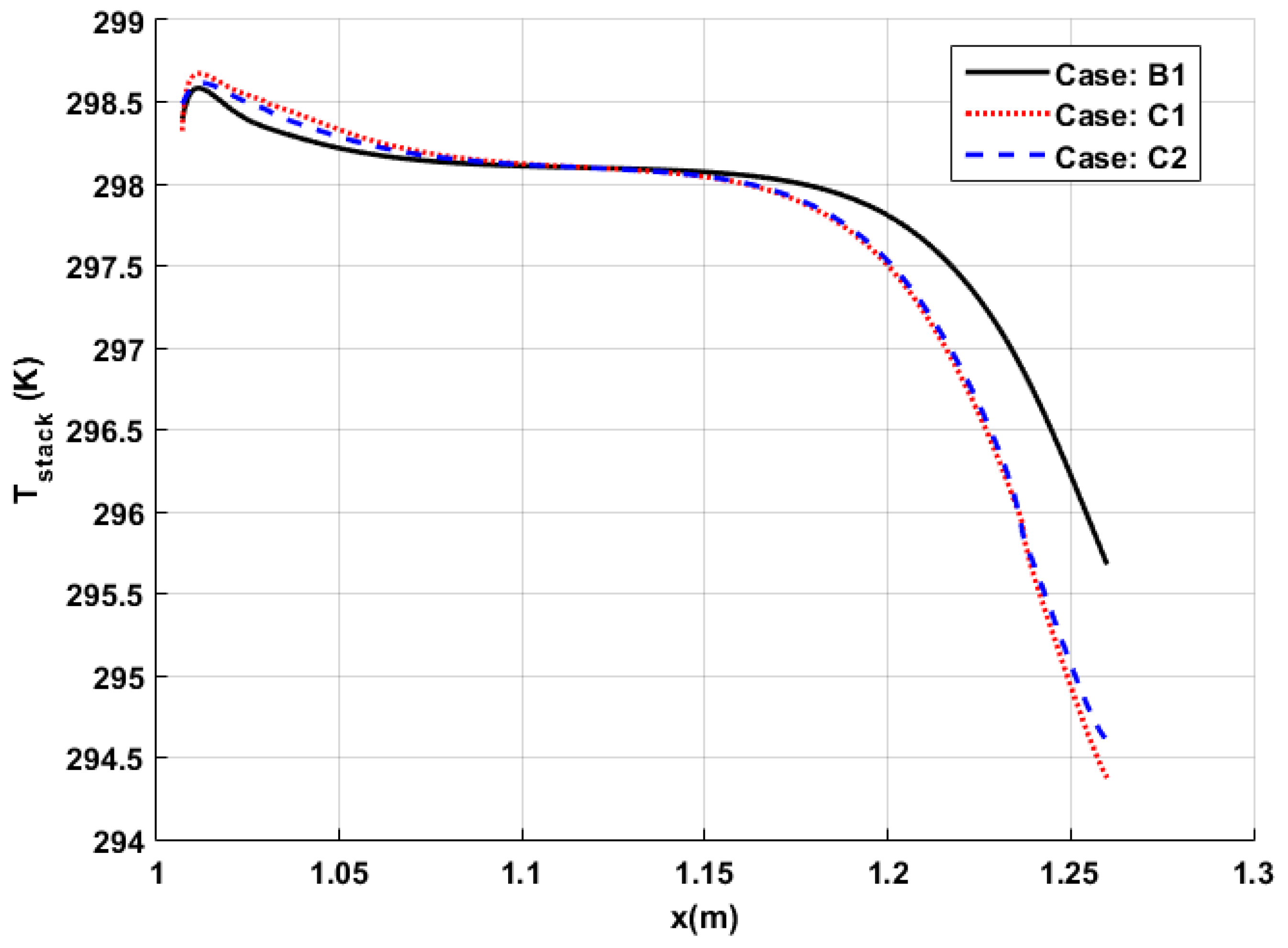
4.1. Effect of Different Material Combinations of Multi-Layered Stack

This section presents the evaluation of performance of SWTAR for various material combinations of multi-layered stack.

Table 4. Performance results for Celcor based material combination of stack.

Case	$\mathbf{\Delta }{\mathit{T}}_{\mathit{C}\mathit{H}\mathit{x}}(\mathbf{K})$ (Steady State)	$\langle {\dot{\mathit{E}}}_{\mathit{y}}\rangle {}_{\mathit{t}}(\mathbf{W})$	COP
B1	4.59	79.26	0.254
C1	5.79	75.64	0.261
C2	5.69	76.89	0.255

tabulates the performance results, along with the extrapolated steady state values, obtained for three cases having Celcor as base material. The results of two material combinations having Celcor as a base material, i.e., C1 and C2, are compared with those obtained for homogenous stack made of Celcor (B1). It is worth mentioning that the length of each material layer (M_R or M_L) stacked at either side, in both C1 and C2, is 23 mm (equivalent to 1PD) and the length of the base material is 207 mm.

The results obtained clearly demonstrate that the presence of different material layers in the stack have a significant effect on the refrigeration performance. Based on the estimated steady-state values for temperature drop, $\Delta T_{CHx}$, multi-layered stacks C1 and C2 produced approximately 26.14% and 23.96% higher refrigeration temperatures than homogenous stack B1. The transient profiles of refrigeration process for cases B1, C1 and C2 are depicted in Figure 6a while the extended profiles of $\Delta T_{CHx}$ up to the steady-state are shown in Figure 6b. The cooling curves in Figure 6b are extrapolated using the function described in Equation (33) while the values of the fitting constants are provided in

Table 5. Fitting constants for exponential extrapolation of various material combinations of multi layered stacks.

Case/Fitting Constant	a	b	c	d	e
B1	−0.01396	−0.5908	−0.1857	−3.985	−0.02029
B2	−0.006375	−0.7127	−0.1563	−4.853	−0.01884
C1	0.005943	−1.628	−0.1462	−4.168	−0.02222
C2	0.03373	−1.525	−0.1499	−4.201	−0.02147
C3	0.008403	−1.487	−0.147	−4.876	−0.02347
C4	0.03299	−1.411	−0.1473	−4.947	−0.02177

. The extrapolated steady-state values using the 30 s data are compared with those obtained after 90 s for selected cases, revealing a very good agreement and yielding the 30 s data adequate to perform further analysis of the results. It is evident from the current simulations that the time required by the cooling process to reach steady-state is at least 300 s.

Ideally, the stack acts as a perfect thermal barrier between hot and cold sides to allow maximum heat transfer to take place at heat exchangers [36]. Energy flux density is a useful parameter in the prediction of energy transfer. The parameter $\langle {\dot{E}}_y\rangle {}_t$ indicates the time-averaged energy absorbed by stack during a complete cycle. Higher values of $\langle {\dot{E}}_y\rangle {}_t$ are not appreciated as it degrades the performance of CHX by adding undesirable thermal load [1]. Hence, the larger the value of $\langle {\dot{E}}_y\rangle {}_t$, the lower the performance of stack, and from the results given in Table 4 it can be seen that case C1 has the lowest value followed by C2, and then B1. Thus, $\langle {\dot{E}}_y\rangle {}_t$, consumed by the stacks of C1 and C2, are less than stack of B1 by an amount of 4.55% and 2.97%, respectively.

For a constant acoustic power, ${\langle \dot{W}\rangle }_t$ the COP values indicate the amount of heat transfer taking place at CHX. Higher the heat transfer at CHX, i.e., $\langle {\dot{Q}}_{CHx}\rangle {}_t$, higher is the COP of the device and better is the performance of SWTAR. The COP values obtained are tabulated in Table 4 illustrating that C1 is the best combination. The device COP is enhanced by an amount of 5.12% and 0.39% for cases C1 and C2, respectively, when compared with case B1.

The optimum performance is achieved when material of the stack is selected with low thermal conductivity and high specific heat capacity so that it can have minimal axial conduction and high heat retention [36]. Among the three materials considered in the above discussion, RVC has the lowest thermal conductivity, followed by Celcor and Aluminum (Al), while the specific heat capacity of RVC is highest followed by Celcor and Al. Therefore, the combination C1 has the best properties among all the three cases, resulting in the highest value of temperature drop ($\Delta T_{CHx}$), lowest value of $\langle {\dot{E}}_y\rangle {}_t$ consumed and highest COP value.

The effect of having different material layers at either side of the stack can be best visualized and evaluated by observing the distribution of energy flux density over the whole length of stack. Time-averaged energy flux density $\langle {\dot{e}}_y\rangle {}_t$ is positive for heat leaving the fluid and entering the plate surface and negative for heat leaving the plate surface. Figure 7 shows the distribution of $\langle {\dot{e}}_y\rangle {}_t$ for the three Celcor based material combinations, i.e., B1, C1 and C2. For the homogeneous Celcor stack (B1), a maximum negative $\langle {\dot{e}}_y\rangle {}_t$ value is observed at the cold end of the stack (x = 1.260 m), resulting in the transfer of heat from the solid plate to the fluid at this end. This negative $\langle {\dot{e}}_y\rangle {}_t$ amplitude shifts towards left side of the stack by an amount equal to 1PD for cases C1 and C2 due to the presence of different material at the end. The span of the negative $\langle {\dot{e}}_y\rangle {}_t$ values is quite large for all the cases accounting to almost 60% of stack length (x = 1.160 m or 0.6 L_s). Despite the shifting of the negative $\langle {\dot{e}}_y\rangle {}_t$amplitude towards left for multi-layered stacks, the change in the direction of $\langle {\dot{e}}_y\rangle {}_t$ value from negative to positive occurs at almost the same location along the stack for all three cases. The transition location is around x = 1.105 m, which is approximately 0.38 L_s illustrating asymmetric distribution of energy flux along the plate. This type of asymmetry is, in fact, present in every simulation involving thermoacoustic couple due to the variable velocity amplitude along the stack length, but it is not captured by models having stacks with zero thickness [11,14,20]. The time-averaged energy flux at transition point is positive in the transient response and it would approach zero value as the simulation approaches steady state.

For the case of C1, the maximum negative $\langle {\dot{e}}_y\rangle {}_t$ amplitude is still observed at the right end (cold side) of middle Celcor layer but it drops quickly in the RVC segment. Thus, negligible heat transfer take place along the RVC segment resulting in formation of an insulation zone at the end of the stack. As a result, during the expansion phase of acoustic wave, the gas particle travels towards the right side along the cold end, absorbs minimal heat from the stack and maintains its lower temperature. Upon reaching the CHX, there will be a maximum temperature difference available between the solid and gas resulting in a higher heat transfer. This is also true for the compressive phase, but in this phase, the gas particle will travel to the left and it will enter the stack after leaving the CHX. The presence of insulation zone will allow the gas particle to move towards the hotter side with minimal heat transfer to the stack while maintaining its temperature, thus reducing the unwanted heat transfer. The presence of an insulation zone caused a decrease in the overall energy flux which allows more heat transfer to take place at CHX location, thus enhancing the performance of device.

For the combination C2, where a slightly conductive Al layer is placed at stack ends, another negative $\langle {\dot{e}}_y\rangle {}_t$ peak is observed at end of Al layer (cold end) having a lower amplitude compared to the end of Celcor layer. Hence, a finite amount of heat transfer takes place between the fluid and solid inside the stack in this region. It will cause a slight increase in the temperature of gas particle compared to RVC case. Therefore, a lower temperature difference is maintained between the fluid and solid at CHX location and it will lower the refrigeration performance of device compared to performance of combination C1. The interface between two materials in the cases C1 and C2 results in the formation of an extra sharp peak due to numerical inconsistencies.

Temperature difference between the solid surface of stack and gas stream is also an important parameter as it describes the heat transfer mechanism between solid and gas particles. Figure 8a,b compares the profiles of $\Delta T_{1{|}_{g,s}}$, for one complete cycle, for cases B1, C1 and C2 at two different locations, i.e., at mid of CHX and at cold end of stack. The higher the amplitude of $\Delta T_{1{|}_{g,s}}$, higher is the heat transfer between solid and gas at that location. The observations of Figure 8a inferred that, at the mid of CHX, the maximum value of $\Delta T_{1{|}_{g,s}}$ is recorded for combination C1 and the minimum for B1. Therefore, C1 has the highest heat transfer rate resulting in lowest temperature value. Furthermore, for an efficient refrigeration, stack should have minimal involvement in the heat transfer process, i.e., its temperature should remain close to the temperature of the nearest gas particles. Therefore, a complete reverse trend is observed at cold end of stack, as shown in Figure 8b. Thus, the combination C1 has the lowest values of $\Delta T_{1{|}_{g,s}}$ at cold end of the stack. These findings further confirm the explanation provided for energy flux distribution at stack ends for multi-layered stack. The negative half of the cycle in Figure 8b is associated with the unwanted heat being transported to gas particles and then to the CHX. It is evident that the presence of a conductive layer at the stack ends in combination C2 results in the highest value of unwanted heat flux. Thus, combination C2, despite having comparable performance in terms of $\Delta T_{CHx}$, has the highest irreversible losses. The graphs for B1 and C2 in Figure 8b are asymmetric with respect to $\Delta T_{1{|}_{g,s}}$ amplitudes (higher for the negative half), indicating a net loss of heat to the stack during the compressive phase. Symmetric trend is observed for the case C1, confirming it to be the best combination in terms of unwanted heat loss.

Time-averaged axial temperature distribution over stack plate surface for cases B1, C1 and C2 is shown in Figure 9. It is illustrated that the temperature of the plate is nearly constant around T_m value in the region of 0.3 L_s to 0.55 L_s and it starts to decrease along the plate length where the energy flux density is negative. Although the temperature of the HHX is kept fixed at T_m = 298 K, a high temperature region is observed near the hot side of the stack due to presence of positive energy flux in this region, as previously illustrated in Figure 7. Since the cooling process did not reach its steady state, the temperature distribution along the plate is varying and uniform temperature gradient will develop across the stack plate once the steady state has been reached.

Performance results obtained for Kapton-based material combinations, i.e., B2, C3 and C4, are given in

Table 6. Performance results for Kapton-based material combinations of stack.

Case	$\mathbf{\Delta }{\mathit{T}}_{\mathit{C}\mathit{H}\mathit{x}}\left(\mathbf{K}\right)$ (Steady State)	$\langle {\dot{\mathit{E}}}_{\mathit{y}}\rangle {}_{\mathit{t}}(\mathbf{W})$	COP
B2	5.57	77.23	0.247
C2	6.36	74.07	0.268
C3	6.33	75.37	0.261

. The steady state values achieved for$\Delta T_{CHx}$ are extrapolated using exponential function given by Equation (33) and fitting constants utilized are given in Table 5. The pattern of the results obtained is similar to those obtained for the Celcor based combinations. The combination C3 produced the best results. Based on the steady state values, both combinations of multi-layered stacks, i.e., C3 and C4 reached the refrigeration temperatures that are approximately 14.18% and 13.64% lower than homogenous Kapton stack B2. Similarly, the values of $\langle {\dot{E}}_y\rangle {}_t$ absorbed by C3 and C4 are lower than B2 by an amount of 4.09% and 2.41%, respectively. Device COP is increased by 8.50% and 5.67% for cases C3 and C4, respectively.

A comparison of $\Delta T_{1{|}_{g,s}}$ for Kapton-based combinations, at two different locations, i.e., mid of CHX and at stack cold end, provided results similar to those illustrated in Figure 8. The combination C3, having RVC at the ends, has the maximum temperature difference and subsequently highest heat transfer rate resulting in maximum refrigeration performance. Combination C4 with Al as side layers resulted in the highest losses inside the stack during the compressive phase. Thus, the performance results displayed in Table 6 for the cases B2, C3 and C4 are consistent and similar to those discussed earlier for Celcor based combinations.

The overall performance of Kapton-based stacks is slightly better than its Celcor-based counterpart. This can be attributed to the fact that Kapton has lower thermal conductivity and higher specific heat capacity values compared to Celcor.

For an effective assessment of the performance of stack with different material combinations, performance parameters, such as $\langle {\dot{E}}_y\rangle {}_t$ and COP, are calculated for the same $\Delta T_{CHx}$ produced in each case. For this purpose, the value of $\Delta T_{CHx}$ obtained for the case B1 after 30 s, i.e., 2.42 K, is selected as a reference. The same value of $\Delta T_{CHx}$ is achieved at different times for all other cases, i.e., 12.9, 14.3, 23.2, 12.0 and 13.3 s for C1, C2, B2, C3 and C4, respectively. The obtained performance parameters are then normalized with respect to the respective values obtained for case B1 and are depicted in Figure 10 in the form of a bar graph.

Results displayed in Figure 10, in terms of $\langle {\dot{E}}_y\rangle {}_t$, show that, for a given cooling load, all stack combinations consumed less energy flux when compared with the value absorbed by homogeneous Celcor stack (case B1). The $\langle {\dot{E}}_y\rangle {}_t$ values for combinations C1 and C2 are less than their homogeneous counterpart B1 by 1.64% and 0.39%, respectively. Combination C1 has the best performance among Celcor based stacks, followed by C2. Similarly, for Kapton-based stacks, combination C3 produced the best results followed by C4 and then B2. The values of $\langle {\dot{E}}_y\rangle {}_t$ obtained for B2, C3 and C4 are less than $\langle {\dot{E}}_y\rangle {}_t$, the value of the case B1, by 1.54%, 2.95% and 2.13%, respectively.

For a given$\Delta T_{CHx}$, combinations C1 and C3 have the highest COP values among Celcor and Kapton-based stacks. The COP value for C1 is 12.81% higher than COP value of B1 and this percentage increases to 17.18% for C3. Performance improvement in terms of COP, taking B1 as the base case, for cases C2, B2 and C4 are 8.08%, 3.35% and 13.63%, respectively.

To conclude, current numerical simulations suggested that the presence of several layers of different materials inside the stack improve the SWTAR performance. Multi-layered stacks produce lower refrigeration temperatures, consume less energy and have higher COP value than their homogeneous counterparts. Among all the material combinations of multi-layered stack investigated, stacks having a material with a lower thermal conductivity at ends, i.e., RVC, produced the best performance. Material combinations having conductive layer at the stack ends, i.e., Al, have comparable performance in terms of $\Delta T_{CHx}$ but have the highest losses in terms of undesirable thermal load, even higher than their homogeneous counterparts.

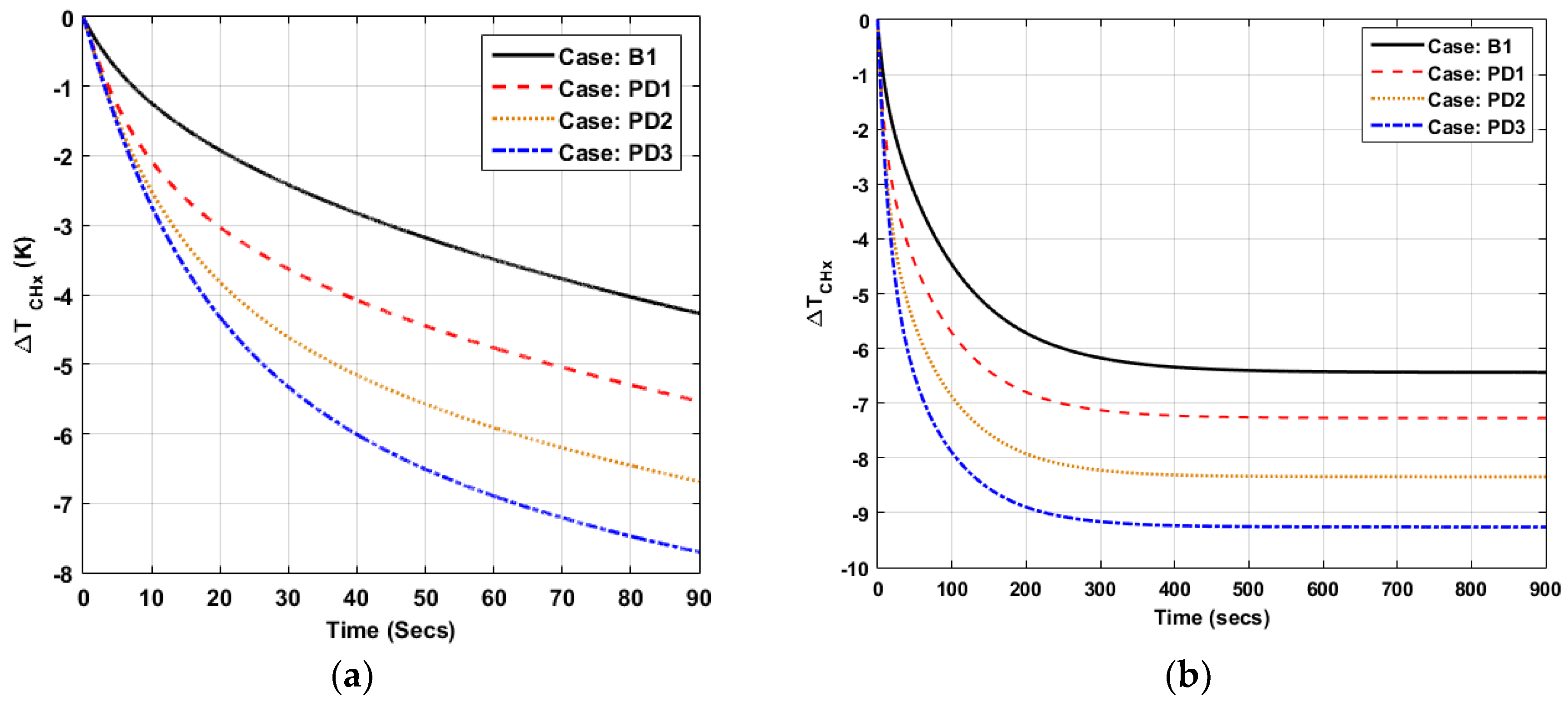
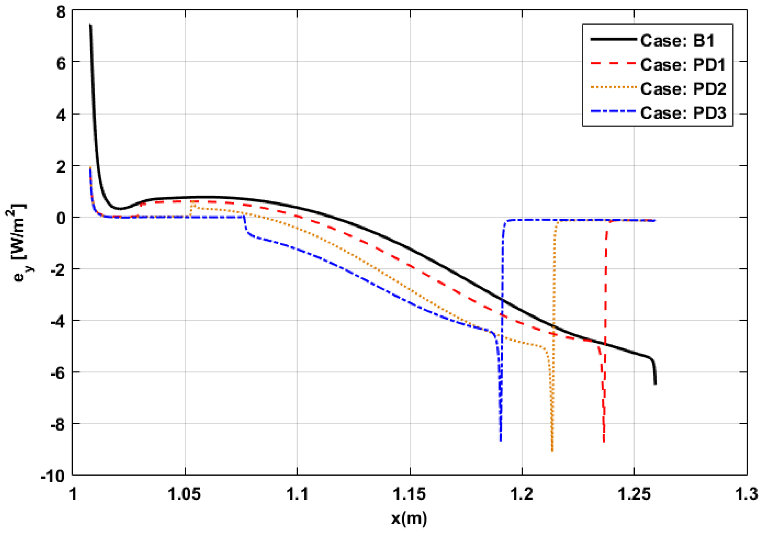
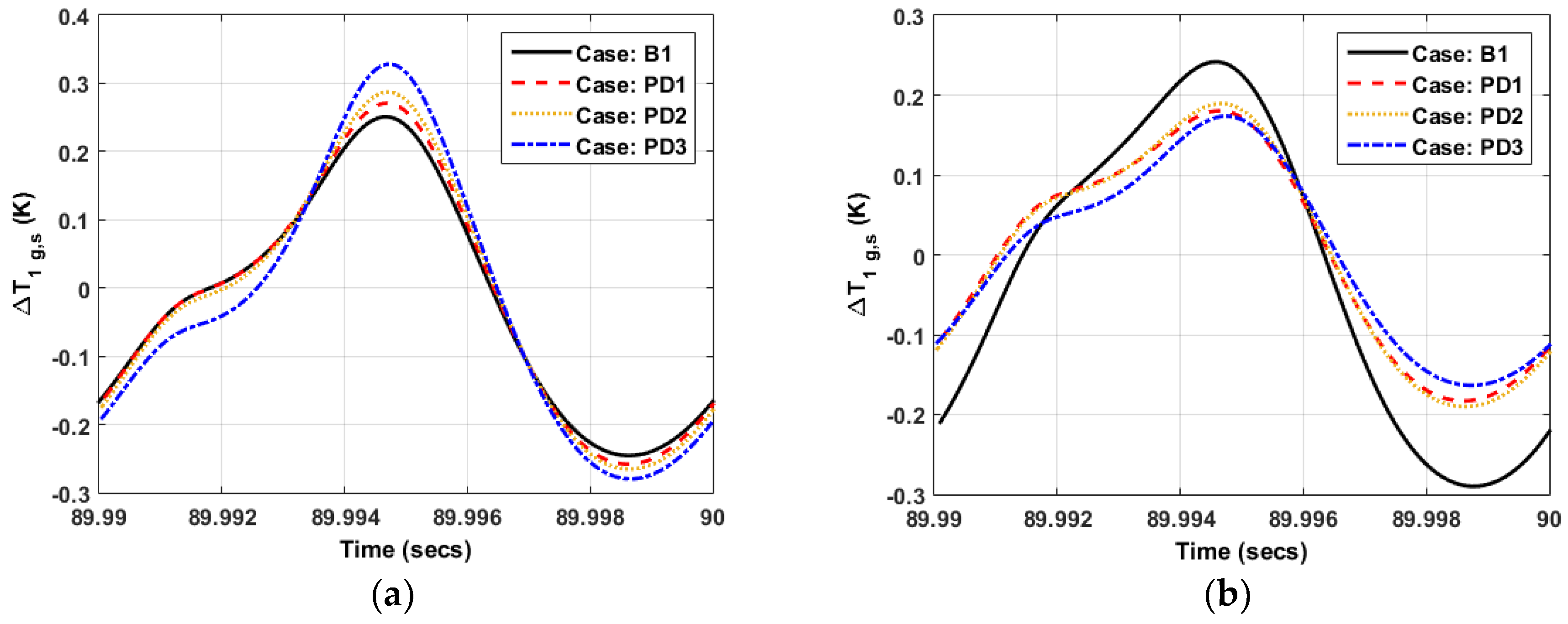
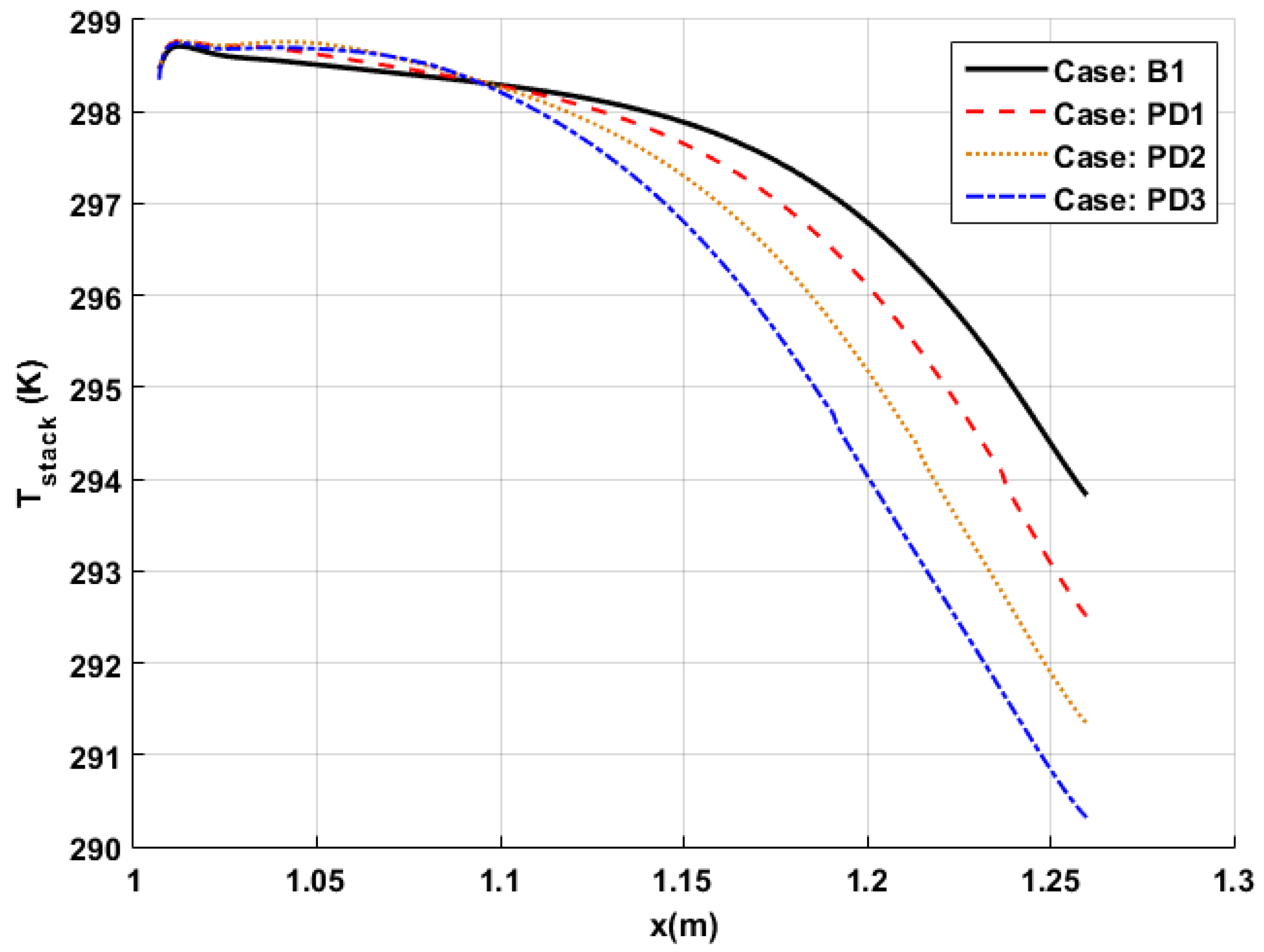
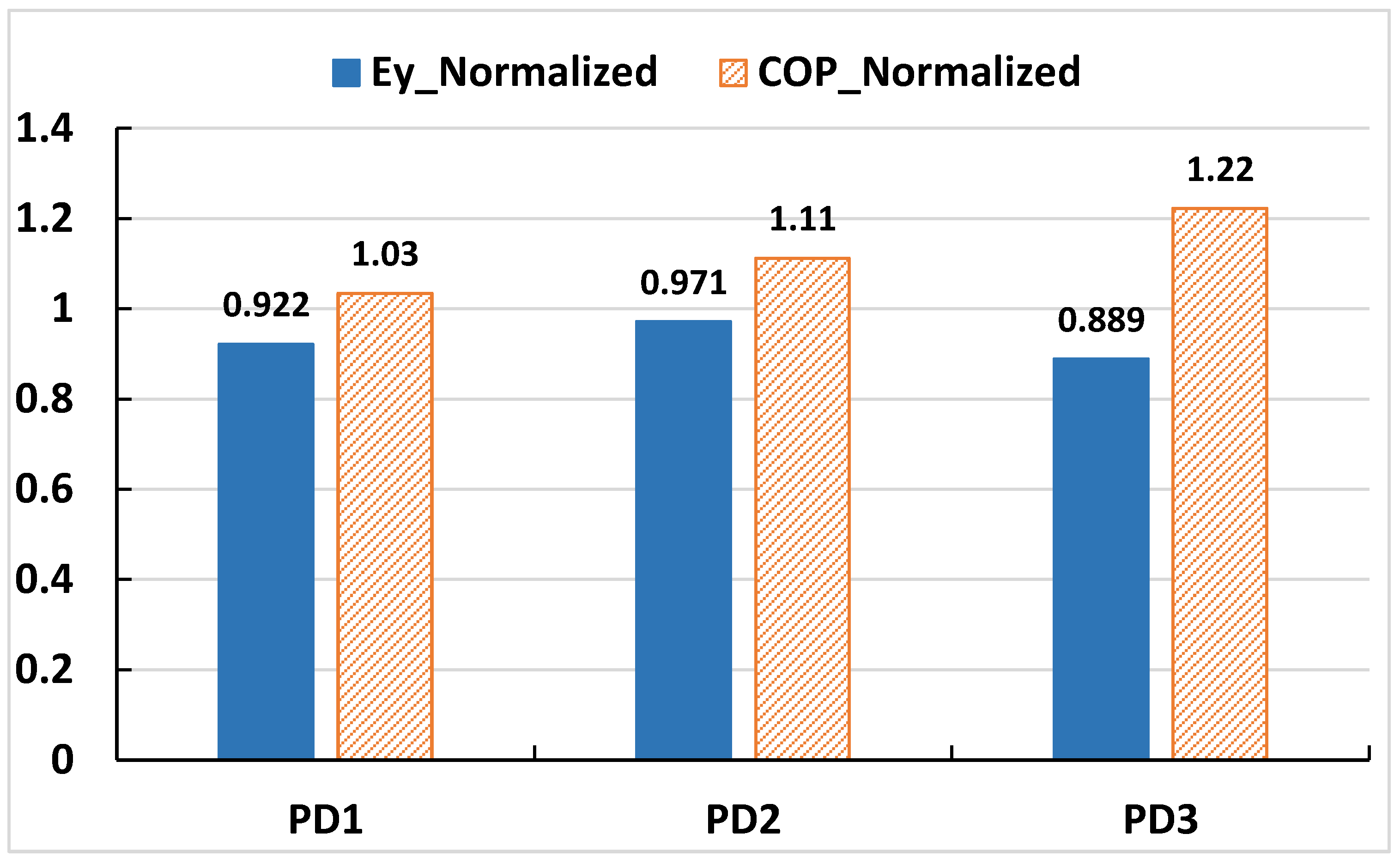
4.2. Effect of Variation in Length of Layers of Multi-Layered Stack

RVC based multi-layered stacks produced the best performance among all material combinations evaluated. Therefore, multi-layered stack combination made of Celcor as a base and RVC at both ends (RVC, Cel, RVC) is selected to further evaluate the variation in length of individual segments of the stack. The simulations of the length variation cases are carried out for an extended duration of 90 s before approximating the steady state response using extrapolation. The data points are utilized by a curve fitting tool to predict the transient behavior and estimate the time constants. The overall length of the stack (L_s) is kept constant, i.e., 253 mm and the length of individual layers is varied as a function of PD which is equivalent to 23 mm for the current setup. Based on the naming conventions defined in Table 1, the following length cases are investigated: B1 or (PD0), PD1 or (C1), PD2 and PD3.

Performance results obtained for all the length cases are summarized in

Table 7. Performance results for different length combinations of stack.

Case	$\mathbf{\Delta }{\mathit{T}}_{\mathit{C}\mathit{H}\mathit{x}}\left(\mathbf{K}\right)$ (Steady State)	$\langle {\dot{\mathit{E}}}_{\mathit{y}}\rangle {}_{\mathit{t}}(\mathbf{W})$	COP
B1	6.44	80.61	0.252
PD1	7.27	71.62	0.265
PD2	8.35	73.08	0.275
PD3	9.26	65.13	0.284

. It can easily be seen that as the length of side stack layer is increased gradually from 0 to 3 PD, the value of $\Delta T_{CHx}$ increases. Case B1 has the smallest temperature drop with a value of 6.44 K and the largest drop is observed for PD3 which is 9.26 K.

The temporal development of $\Delta T_{CHx}$ is shown in Figure 11a while the steady state response is shown in Figure 11b. Based on the steady state results, depicted in Table 7, replacement of Celcor material with RVC layer of three PD length at stack ends resulted in a net increase of 43.79% in the refrigeration performance. The plots of $\Delta T_{CHx}$ are extrapolated using the exponential function given by Equation (33) and fitting constants utilized in generation of these plots are given in

Table 8. Fitting constants for exponential extrapolation of various length combinations of multi-layered stacks.

Case/Fitting Constant	a	b	c	d	E
B1	−0.06661	−5.387	−0.01007	−0.9842	−0.1099
PD1	−0.03323	−5.117	−0.01192	−2.121	−0.1170
PD2	0.01577	−5.109	−0.01248	−3.252	−0.08966
PD3	0.03041	−5.067	−0.01317	−4.224	−0.07003

.

The COP value also increases with an increase in the length of side-stacked layers. In other words, as the length of RVC portion is increased, the device performance is enhanced by allowing higher heat transfers to take place at CHX location. Performance enhancement of device in terms of COP is 12.70% as RVC length is increased from 0 to 3 PD. In terms of $\langle {\dot{E}}_y\rangle {}_t$, homogeneous Celcor stack (B1) absorbed the highest energy flux thus resulting in the lowest refrigeration performance. The value of $\langle {\dot{E}}_y\rangle {}_t$ is decreased as the length of side stacked is decreased. Length case PD2 showed different trend compared to results of $\Delta T_{CHx}$ and COP. It is observed that it has the highest value among the three selected length combinations of multi-layered stacks. Based on the results of all three parameters, combinations PD3 have better overall parameters among all the selected length cases.

Time-averaged energy flux density, $\langle {\dot{e}}_y\rangle {}_t$, distribution over the stack plate for all length cases are shown in Figure 12. The negative $\langle {\dot{e}}_y\rangle {}_t$ amplitudes observed at the right end of Celcor layer vanishes and $\langle {\dot{e}}_y\rangle {}_t$ becomes almost negligible in the entire RVC part of the stack for all length cases. It results in the formation of insulation zone at the stack end. Thus, larger the length of RVC layer, the larger the insulation zone created inside the stack and the higher the performance of SWTAR in terms of $\Delta T_{CHx}$ and COP. The enhanced device performance is once again attributed to the capacity of stack to have minimal heat transfer with the fluid allowing the fluid parcel to absorb more heat from CHX during the expansion phase. The negative $\langle {\dot{e}}_y\rangle {}_t$ peak observed for PD2 is once again higher than peaks of PD1 and PD3 thus confirming the results tabulated in Table 7.

The curves in Figure 13 show the profile of $\Delta T_{1{|}_{g,s}}$ for all four cases with length variation. Results are plotted for one acoustical cycle at two locations, i.e., mid of CHX and cold end of stack. At the mid of CHX (Figure 13a) maximum $\Delta T_{1{|}_{g,s}}$ is observed for case PD3 having the largest length of RVC placed at both sides of the stack. The amplitude of $\Delta T_{1{|}_{g,s}}$ decreases as these lengths are reduced and a minimum value is obtained for B1. These results reiterate the outcomes of stack performance parameters, given in Table 7, as the highest heat transfer will take place for the case having maximum$\Delta T_{1{|}_{g,s}}$ at CHX. The peculiar behavior of PD2 stack observed in the results of energy flux ($\langle {\dot{E}}_y\rangle {}_t$) is also observed in the profiles of $\Delta T_{1{|}_{g,s}}$ at the cold end of stack, shown in the Figure 13b. The highest value of $\Delta T_{1{|}_{g,s}}$ is observed for case B1, followed by PD2, PD1 and PD3 in a decreasing fashion.

Axial distribution of time-averaged temperature along the stack length is depicted in Figure 14. For all length cases, the hot end of the stack has attained a constant temperature around 298.7 K, slightly higher than T_m, and this temperature is maintained for the entire length of RVC layer. After that, it decreases gradually until the cold end of stack. Temperature variation on the cold side of the stack is linear in the entire region of RVC layer, thus highlighting the saturation of temperature profile within that portion. The temperature profile at the stack ends highlights the effect of having low thermal conductivity material.

For an effective performance comparison of all length combinations, the results of $\langle {\dot{E}}_y\rangle {}_t$ and COP are evaluated for the same $\Delta T_{CHx}$ achieved by each case. The value of 4.27 K achieved for case B1 in 90 s is selected as a reference and the performances of all other cases are evaluated for this cooling load. The results for $\langle {\dot{E}}_y\rangle {}_t$ and COP are normalized with respect to the values obtained for case B1 and presented in Figure 15. The obtained results are similar to those tabulated in Table 7. It can be observed that for an equal cooling load, all the length cases consumed lower $\langle {\dot{E}}_y\rangle {}_t$ and have higher COP values than homogenous stack B1. Energy flux values of PD1, PD2 and PD3 are less than B1 by 7.80%, 2.86% and 11.14%, respectively. The COP of SWTAR increases as the length of RVC layer inside the stack is increased. When compared with results of B1, the improvement in COP for PD1, PD2 and PD3 are 3.47%, 11.19% and 22.21%, respectively.

To conclude, the results indicate that the addition of a layer of insulative material at stack ends, even for lengths as small as one particle displacement length, has a positive effect on the refrigeration performance of SWTAR. However, the maximum benefit could be obtained if the lengths of the end layers are kept to around one and three PD as the length combination PD2 consumed much higher energy flux for the same amount of cooling.

5. Conclusions

The effect of the multi-layered stack on the refrigeration performance of a SWTAR has been studied numerically using a detailed CFD approach. Two different aspects of multi-layered stack, namely, different material combinations and different layer lengths, are investigated in terms of $\Delta T_{CHx}$, $\langle {\dot{E}}_y\rangle {}_t$ and COP. Eight cases, including four different material combinations and four length ratios, are analyzed.

It can be observed that the using a stack made of layers of different materials may improve the SWTAR performance. Multi-layered stacks produce lower refrigeration temperatures, consume less energy and have higher COP value than their homogeneous counterparts. Among all the material combinations of multi-layered stack investigated, stacks having a material layer with lower thermal conductivity at the ends, i.e., RVC, produced the best performance.

The values of $\Delta T_{CHx}$, $\langle {\dot{E}}_y\rangle {}_t$ and COP obtained using Celcor based RVC combination C1 are 5.79 K, 75.64 W and 0.261, respectively. For Kapton-based RVC combination C3, these values are 6.36 K, 74.07 W and 0.268, respectively. The performances of C1 and C3, when compared with their homogeneous counterparts B1 and B2, show that $\Delta T_{CHx}$ values increased by 26.14% and 14.18%, $\langle {\dot{E}}_y\rangle {}_t$ consumption was reduced by 4.55% and 4.09% and COP of SWTAR was enhanced by 5.12% and 8.50%, respectively.

For the case of varying the lengths of individual stacked layers, it can be concluded that the addition of a layer of insulative material at the stack ends, even for lengths as small as one particle displacement length, has a positive effect on the refrigeration performance of SWTAR. However, the maximum benefit is observed when the lengths of end layers are kept around one or three PD, while the length combination PD2 consumes higher energy flux for the same amount of cooling.

Moreover, for a constant overall length, an increase in the length of side stacked material layer results in an increase in values of both $\Delta T_{CHx}$ and COP. The maximum temperature drop, $\Delta T_{CHx}$, of 9.26 K has been achieved for case PD3 with an improvement of 43.79% when compared to the value attained for B1. Similarly, COP of SWTAR for PD3 is 0.284, which is 12.70% higher than the value of stack B1.

For the visualization and explanation of the above results, the distribution of time-averaged energy flux density over stack plate ($\langle {\dot{e}}_y\rangle {}_t$) and the difference in oscillating temperature of solid surfaces and gas stream ($\Delta T_{1{|}_{g,s}}$) is also illustrated. The distribution of $\langle {\dot{e}}_y\rangle {}_t$ showed that cases having the largest negative amplitudes consumed highest energy flux while $\Delta T_{1{|}_{g,s}}$ profiles showed that cases having the highest $\Delta T_{1{|}_{g,s}}$ values at CHX location, have the maximum performance in terms of $\Delta T_{CHx}$ and $\langle {\dot{E}}_y\rangle {}_t$.

While there is a need for further research before drawing a definitive conclusion, we believe that conducting a numerical work is important to evaluate the effectiveness and optimize the design of the stack before proceeding to experimental work. With recent advancements in material synthesis and manufacturing processes, including nanocomposites, 3D printing and Micro stereolithography, fabrication of a stack with desired properties and gap sizes will be attainable in the near future.

References

1. Swift, G.W. Thermoacoustics: A Unifying Perspective for Some Engines and Refrigerators; Acoustical Society of America: Melville, NY, USA, 2002. [Google Scholar]
2. Gardner, D.L.; Howard, C.Q. Waste-heat-driven thermoacoustic engine and refrigerator. In Proceedings of the ACOUSTICS, Adelaide, Australia, 23–25 November 2009. [Google Scholar]
3. Bou Nader, W.; Chamoun, J.; Dumand, C. Thermoacoustic engine as waste heat recovery system on extended range hybrid electric vehicles. Energy Convers. Manag. 2020, 215, 112912. [Google Scholar] [CrossRef]
4. Hamood, A.; Jaworski, A.J.; Mao, X. Development and assessment of two-stage thermoacoustic electricity generator. Energies 2019, 12, 1790. [Google Scholar] [CrossRef] [Green Version]
5. Konaina, T.; Yassen, N. Thermoacoustic solar cooling for domestic usage sizing software Part (I). Energy Procedia 2012, 18, 119–130. [Google Scholar] [CrossRef]
6. Hong, B.-S.; Lin, T.-Y. System identification and resonant control of thermoacoustic engines for robust solar power. Energies 2015, 8, 4138–4159. [Google Scholar] [CrossRef]
7. Tartibu, L. Developing more efficient travelling-wave thermo-acoustic refrigerators: A review. Sustain. Energy Technol. Assess. 2019, 31, 102–114. [Google Scholar] [CrossRef]
8. Swift, G.W. Thermoacoustic engines. J. Acoust. Soc. Am. 1988, 84, 1145–1180. [Google Scholar] [CrossRef]
9. Rott, N. Thermoacoustics. Adv. Appl. Mech. 1980, 20, 135–175. [Google Scholar]
10. Babaei, H.; Siddiqui, K. Design and optimization of thermoacoustic devices. Energy Convers. Manag. 2008, 49, 3585–3598. [Google Scholar] [CrossRef]
11. Ishikawa, H.; Mee, D.J. Numerical investigations of flow and energy fields near a thermoacoustic couple. J. Acoust. Soc. Am. 2002, 111, 831–839. [Google Scholar] [CrossRef] [Green Version]
12. De Jong, J.A.; Wijnant, Y.H.; de Boer, A.; Wilcox, D. Nonlinear modeling of thermoacoustic systems. In Proceedings of the European Conference on Noise Control (EURONOISE), Maastricht, The Netherlands, 31 May–3 June 2015; Glorieux, C., Ed.; European Acoustics Association: Maastricht, The Netherlands, 2015; Volume 2015, pp. 527–531. [Google Scholar]
13. Wheatley, J.; Hofler, T.; Swift, G.W.; Migliori, A. An intrinsically irreversible thermoacoustic heat engine. J. Acoust. Soc. Am. 1983, 74, 153–170. [Google Scholar] [CrossRef]
14. Cao, N.; Olson, J.R.; Swift, G.W.; Chen, S. Energy flux density in a thermoacoustic couple. J. Acoust. Soc. Am. 1996, 99, 3456–3464. [Google Scholar] [CrossRef]
15. Worlikar, A.S.; Knio, O.M. Numerical simulation of a thermoacoustic refrigerator: I. Unsteady adiabatic flow around the stack. J. Comput. Phys. 1996, 127, 424–451. [Google Scholar] [CrossRef] [Green Version]
16. Worlikar, A.S.; Knio, O.M.; Klein, R. Numerical simulation of a thermoacoustic refrigerator: II. Stratified flow around the stack. J. Comput. Phys. 1998, 144, 299–324. [Google Scholar] [CrossRef]
17. Marx, D.; Blanc-Benon, P. Numerical calculation of the temperature difference between the extremities of a thermoacoustic stack plate. Cryogenics 2005, 45, 163–172. [Google Scholar] [CrossRef]
18. Marx, D.; Blanc-Benon, P. Computation of the mean velocity field above a stack plate in a thermoacoustic refrigerator. Comptes Rendus Mécanique 2004, 332, 867–874. [Google Scholar] [CrossRef]
19. Marx, D.; Blanc-Benon, P. Computation of the temperature distortion in the stack of a standing-wave thermoacoustic refrigerator. J. Acoust. Soc. Am. 2005, 118, 2993–2999. [Google Scholar] [CrossRef]
20. Mergen, S.; Yıldırım, E.; Turkoglu, H. Numerical study on effects of computational domain length on flow field in standing wave thermoacoustic couple. Cryogenics 2019, 98, 139–147. [Google Scholar] [CrossRef]
21. Zoontjens, L.; Howard, C.Q.; Zander, A.C.; Cazzolato, B.S. Numerical study of flow and energy fields in thermoacoustic couples of non-zero thickness. Int. J. Therm. Sci. 2009, 48, 733–746. [Google Scholar] [CrossRef]
22. Abd El-Rahman, A.I.; Abdel-Rahman, E. Computational fluid dynamics simulation of a thermoacoustic refrigerator. J. Thermophys. Heat Transf. 2014, 28, 78–86. [Google Scholar] [CrossRef]
23. Abd El-Rahman, A.I.; Abdelfattah, W.A.; Fouad, M.A. A 3D investigation of thermoacoustic fields in a square stack. Int. J. Heat Mass Transf. 2017, 108, 292–300. [Google Scholar] [CrossRef]
24. Namdar, A.; Kianifar, A.; Roohi, E. Numerical investigation of thermoacoustic refrigerator at weak and large amplitudes considering cooling effect. Cryogenics 2015, 67, 36–44. [Google Scholar] [CrossRef]
25. Nehar Belaid, K.; Hireche, O. Influence of heat exchangers blockage ratio on the performance of thermoacoustic refrigerator. Int. J. Heat Mass Transf. 2018, 127, 834–842. [Google Scholar] [CrossRef]
26. Rahpeima, R.; Ebrahimi, R. Numerical investigation of the effect of stack geometrical parameters and thermo-physical properties on performance of a standing wave thermoacoustic refrigerator. Appl. Therm. Eng. 2019, 149, 1203–1214. [Google Scholar] [CrossRef]
27. Mohd Saat, F.; Jaworski, A. The effect of temperature field on low amplitude oscillatory flow within a parallel-plate heat exchanger in a standing wave thermoacoustic system. Appl. Sci. 2017, 7, 417. [Google Scholar] [CrossRef] [Green Version]
28. Mohd Saat, F.A.; Jaworski, A.J. Numerical predictions of early stage turbulence in oscillatory flow across parallel-plate heat exchangers of a thermoacoustic system. Appl. Sci. 2017, 7, 673. [Google Scholar] [CrossRef] [Green Version]
29. Rogoziński, K.; Nowak, G. Numerical investigation of dual thermoacoustic engine. Energy Convers. Manag. 2020, 203, 112231. [Google Scholar] [CrossRef]
30. Tsuda, K.; Ueda, Y. Abrupt reduction of the critical temperature difference of a thermoacoustic engine by adding water. AIP Adv. 2015, 5, 097173. [Google Scholar] [CrossRef]
31. Tsuda, K.; Ueda, Y. Critical temperature of traveling- and standing-wave thermoacoustic engines using a wet regenerator. Appl. Energy 2017, 196, 62–67. [Google Scholar] [CrossRef]
32. Yahya, S.G.; Mao, X.; Jaworski, A.J. Experimental investigation of thermal performance of random stack materials for use in standing wave thermoacoustic refrigerators. Int. J. Refrig. 2017, 75, 52–63. [Google Scholar] [CrossRef] [Green Version]
33. Liu, L.; Yang, P.; Liu, Y. Comprehensive performance improvement of standing wave thermoacoustic engine with converging stack: Thermodynamic analysis and optimization. Appl. Therm. Eng. 2019, 160, 114096. [Google Scholar] [CrossRef]
34. Zoontjens, L.; Howard, C.Q.; Zander, A.C.; Cazzolato, B.S. Numerical comparison of thermoacoustic couples with modified stack plate edges. Int. J. Heat Mass Transf. 2008, 51, 4829–4840. [Google Scholar] [CrossRef]
35. Auriemma, F.; Di Giulio, E.; Napolitano, M.; Dragonetti, R. Porous cores in small thermoacoustic devices for building applications. Energies 2020, 13, 2941. [Google Scholar] [CrossRef]
36. Zolpakar, N.A.; Mohd-Ghazali, N.; Hassan El-Fawal, M. Performance analysis of the standing wave thermoacoustic refrigerator: A review. Renew. Sustain. Energy Rev. 2016, 54, 626–634. [Google Scholar] [CrossRef]
37. Tasnim, S.H. An experimental study on heterogeneous porous stacks in a thermoacoustic heat pump. J. Energy Resour. Technol. 2017, 139, 042005. [Google Scholar] [CrossRef]
38. Merkli, P.; Thomann, H. Transition to turbulence in oscillating pipe flow. J. Fluid Mech. 1975, 68, 567–576. [Google Scholar] [CrossRef]
Figure 1. Geometric details of SWTAR (a) Schematic model (b) Computational domain.
Energies 13 04360 g001
Figure 2. Mesh independence study with respect to (a) grid spacing (b) time increment.
Energies 13 04360 g002
Figure 3. Comparison of time averaged energy flux density along the stack surface for validation purpose.
Energies 13 04360 g003
Figure 4. Monitor points for evaluation of results.
Energies 13 04360 g004
Figure 5. Amplitudes of (a) pressure, P1 (b) velocity, u1 at oscillating boundary.
Energies 13 04360 g005
Figure 6. Δ T C H x   profiles for Celcor based material combinations of multi-layered stack (a) calculated (b) steady state extrapolation.
Energies 13 04360 g006
Figure 7. e ˙ y t distribution, after 30 s, for Celcor based material combinations.
Energies 13 04360 g007
Figure 8. Comparison of Δ T 1 | g , s for Celcor based combinations at (a) cold heat exchanger (CHX), (b) stack cold end.
Energies 13 04360 g008
Figure 9. Time averaged temperature distribution over stack plate,   T s t a c k t , for Celcor based material combinations.
Energies 13 04360 g009
Figure 10. Values of E ˙ y t and Coefficient of Performance (COP) normalized with respect to values of case B1 (ΔT = 2.42 K) for different material combinations.
Energies 13 04360 g010
Figure 11. Δ T C H x   profiles for different length combinations of multi-layered stack (a) calculated (b) steady state extrapolation.
Energies 13 04360 g011
Figure 12. e ˙ y t distribution for different lengths combinations of multi-layered stack.
Energies 13 04360 g012
Figure 13. Comparison of Δ T 1 | g , s for different length combinations at (a) CHX (b) stack cold end.
Energies 13 04360 g013
Figure 14. Time averaged temperature distribution over stack plate,   T s t a c k t , for different length combinations.
Energies 13 04360 g014
Figure 15. Values of E ˙ y t and COP normalized with respect to values of case B1 (ΔT = 4.27 K) for various length combinations.
Energies 13 04360 g015