Temperature Analysis of the Stand-Alone and Building Integrated Photovoltaic Systems Based on Simulation and Measurement Data

Abstract

Sunlight is converted into electrical energy due to the photovoltaic effect in photovoltaic cells. Energy yield of photovoltaic systems depends on the solar array location, orientation, tilt, tracking and local weather conditions. In order to determine the amount of energy produced in a photovoltaic system, it is important to analyze the operation of the photovoltaic (PV) arrays in real operating conditions and take into account the impact of external factors such as irradiance, ambient temperature or the speed of blowing wind, which is the natural coolant of PV panels. The analysis was carried out based on mathematical models and actual measurement data, regarding the dependence of the average temperature of PV arrays on variable and difficult to predict ambient conditions. The analysis used standard (nominal operating cell temperature (NOCT)), King, Skoplaki, Faiman and Mattei thermal models and the standard model for flat-plate photovoltaic arrays. Photovoltaic installations PV1, PV2a and PV2b, being part of the hybrid power plant of the Bialystok University of Technology, Poland, were the objects of the research. In the case of a free-standing solar system, the Skoplaki model proved to be the best method for determining the average temperatures of the PV arrays. For building-integrated PV systems, a corrected value of the mounting coefficient in the Skoplaki model was proposed, and the original results were compared. The comparison of the accuracy measures of the average operating temperatures for three micro-power plants, differently mounted and located, is presented.

1. Introduction

In the last few years, the development of smart grids, which contain distributed photovoltaic plants and energy storage, has been observed. Power dissipation is intelligently managed [1] in them.

The aim of the paper is to describe the thermal analysis of three small photovoltaic arrays being part of a hybrid power plant of the Bialystok University of Technology, Poland. The motivation for writing this paper is to present to solar panel systems users that important issues such as mounting and ventilation are essential to minimize panel temperature increases.

The research is based on the measurement data obtained from the power plant data backup system collected during 2016–2019, and the simulations results. Moreover, information from scientific articles and books describing the influences of the weather conditions changes (irradiance, temperature or wind speed) on the parameters of the photovoltaic panels performances was considered. Basic notions concerning the functioning of photovoltaic arrays are described in books [2,3,4]. Energy yields of photovoltaic installations dependent on external conditions were analyzed and presented in papers [5,6,7,8,9]. Mathematical models and the quantities necessary for conducting the analysis are presented in papers [10,11]. The statistical analysis was worked out according to the dependencies described in article [12].

Irradiance is the most important and, usually, the only external condition influencing the work of modules that is taken into consideration. This parameter is crucial, because it is related to the number of photons that can be absorbed by the cells and participate in the photovoltaic energy conversion, while determining the potential of the solar radiation energy is essential for predicting the energy gain from the installation. The solar energy resources characteristic for a certain area are connected with the area location (latitude) and the local weather conditions, which are dependent on the landform. Individual characteristics of the array, such as orientation towards the azimuth or the module slope angles, are also of great significance. They determine the energy gain and the system efficiency [13].

The energetic efficiency of the installation is conditioned by a number of factors, such as the installation location, the way it was mounted and the local weather conditions; the amount of energy produced by a photovoltaic array depends on insolation, ambient temperature and wind speed [14]. The greater the irradiance, the higher the ambient temperature value, which causes the temperature increase of the photovoltaic cells and affects their performance. Additionally, the temperature increase changes the physical properties of the semi-conductive material building the cells, which results in a change of their current-voltage characteristics curve and the values of the obtained electric parameters [15,16].

The changing external conditions have a significant influence on the efficiency and durability of the photovoltaic cells; however, because of their stochastic character, the process is very complex. In the discussion over the quality of photovoltaic arrays, the functioning, lighting and temperature conditions of their work are usually considered. However, the influence of the speed of the wind, which is their natural cooler, plays a significant role, too [10,11].

Precisely estimating the average temperature of the modules (T_mod) is a key factor of a better evaluation of the photovoltaic (PV) array efficiency. The most frequently used mathematical models that estimate the temperature of modules include only the irradiance and ambient temperature, but the latest research proves that, also, the parameters of the blowing wind contribute to the increase of the PV panels’ efficiency. Increasing the heat dissipation intensity of the PV module influences its performance parameters [17]. Numerous authors, e.g., Skoplaki [18], Mattei [19], Faiman [20] and King [21], have undertaken intense work on new mathematical models, determining the average temperature of photovoltaic modules of micro-power plants, which include the effect of the blowing wind. The models were tested and validated by other authors, e.g., Koehl [22] and Kurtz [23].

The aim of the research presented in this article was to determine the most suitable model based on the lowest differences between the estimated and observed values of the average temperature of the photovoltaic modules. Moreover, the analysis of the accuracy of this temperature estimation for the whole of 2019, as well as for selected months (April, June, August and September, when the average temperature differences between modules and ambient were highest) of 2019, by introducing such measures as NRMSE (the normalized mean square error), NMBE (the normalized mean bias error) and the Pearson’s correlation coefficient, was done.

The contributions of the present work are an original comparison of the above-mentioned measures for three micro-power plants that are differently mounted and located. As a result of this analysis, the values of the parameters appearing in mathematical models from the literature [10,18,19] could be verified or corrected. These values are different for free-standing and building-integrated photovoltaic installations. The authors used a different value of the mounting coefficient in the Skoplaki model for building-integrated PV systems than the one appearing in the literature [18]. As it turned out, this had a great impact on the accuracy measures of the average estimated daily and monthly temperatures of the photovoltaic modules.

2. Mathematical Models Determining the Temperature of a Photovoltaic Module

The real temperature of a module depends on the material properties of the used semiconductor, the quality and the hermetic configuration of the module and on the surrounding environment and the weather conditions. This is a result of physical phenomena occurring in an illuminated PV cell, associated with the process of the light absorption, generation and transport of charge carriers; their recombination and many processes occurring simultaneously in the environment of the module [17].

2.1. Standard Model (Nominal Operating Cell Temperature (NOCT))

The nominal operating cell temperature (NOCT) describes the influence of all factors on the temperatures of cells in the modular constructions and provides necessary information concerning their thermal properties. The values of particular parameters in NOCT conditions are frequently used while determining the operating temperatures of PV modules. In order to estimate the average temperature value in real operational conditions, the following equation is applied [19]:

$$T_{mod}=T_a+\frac{G_0}{G_{0,NOCT}}\left(T_{mod,NOCT}-T_{a,NOCT}\right),$$

(1)

where:

• T_a—ambient temperature (°C),
• G₀—the in-plane irradiance (W/m²),
• G_0,NOCT = 800 W/m²—the irradiance at which the NOCT is defined,
• T_a,NOCT = 20 °C—the ambient temperature at which the NOCT is defined and
• T_mod,NOCT = 44 °C–46 °C—the technology-dependent nominal operating cell temperature [10].

2.2. King Model

Another equation, called a two-component model, worked out in Sandia National Laboratory by King [21,24], is also used for this purpose:

$$T_{mod}=T_a+G_0 e^{\left(a+b\cdot v_f\right)},$$

(2)

where:

• a—the coefficient describing the effect of the radiation on the module temperature in the King model,
• b—the coefficient describing the effect of cooling by the wind in the King model and
• v_f—the wind speed at a height of 10 meters (m/s).

The formula was applied by Kurtz to get the model coefficients a and b [10,23].

2.3. Skoplaki Models

Skoplaki is the author of two other formulas of estimating the temperature of modules that include the wind speed. One of the models (called further as Skoplaki), apart from the weather conditions, includes also various types of mounting the PV arrays and is expressed as follows [11]:

$$T_{mod}=T_a+\omega \frac{0.32\cdot G_0}{8.91+2.0\cdot v_w} ,$$

(3)

where:

• ω—mounting coefficient defined as the ratio of the Ross parameter for the mounting situation at-hand to the Ross parameter for a well-ventilated free-standing case. It takes on the values of 1, 1.2, 1.8 or 2.4, respectively, for free-standing installations, flat roofs, sloping roofs and facade-integrated photovoltaics, and
• v_w—the local wind speed around the module (m/s).

Whereas another model worked out by the same author includes certain properties of solar cells, such as the efficiency, the temperature power coefficient and the transmission and absorption coefficients [10,18]:

$$T_{mod}=T_a+\frac{G_0}{G_{0,NOCT}}\left(T_{mod,NOCT}-T_{a,NOCT}\right)\cdot \frac{h_{w,NOCT}}{h_w\left(v\right)}\cdot \left[1-\frac{{\eta }_{STC}}{\tau \cdot \alpha }\left(1-{\beta }_{STC}\cdot T_{a,STC}\right)\right],$$

(4)

where:

• h_w—wind convection coefficient (W·m⁻² °C⁻¹);
• h_w,NOCT—wind convection coefficient (W·m⁻²·°C⁻¹) for wind speed at NOCT conditions, i.e., v_w = 1 m/s;
• v—wind speed (m/s);
• τ∙α—the effective transmittance-absorbance product of the module;
• η_STC—efficiency coefficient of maximal power under standard test conditions (STC): irradiance G_0,STC = 1000 W/m², ambient temperature T_a,STC = 25 °C and air mass AM = 1.5 and
• β_STC—temperature coefficient of maximal power (P_max) under STC (%/°C); it is technology-dependent [25].

Additionally, in this model, there are three possible ways of parameterization of the wind convection heat transfer coefficient h_w. Depending on the way of parameterization, the models are called: Skoplaki 1, Skoplaki 2 and Skoplaki 3.

For particular variants of the above model, the wind convection heat transfer coefficient h_w is described with the following formulas [10,18]:

• Skoplaki 1:

  $$h_w=8.91+2.00\cdot v_{f },$$

  (5)
• Skoplaki 2:

  $$h_w=5.7+2.8\cdot v_{w }.$$

  (6)

For transformation between two different values of the wind speed, in Formulas (5) and (6), the following equation was applied [10,18]:

$$v_w=0.68\cdot v_f-0.5,$$

(7)

• Skoplaki 3:

  $$h_w=8.3+2.2\cdot v_{w_1},$$

  (8)

  where:
• v_w1—wind directions perpendicular (±45°) to the module’s surface, and

  $$h_w=5.7+2.8\cdot v_{w_2},$$

  (9)

  where:
• v_w2—wind directions parallel (±45°) to the module’s surface.

2.4. Faiman Model

Another method of calculating the temperature of a PV module, including the wind conditions, was proposed by Faiman and is expressed as follows [10,22]:

$$T_{mod}=T_a+ \frac{G_0}{U_0+U_1\cdot v_w},$$

(10)

where:

• U₀—coefficient describing the effect of the radiation on the module temperature (W·m⁻²·°C⁻¹), and
• U₁—coefficient describing the cooling by the wind (W·s·m⁻³·°C⁻¹).

These coefficients were specified by Koehl in article [22] for selected technologies of PV modules.

2.5. Mattei Models

The mathematical model created by Mattei [19] is yet another way of determining the average temperature of photovoltaic modules:

$$T_{mod}= \frac{U_{PV}\left(v\right)\cdot T_a+G_0\cdot \left[\tau \cdot \alpha -{\eta }_{STC}\left(1-{\beta }_{STC}\cdot T_{c,STC}\right)\right]}{U_{PV}\left(v\right)+{\beta }_{STC}\cdot {\eta }_{STC}\cdot G_0},$$

(11)

where:

• U_PV(v)—thermal losses coefficient from module to the surroundings (W·m⁻²·°C⁻¹).

This model may take the name Mattei 1 or Mattei 2, depending on the method of determining the U_PV(v) heat transfer coefficient, which is described by the equations presented below [10,19]:

• Mattei 1:

  $$U_{PV}\left(v_w\right)=26.6+2.3\cdot v_w,\mathrm{and}$$

  (12)
• Mattei 2:

  $$U_{PV}\left(v_w\right)=24.1+2.9\cdot v_w.$$

  (13)

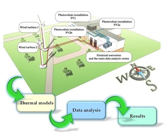
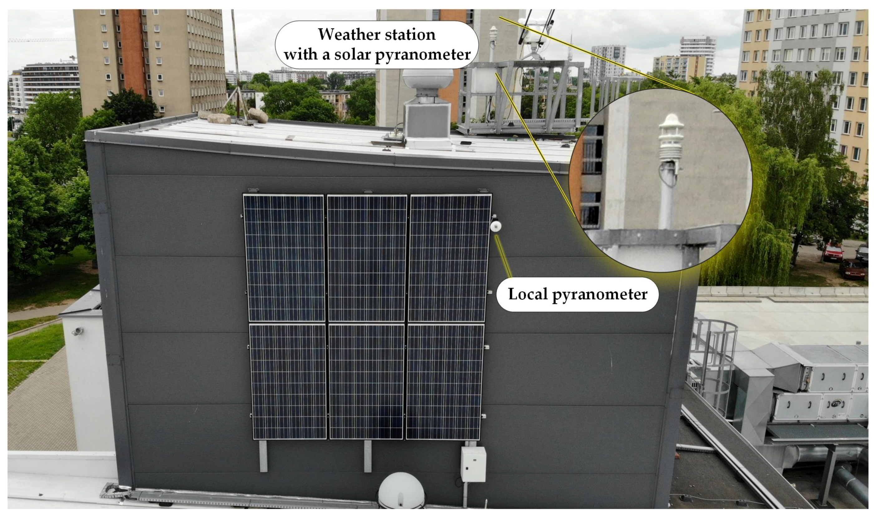
3. The Subject of the Research Description

Three photovoltaic installations being part of a hybrid power plant at the Bialystok University of Technology, Poland, initiated in 2015, are the subject of this research (Figure 1) [26]. The average annual irradiance value for the area of Bialystok in 2007–2016 was 1055 kWh/m², and the average annual insolation was 1758.7 h [27].

The effective work of the discussed photovoltaic power plant was only possible during sunny periods, i.e., when the sky was cloudless and in the period between dawn and dusk. The shortest operating period in Bialystok lasts only 7 h and 37 min, which is only 30% of a day. Whereas the longest operating period in the summer is 16 h and 58 min, which stands for 70% of a day. Moreover, in winter, many days in Bialystok are cloudy, which is the reason why the value of insolation in this town within the period from October to March is very low. In the summer, the number of sunny days is about 50% to 70%, while, in winter, it is only 20% to 25%. As a result, in winter, the period of effective work of a PV power plant in Bialystok is very short, and the values of generated energy are rather low [6]. For the purpose of this work, the following installations were analyzed.

PV1—a photovoltaic installation of the rated peak power of 3 kWp, located on the roof of the building of Bialystok University of Technology Academic Business Incubator. Figure 2 presents a photograph of the PV generator composed of 12 polycrystalline ESP 250 6P modules set in two rows and mounted optimally, which means towards the azimuth facing the south and with the slope angle of 38°. The modules are connected with an inverter produced by SMA (Niestetal, Germany), type SUNNY BOY 3000 HF, of the maximum power of 3.15 kWp DC.

PV2a—a photovoltaic installation of the rated peak power of 1.5 kWp (Figure 3). It is located on the south-east wall of the building of Bialystok University of Technology Academic Business Incubator. Its generator includes 6 ESP 250 6P polycrystalline modules mounted at the angle of 90° towards the ground level and with the azimuth angle of 160°. The electric energy processing (DC/AC) was executed with the use of a GoodWe (Suzhou, China) NS-1500 inverter of the maximum power of 1.8 kWp DC.

PV2b—a photovoltaic installation of the rated peak power of 1.5 kWp, which, similarly to installation PV2a, is composed of 6 ESP 250 6P polycrystalline modules connected to a GoodWe NS-1500 inverter of the maximum power of 1.8 kWp DC. Its location, however, is different, as the PV generator is mounted on the south-west wall of the same building at the angle of 90° to the ground level and the azimuth angle of 250°. The view of this installation is presented in Figure 4.

All the analyzed photovoltaic installations exploit identical polycrystalline ESP 250 6P modules produced by Europe Solar Production (Munich, Germany).

Table 1. A sheet of technical parameters of the photovoltaic module used in the analyzed arrays [28]. STC: standard test conditions and NOCT: nominal operating cell temperature.

Company	Europe Solar Production
Model	ESP 250 6P
Dimensions	1640 × 990 × 40
Electrical Data at STC
Module Efficiency ηSTC	15.3	%
Peak Power Watts Pmax,STC	250	Wp
Maximum Power Voltage Vmpp,STC	30.93	V
Maximum Power Current Impp,STC	8.08	A
Electrical Data at NOCT
Peak Power Watts Pmax,NOCT	182	Wp
Maximum Power Voltage Vmpp,NOCT	28.04	V
Maximum Power Current Impp,NOCT	6.49	A
Temperatures Ratings
Temperature Coefficient of Pmax (βSTC)	−0.46	%/°C
Temperature Coefficient of Open-Circuit Voltage VOC	−0.34	%/°C
Temperature Coefficient of Short-Circuit Voltage Isc	0.07	%/°C

and

Table 2. A datasheet of the technical parameters of the inverters used in installations PV1 [29], PV2a and PV2b [30].

Company	SMA Solar Technology AG		GoodWe
Model	Sunny Boy 3000 HF		GW 1500-NS
DC Input
Maximum Input Voltage	700	V	500	V
Minimum Input Voltage	175	V	80	V
Rated Input Voltage	530	V	360	V
MPP Voltage Range	210–560	V	80–450	V
Maximum Input Current	15	A	10	A
AC Output
Maximum Output Current	15	A	7.5	A
Rated Power at 230 V, 50 Hz	3000	W	1500	W
Maximum Apparent AC Power	3000	VA	1500	VA
Efficiency
Maximum efficiency ηmax	96.3	%	97.0	A
European weighted efficiency ηEU	95.4	%	96.0	W

contain the technical parameters of the modules and inverters installed in the described arrays.

The hybrid power plant of the Bialystok Technical University is also equipped with a specially created measurement system that records all important parameters of the photovoltaic panels and inverter performances, as well as the weather conditions.

Temperature and solar radiation measurements were conducted with the use of a distributed measurement system consisting of a central unit and measurement modules. The NI (National Instruments, Austin, TX, USA) PXIe-8108 measurement unit was equipped with an Intel^® Core™ 2 Duo T9400 2.53 GHz dual core processor and an 80 GB HDD. Additionally, extension modules enabling the analysis of current parameters of the hybrid power station were placed in it. However, the main aim of the central unit was acquiring data from the measurement modules attached to the photovoltaic panels PV1, PV2a and PV2b. The NI-9148 external measurement modules (8-Slot, Spartan-3 FPGA and Ethernet CompactRIO Chassis), which were situated at the photovoltaic panels, were attached to the central unit via a LAN network. The modules conducted measurements of the temperature parameters of the photovoltaic modules (NI-9213+ K-type thermocouples,

Table 3. The selected parameters of the measurement units used for temperature measurements of photovoltaic modules and for measuring the output voltage of the pyranometer sensor [32,33]. PV: photovoltaic.

Parameter	Measurement of PV Module Temperature NI-9213—Thermocouple Module, Voltage Measurement with Conversion to Temperature	Pyranometer Data Acquisition NI-9219—Universal Multipurpose Module, Voltage Measurement
Number of channels	16 thermocouple channels	4 analog input channels
Analog-to-digital converter (ADC) resolution	24 bits	24 bits
Type of ADC	Delta-sigma (with analog prefiltering)	Delta-sigma (with analog prefiltering)
Sampling rate	1 S/s	2 S/s
Gain error in high-resolution mode at −40 °C to 70 °C	0.07% typical, 0.15% maximum	0.3% typical, 0.4% maximum
Offset error in high-resolution mode at −40 °C to 70 °C	4 μV typical, 6 μV maximum	6 μV typical, 180 μV maximum
Other	Cold-junction compensation −40 °C to 70 °C 1.1 °C typical, 2.1 °C maximum	Stability of the gain drift ± 20 (ppm of reading/°C)

), as well as the global solar radiation (NI-9219 + LP PYRA 03 sensors,

Table 4. The selected parameters of the LP PYRA 03 pyranometer (Delta OHM, Caselle di Selvazzano, Italy) used in the measurement system [34].

Parameter	Value
Class	second (ISO 9060)
Typical sensitivity	10 μV/(W/m2)
Impedance	33–45 Ω
Measuring range	0 ÷ 2000 W/m2
Viewing Field	2π sr
Spectral Field	305–2800 nm
Operating temperature	−40 °C–80 °C

).

The temperature measurements of the photovoltaic modules were done by drilling a hole in the back surface of a module (Figure 5) and placing there a K-type thermocouple. This solution was considered to be sufficient, as the accuracy of the applied sensor was ±1.5 °C, and a small hole in the panel did not affect its mechanical structure.

Moreover, environmental parameters were also monitored with the use of a WS501-UMB (Lufft, Fellbach, Germany) meteorological station, which was connected to an NI PXIe-8108 computer through an RS485 interface. It should be mentioned that this compact weather station of a relatively good accuracy exploits the following technologies for the measurements of weather conditions: wind speed and direction—ultrasonic sensor, air temperature—negative temperature coefficient (NTC) thermistor, relative humidity (RH)—capacitive sensor, air pressure—microelectromechanical (MEMS) capacitive sensor and solar radiation—Kipp & Zonen (Delft, The Netherlands) pyranometer sensor [31].

The system of acquiring, storing, processing and visualizing the measurement data records and processes all information about the weather conditions, including the information concerning solar radiation, wind direction and speed, ambient temperature and the temperature of particular PV modules building the analyzed installation. The measured electrical and nonelectrical quantities are stored in a server with a database, and the current power plant performances are presented on a special website [26]. Selected environmental parameters and those related with the hybrid system performance are stored and shared for conducting calculations and scientific analysis. It is also possible to export the data as spreadsheet files, which enables precise data analysis in external software.

4. The Analysis of Average Monthly and Daily Estimated Temperatures of the PV Modules

The changing weather conditions have a significant impact on the performance of photovoltaic installations. The radiation intensity and the temperature of the PV modules are two main parameters that directly influence the amount of energy produced in a PV system. The biggest efficiency may be obtained through minimizing the temperature of a photovoltaic module and maximizing the insolation on its surface.

4.1. The Influence of Weather Conditions on the Operating Temperatures of PV Modules

The increase of irradiance is the main factor of the module power increase, but it also causes the increase of the operating temperature. This temperature value is also correlated with the ambient temperature, which can be seen in Figure 6. It presents the characteristics of the average observed monthly temperature of the PV1 modules, the ambient temperature and the wind speed during 2019. In order to determine the sheets presented below, the average monthly values of the parameters mentioned above, obtained from the data storage system of the Bialystok Technical University power plant, were used. The average measured monthly irradiance values in 2019 are presented in

Table 5. Average measured monthly values of the weather parameters and operating temperatures of the PV1 modules.

Month	Average Wind Speed vw (m/s)	Average Ambient Temperature Ta (°C)	Average Irradiance G0 (W/m2)	Average Operating Temperature Tmod (°C)
I	2.84	−3.27	120.20	1.24
II	3.20	2.71	208.06	8.88
III	3.90	5.74	339.05	15.08
IV	2.95	11.95	556.20	27.81
V	2.16	10.68	310.34	20.10
VI	2.84	23.48	592.94	39.75
VII	3.20	18.95	445.28	31.28
VIII	2.22	20.60	533.60	36.37
IX	3.20	15.73	458.14	28.17
X	2.40	10.76	280.39	18.98
XI	2.84	5.29	66.38	8.54
XII	2.44	2.67	81.77	5.99

. They are the highest in April, June and August. The analysis takes into account the working time of the installation only from 8 a.m. to 4 p.m., which enables avoiding a calculation error resulting from significant changes of the irradiance and the temperature values before sunrise and after sunset.

It can be observed in Table 5 that, in April and in September, the monthly average operating temperatures of the PV modules had similar values (about 28 °C); however, the weather parameters were slightly different. Comparing April to June, the monthly average values of the wind speed and the monthly average values of irradiance were approximately the same, but there was a significant difference in the average ambient temperature (about 12 °C). In turn, comparing April to August, the monthly average values of irradiance were similar, but there were significant differences in the wind speed (about 1 m/s lower in August) and in the ambient temperature (about 10 °C higher in August).

The average temperature of the PV modules rises with the increase of the average ambient temperature, whereas its dependence from the average wind speed is not noticeable. Describing the correlation between these two quantities is quite complicated because of the fact that the wind conditions change constantly.

4.2. The Parameters of Mathematical Models Found in the Literature

In the literature, we can find a few ways of parametrizing the connection between the temperature of the modules, irradiance, ambient temperature and the wind speed, and the most frequently used for this purpose formulas are presented in Section 2 of this paper.

Table 6. The juxtaposition of the parameters used in the calculations of the temperatures of the PV modules [10,11,18,19,21,22].

Model	Parameter		Value	Quantities
Faiman	U0		30.02	W·m−2·°C−1
	U1		6.28	W·s·m−3·°C−1
King	a	Stand-alone power system PV1	−3.56	-
		Building-integrated power systems PV2a and PV2b	−2.81
King	b	Stand-alone power system PV1	−0.0750	s·m−1
		Building-integrated power systems PV2a and PV2b	−0.0455
Skoplaki	$\omega$	Stand-alone power system PV1 (flat-roof)	1.2	-
		Building-integrated power systems PV2a and PV2b	2.4 (2.2-2.6)
Skoplaki 1 and 2		τ·α	0.90	-
Mattei 1 and 2			0.81

collects the values of the parameters occurring in the above-mentioned mathematical models.

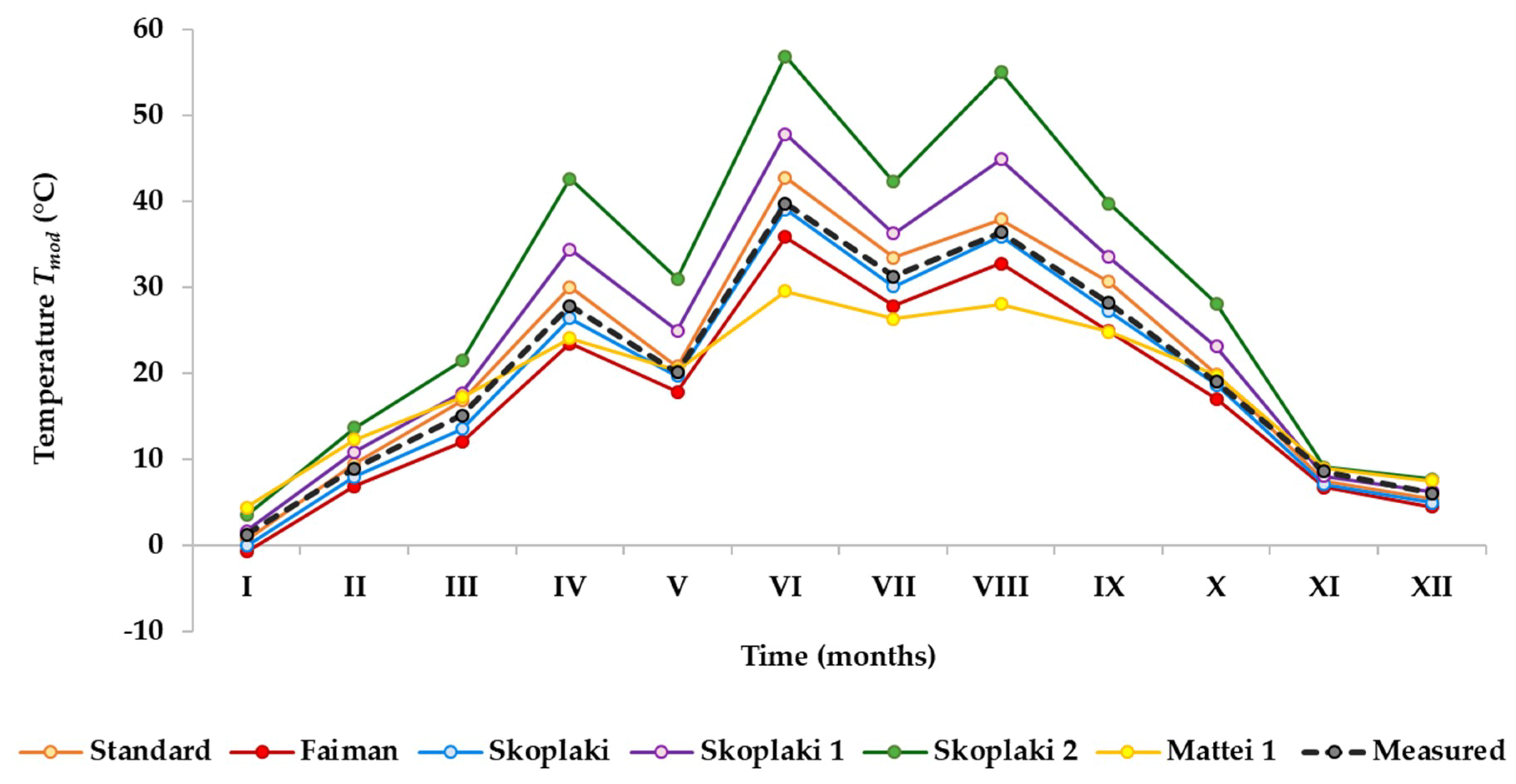
4.3. The Graphical Comparison of the Selected Models for Estimating the Temperatures of the PV Modules

Charts representing the average observed and estimated monthly and daily temperature values of the PV modules for installations PV1, PV2a and PV2b were determined. Figure 7, Figure 8 and Figure 9 present the effects of the analysis for the whole of 2019, while Figure 10, Figure 11 and Figure 12 show the results obtained for April and September of 2019. Lines of different colors represent the average values of the module temperatures determined with the use of mathematical models, whereas the black dotted line stands for the average values of the measured temperatures of the photovoltaic modules.

Analyzing the characteristics presented in Figure 10, we can notice that the average daily values of the module temperatures for installation PV1 closest to the measurement values were obtained with the use of the Skoplaki model (the measured values are about 2–5% higher than the estimated values). When the Faiman and the standard models were applied, the estimated values were similar to the observed ones, but the values obtained on the basis of the Mattei 1, Skoplaki 1 and Skoplaki 2 models were significantly different from them. It is visible in Figure 11 that, for installation PV2a, determining the values that are similar to the measured ones is possible due to conducting calculations using the Skoplaki 1 and the standard methods. The effects of the calculations done with the use of the Faiman and Mattei 1 models have too-low values in relation to the temperature values determined on the basis of the measurement data. According to the characteristics obtained from installation PV2b (Figure 12), the results obtained with the use of the standard method best reflect the values determined in the data storage system (the differences between them are 0.1–3.5 °C). Good results are also noted for the Skoplaki 1 method. The results of calculations conducted with the use of other mathematical models differ significantly from the observed temperature values.

4.4. Methodology and Data Analysis

The methodology is based on monthly and daily data averaging and using the normalized error measures. The normalized mean square error (NRMSE), normalized mean bias error (NMBE) and Pearson’s correlation coefficient k values were carried out in accordance with the following formulas [12]:

$$RMSE=\sqrt{\frac{{{\displaystyle \sum }}_{i=1}^n{(T_{modCi}-T_{{mod}_{Mi}})}^2}{n}},$$

(14)

$$NRMSE=\frac{RMSE}{{\overline{T}}_{modM}}100\%,$$

(15)

$$MBE=\frac{{{\displaystyle \sum }}_{i=1}^n\left(T_{modCi}-T_{{mod}_{Mi}}\right)}{n},$$

(16)

$$NMBE=\frac{MBE}{{\overline{T}}_{modM}}100\%,$$

(17)

$$k=\frac{{{\displaystyle \sum }}_{i=1}^n\left(T_{modCi}-{\overline{T}}_{modC}\right)\cdot \left(T_{{mod}_{Mi}}-{\overline{T}}_{modM}\right)}{\sqrt{\left[{{\displaystyle \sum }}_{i=1}^n{\left(T_{modCi}-{\overline{T}}_{modC}\right)}^2\right]\cdot \left[{{\displaystyle \sum }}_{i=1}^n{\left(T_{{mod}_{Mi}}-{\overline{T}}_{modM}\right)}^2\right]}},$$

(18)

where:

• $T_{modCi}$—the estimated value of the temperature,
• ${\overline{T}}_{modC}$—the average value of the estimated temperature,
• $T_{{mod}_{Mi}}$—the observed (measured) value of the temperature,
• ${\overline{T}}_{modM}$—the average value of the observed temperature,
• i—the summing index and
• n—the number of data used.

In the first part of the data analysis (

Table 7. The dataset of the normalized root mean square error (NRMSE), normalized mean bias error (NMBE) values and the Pearson’s correlation coefficient for the average monthly values of the module temperatures for the PV1, PV2a and PV2b installations calculated with the use of mathematical models during 2019. K: Pearson’s correlation coefficient.

	PV1			PV2a			PV2b
	NRMSE (%)	NMBE (%)	k (-)	NRMSE (%)	NMBE (%)	k (-)	NRMSE (%)	NMBE (%)	k (-)
Standard	8.27	5.31	1.00	20.16	−19.53	1.00	10.24	−8.05	1.00
Skoplaki	5.29	−4.87	1.00	7.95	1.92	1.00	16.93	10.49	0.99
Skoplaki 1	24.22	19.50	0.83	10.98	−10.39	0.86	9.00	−0.18	0.90
Skoplaki 2	53.39	44.96	0.99	12.07	6.06	0.99	20.60	14.03	0.99
Faiman/Koehl	14.53	−13.82	1.00	33.65	−31.93	1.00	19.35	−18.83	1.00
Mattei 1	22.72	−7.92	0.98	42.98	−33.49	0.98	40.48	−30.07	0.95
Mattei 2	22.60	−7.35	0.98	42.83	−33.19	0.98	40.56	−29.92	0.95
King	52.99	−47.89	0.98	58.09	−53.96	0.97	39.22	−37.92	0.99

), the average monthly values of the module temperatures in 2019, obtained with the use of the standard method, the Skoplaki, Skoplaki 1, Skoplaki 2, Faiman, Mattei 1, Mattei 2 and King models, were taken as estimated values. The measured average monthly values of the module temperatures of particular installations, determined on the basis on the data storage system, were taken as observed (measured) values. Due to the annual period of the analysis, the number of data used (estimated and corresponding observed) n was 12, whereas the values of the summing index i were consistent with the number of investigated months. The number of data points in a 30-day month was 122,000. The data was asynchronously acquired, the sampling rate was about eight per minute. The RAW data without filtration was used to create models. There were not unwanted spikes or missing data points in the datasets.

In the second part of the data analysis (

Table 8. The dataset of the NRMSE, NMBE values and the Pearson’s correlation coefficient for the average daily values of the module temperatures for the PV1, PV2a and PV2b installations calculated with the use of mathematical models in April, 2019.

	PV1			PV2a			PV2b
	NRMS E (%)	NMBE (%)	k (-)	NRMSE (%)	NMBE (%)	k (-)	NRMSE (%)	NMBE (%)	k (-)
Standard	12.75	7.99	0.96	20.44	−16.63	0.90	9.43	−6.81	0.97
Skoplaki	5.93	−4.92	0.99	14.49	10.30	0.97	20.34	17.88	0.96
Skoplaki 1	26.49	24.43	0.48	8.63	−5.44	0.52	8.73	3.76	0.56
Skoplaki 2	59.69	55.58	0.94	20.34	16.00	0.97	27.12	23.32	0.91
Faiman/Koehl	16.20	−15.67	0.99	34.29	−33.09	0.95	22.08	−21.25	0.97
Mattei 1	22.21	−15.48	0.98	41.39	−37.80	0.89	39.05	−34.85	0.88

,

Table 9. The dataset of the NRMSE, NMBE values and the Pearson’s correlation coefficient for the average daily values of the module temperatures for the PV1, PV2a and PV2b installations calculated with the use of mathematical models in June, 2019.

	PV1			PV2a			PV2b
	NRMS E (%)	NMBE (%)	k (-)	NRMSE (%)	NMBE (%)	k (-)	NRMSE (%)	NMBE (%)	k (-)
Standard	8.28	6.43	0.99	14.81	−13.93	0.98	8.27	−4.87	0.99
Skoplaki	3.01	−0.87	1.00	9.03	4.98	0.96	16.36	13.40	0.99
Skoplaki 1	24.20	22.48	0.98	7.77	−5.03	0.98	6.16	4.37	0.97
Skoplaki 2	52.01	48.56	0.96	13.92	9.79	0.94	24.22	18.72	0.98
Faiman/Koehl	9.64	−9.32	1.00	23.91	−23.31	0.98	15.47	−12.65	0.98
Mattei 1	29.87	−27.84	0.99	48.43	−47.28	0.77	47.33	−44.93	0.93

,

Table 10. The dataset of the NRMSE, NMBE values and the Pearson’s correlation coefficient for the average daily values of the module temperatures for the PV1, PV2a and PV2b installations calculated with the use of mathematical models in August, 2019.

	PV1			PV2a			PV2b
	NRMSE (%)	NMBE (%)	k (-)	NRMSE (%)	NMBE (%)	k (-)	NRMSE (%)	NMBE (%)	k (-)
Standard	7.16	3.67	0.98	17.95	−17.03	0.98	5.04	−3.76	0.99
Skoplaki	2.90	−0.46	1.00	12.73	8.34	0.97	18.28	15.99	0.98
Skoplaki 1	28.08	25.00	0.94	7.43	−3.02	0.92	9.23	7.06	0.93
Skoplaki 2	62.04	55.84	0.96	22.94	17.18	0.96	26.32	22.75	0.96
Faiman/Koehl	9.74	−9.50	1.00	26.63	−25.57	0.97	11.41	−10.56	0.98
Mattei 1	27.44	−24.50	0.98	46.13	−43.52	0.93	43.80	−40.68	0.82

,

Table 11. The dataset of the NRMSE, NMBE values and the Pearson’s correlation coefficient for the average daily values of the module temperatures for the PV1, PV2a and PV2b installations calculated with the use of mathematical models in September, 2019.

	PV1			PV2a			PV2b
	NRMSE (%)	NMBE (%)	k (-)	NRMSE (%)	NMBE (%)	k (-)	NRMSE (%)	NMBE (%)	k (-)
Standard	11.25	8.78	0.98	14.56	−12.70	0.97	6.44	−1.83	0.97
Skoplaki	3.75	−1.98	1.00	16.34	9.28	0.96	19.49	15.77	0.97
Skoplaki 1	26.14	21.69	0.56	9.96	−3.65	0.59	9.23	5.23	0.66
Skoplaki 2	54.78	46.42	0.96	22.23	13.59	0.93	23.92	19.15	0.96
Faiman/Koehl	11.32	−10.68	1.00	28.34	−26.21	0.94	14.62	−13.08	0.97
Mattei 1	21.84	−14.64	0.97	39.54	−34.61	0.89	37.03	−31.68	0.72

,

Table 12. The dataset of the NRMSE values for the average daily and monthly values of the module temperatures for the PV2a and PV2b installations calculated with the use of the Skoplaki model for mounting coefficient $\omega$ = 2.4 from the literature and for $\omega$ = 2 proposed by the authors.

	PV2a		PV2b
	NRMSE (%)	NRMSE (%)	NRMSE (%)	NRMSE (%)
	$\mathit{\omega }$	$\mathit{\omega }=2$	$\mathit{\omega }=2.4$	$\mathit{\omega }=2$
April	14.49	7.81	20.34	10.54
June	9.03	6.67	16.36	7.94
August	12.73	6.86	18.28	10.64
September	16.34	9.72	19.49	11.36
whole year 2019	7.95	8.41	16.93	10.24

and

Table 13. The dataset of the NMBE values for the average daily and monthly values of the module temperatures for the PV2a and PV2b installations calculated with the use of the Skoplaki model for mounting coefficient $\omega$ = 2.4 from the literature and for $\omega$ = 2 proposed by the authors.

	PV2a		PV2b
	NMBE (%)	NMBE (%)	NMBE (%)	NMBE (%)
	$\mathit{\omega }=2.4$	$\mathit{\omega }=2$	$\mathit{\omega }=2.4$	$\mathit{\omega }=2$
April	10.30	−1.69	17.88	7.07
June	4.98	−2.82	13.40	6.22
August	8.34	−0.99	15.99	8.68
September	9.28	−0.53	15.77	7.80
whole year 2019	1.92	−7.43	10.49	2.38

), the average daily temperature values in April, June, August and September of 2019 were taken as calculated values. The number of data used (estimated and corresponding observed) n was 30, and the values of the summing index i were consistent with the number of investigated days in a month. The number of data points in a day was 4066.

Summing up, the estimated average values of the module temperatures closest to the observed (measured) values in the case of installation PV1 were obtained with the use of the Skoplaki model (3); for installation PV2a, it was the Skoplaki (3) and Skoplaki 1 (5) models, whereas, for installation PV2b—the standard (1) and Skoplaki 1 (5) models. Applying other mathematical methods in the calculations leads to underestimating or overestimating the obtained values in relation to the values from the data storage system.

After many simulations, the authors observed that the value of the mounting coefficient $\omega$ representing the ventilation effect in the Skoplaki model, which in the literature is advised as 2.4 for facade-integrated installations, could be lower. The most optimal value for both the PV2a and PV2b installations is 2. This confirms the NMRSE and NMBE values presented in Table 12 and Table 13, which are lower for $\omega$ = 2 in the datasets from April, June, August and September.

4.5. The Impact of Wind Speed

An additional verification of the mathematical models was performed in

Table 14. The differences between the average observed and estimated module temperatures at two average wind speeds on 24 August 2019 and 28 August 2019 (from 8 a.m. to 4 p.m.).

Installation Name and Date	Faiman	Skoplaki	Skoplaki*	Skoplaki 1	Mattei 1	Wind Speed	Module and Ambient Temp.	Irradiance
	${\overline{\mathit{T}}}_{\mathit{d}\mathit{i}\mathit{f}\mathit{f}}$ (°C)	${\overline{\mathit{T}}}_{\mathit{d}\mathit{i}\mathit{f}\mathit{f}}$ (°C)	${\overline{\mathit{T}}}_{\mathit{d}\mathit{i}\mathit{f}\mathit{f}}$ (°C)	${\overline{\mathit{T}}}_{\mathit{d}\mathit{i}\mathit{f}\mathit{f}}$ (°C)	${\overline{\mathit{T}}}_{\mathit{d}\mathit{i}\mathit{f}\mathit{f}}$ (°C)	${\overline{\mathit{v}}}_{\mathit{w}}$ (m/s)	${\overline{\mathit{T}}}_{\mathit{m}\mathit{o}\mathit{d}\mathit{M}};{\overline{\mathit{T}}}_{\mathit{a}}$ (°C)	${\overline{\mathit{G}}}_0$ (W/m2)
PV1: 24 Aug.	4.3	−1.4	−1.4	−18.4	17.6	1.0	47.9; 22.8	755.5
PV1: 28 Aug.	3.1	−1.1	−1.1	−12.6	13.6	2.7	44.5; 25.4	750.5
PV2a: 24 Aug.	13.1	−9.0	−3.0 ($\omega$= 2)	−2.5	26.8	1.0	50.1; 22.8	518.6
PV2a: 28 Aug.	9.9	−7.5	−2.7 ($\omega$= 2)	−1.2	21.9	2.7	46.8; 25.4	534.7
PV2b: 24 Aug.	3.1	−10.2	−6.6 ($\omega$= 2)	−6.3	17.2	1.0	34.4; 22.8	311.8
PV2b: 28 Aug.	5.0	−5.0	−2.2 ($\omega$= 2)	−1.4	18.6	2.7	37.0; 25.4	315.7

. It was based on two datasets that were acquired on two sunny days of August 2019. Two days when the values of the average irradiance G were similar but the wind speeds v_m were significantly different (1 m/s vs. 2.7 m/s) were chosen. The smallest differences between the average observed and estimated module temperatures (${\overline{T}}_{diff}={\overline{T}}_{modM}–{\overline{T}}_{modC}$) were obtained for the Skoplaki* model with a modified mounting coefficient (PV1: $\omega$ = 1.2 and PV2a and PV2b: $\omega$ = 2). It proved to be a good model for all installations. The Skoplaki 1 model is equally well-fitting in the case of the PV2a and PV2b installations. Tolerable results are also reported for the Faiman model with the parameters proposed by Koehl. However, the Mattei 1, 2 and the King models are poorly fitting for the parameters from Table 6.

5. Conclusions

Photovoltaic installations PV1, PV2a and PV2b, belonging to a hybrid power plant at the Bialystok University of Technology, were subject to the research. A precise analysis of the real influence of weather conditions, obtained during long-term measurements, enabled to learn in detail the behavior of the arrays in changeable and unpredictable environmental conditions that have occurred lately in Poland. Due to that, for the purpose of the presented research, tests concerning the dependence of the PV system operating temperatures on the weather conditions, with a special concern for the wind speed, were conducted on the basis of the collected measurement data and mathematical models. For this purpose, different mathematical models: King, Skoplaki, Skoplaki 1, Skoplaki 2, Faiman, Mattei 1 and Mattei 2 and the standard model were analyzed. They enabled to determine the operating temperatures of photovoltaic modules with weather conditions, including wind, taken into consideration. Average values of the ambient temperature, wind speed and the irradiance for the tested installations in 2019 obtained from the data storage system of the university power plant were used to conduct the calculations. The graphs created as a result of the tests showed the characteristics of the temperature mean value changes for the PV1, PV2a and PV2b installations.

On the basis of the conducted analysis, it can be stated that it is hard to choose a general theoretical model for determining the operating temperature of the PV modules that would be relevant for each installation. In the case of a detached array (PV1), the Skoplaki model appeared to be the best one (NRMSE was 6% maximum and NMBE—5% maximum; see Table 7, Table 8, Table 9, Table 10 and Table 11). Whereas, for the installation PV2b mounted on the south-west wall, the values obtained from the data storage system were better expressed by the standard model (NOCT) and the Skoplaki 1 model. In the case of the NOCT model, the NRMSE was 10% maximum and the NMBE—8% maximum. In turn, the Skoplaki and Skoplaki 1 models were more suitable for installation PV2a (on the south-east wall). The error values were slightly higher—the maximum NRMSE was 11% (Skoplaki 1) and 16% (Skoplaki). This may result from variations in the ventilation of the modules for various types of mountings of the installations. In the detached systems, the blowing wind has a positive influence on the modules’ work, because it receives the heat excess from their back surfaces. However, in the installations mounted on a facade, it is not possible, because the air flow is limited by the wall of the building.

The results of the conducted analysis (Table 14) confirm a significant influence of the cooling effect, which naturally decreases the operating temperature of the PV modules and improves the negative influence of the temperature increase on their operating parameters. A good cohesion of the results of the calculations based on the Skoplaki model with the observed measurement data proves the need to consider also the influence of the wind speed while determining the operating temperature of photovoltaic detached installations. The mounting issue is essential as well. Based on earlier observations of the accuracy measures, the authors of this paper proposed a lower value of the mounting coefficient $\omega$ than in the literature that was more relevant for the PV2a and PV2b facade-based installations. After this modification, there was a significant decrease of the NRMSE and the NMBE values (Table 12 and Table 13).

The average daily values of the errors were larger than the values given by the authors of publication [10]. In this publication, 15 min, hourly and daily RMSE values were presented for different panel technologies. Moreover, the RMSE measure was used, and the presented results varied from 2 °C to 7 °C for the polycrystalline (p-Si) panels, i.e., from 5.7% to 20% at 35 °C. We decided to use the normalized NRMSE measure, which is related to the average operating temperature of PV panels. The achieved results were up to 62% (Table 10). For the Skoplaki model, it was 6% (PV1), 10% (PV2a) and 11% (PV2b) maximums. This model was the most suitable for the studied PV system configurations.

References

1. Alazab, M.; Khan, S.; Krishnan, S.S.R.; Pham, Q.V.; Reddy, M.P.K.; Gadekallu, T.R. A multidirectional LSTM model for predicting the stability of a smart grid. IEEE Access 2020, 8, 85454–85463. [Google Scholar] [CrossRef]
2. Markvart, T. (Ed.) Solar Electricity, 2nd ed.; Wiley: Hoboken, NJ, USA, 2000; ISBN 978-0-471-98852-6. [Google Scholar]
3. Petrone, G.; Ramos-Paja, C.A.; Spagnuolo, G.; Xiao, W. Photovoltaic Sources Modeling; John Wiley & Sons, Inc.: Hoboken, NJ, USA, 2015; ISBN 9781118679036. [Google Scholar]
4. Xiao, W. Photovoltaic Power System: Modeling, Design, and Control; Wiley: Hoboken, NJ, USA, 2017; ISBN 9781119280347. [Google Scholar]
5. Gökmen, N.; Hu, W.; Hou, P.; Chen, Z.; Sera, D.; Spataru, S. Investigation of wind speed cooling effect on PV panels in windy locations. Renew. Energy 2016, 90, 283–290. [Google Scholar] [CrossRef]
6. Kusznier, J.; Wojtkowski, W. Impact of climatic conditions on PV panels operation in a photovoltaic power plant. In Proceedings of the 15th Selected Issues of Electrical Engineering and Electronics, WZEE 2019, Zakopane, Poland, 8–10 December 2019. [Google Scholar]
7. Nkurikiyimfura, I.; Safari, B.; Nshingabigwi, E. A simulink model of photovoltaic modules under varying environmental conditions. IOP Conf. Ser. Earth Environ. Sci. 2018, 159, 012024. [Google Scholar] [CrossRef] [Green Version]
8. Perovic, B.; Klimenta, D.; Jevtic, M.; Milovanovic, M. A transient thermal model for flat-plate photovoltaic systems and its experimental validation. Elektronika Ir Elektrotechnika 2019, 25, 40–46. [Google Scholar] [CrossRef] [Green Version]
9. Mora Segado, P.; Carretero, J.; Sidrach-de-Cardona, M. Models to predict the operating temperature of different photovoltaic modules in outdoor conditions. Prog. Photovolt. Res. Appl. 2015, 23, 1267–1282. [Google Scholar] [CrossRef]
10. Schwingshackl, C.; Petitta, M.; Wagner, J.E.; Belluardo, G.; Moser, D.; Castelli, M.; Zebisch, M.; Tetzlaff, A. Wind effect on PV module temperature: Analysis of different techniques for an accurate estimation. Energy Procedia 2013, 40, 77–86. [Google Scholar] [CrossRef] [Green Version]
11. Veldhuis, A.J.; Nobre, A.; Reindl, T.; Ruther, R.; Reinders, A.H.M.E. The influence of wind on the temperature of PV modules in tropical environments, evaluated on an hourly basis. In Proceedings of the IEEE Photovoltaic Specialists Conference, Tampa, FL, USA, 16–21 June 2013. [Google Scholar]
12. Frydrychowicz-Jastrzebska, G.; Bugała, A. Modeling the distribution of solar radiation on a two-axis tracking plane for photovoltaic conversion. Energies 2015, 8, 1025–1041. [Google Scholar] [CrossRef]
13. Armstrong, S.; Hurley, W.G. A thermal model for photovoltaic panels under varying atmospheric conditions. Appl. Eng. 2010, 30, 1488–1495. [Google Scholar] [CrossRef]
14. Chen, J.L.; He, L.; Yang, H.; Ma, M.; Chen, Q.; Wu, S.J.; Xiao, Z. Empirical models for estimating monthly global solar radiation: A most comprehensive review and comparative case study in China. Renew. Sustain. Energy Rev. 2019, 108, 91–111. [Google Scholar] [CrossRef]
15. Idzkowski, A.; Walendziuk, W.; Borawski, W. Analysis of the temperature impact on the performance of photovoltaic panel. In Proceedings of the SPIE—The International Society for Optical Engineering; Romaniuk, R.S., Ed.; International Society for Optics and Photonics: Bellingham, WA, USA, 2015; Volume 9662, p. 96620. [Google Scholar]
16. Kandemir, E.; Borekci, S.; Cetin, N.S. Conventional and soft-computing based MPPT methods comparisons in direct and indirect modes for single stage PV systems. Elektronika Ir Elektrotechnika 2018, 24, 45–52. [Google Scholar] [CrossRef] [Green Version]
17. Jaszczur, M.; Teneta, J.; Hassan, Q.; Majewska, E.; Hanus, R. An experimental and numerical investigation of photovoltaic module temperature under varying environmental conditions. Heat Transf. Eng. 2019. [Google Scholar] [CrossRef]
18. Skoplaki, E.; Boudouvis, A.G.; Palyvos, J.A. A simple correlation for the operating temperature of photovoltaic modules of arbitrary mounting. Sol. Energy Mater. Sol. Cells 2008, 92, 1393–1402. [Google Scholar] [CrossRef]
19. Mattei, M.; Notton, G.; Cristofari, C.; Muselli, M.; Poggi, P. Calculation of the polycrystalline PV module temperature using a simple method of energy balance. Renew. Energy 2006, 31, 553–567. [Google Scholar] [CrossRef]
20. Faiman, D. Assessing the outdoor operating temperature of photovoltaic modules. Prog. Photovolt. Res. Appl. 2008, 16, 307–315. [Google Scholar] [CrossRef]
21. King, D.L.; Boyson, W.E.; Kratochvil, J.A. Photovoltaic array performance model. Sandia Rep. 2004, 8, 1–41. [Google Scholar] [CrossRef] [Green Version]
22. Koehl, M.; Heck, M.; Wiesmeier, S.; Wirth, J. Modeling of the nominal operating cell temperature based on outdoor weathering. Sol. Energy Mater. Sol. Cells 2011, 95, 1638–1646. [Google Scholar] [CrossRef]
23. Kurtz, S.; Whitfield, K.; Miller, D.; Joyce, J.; Wohlgemuth, J.; Kempe, M.; Dhere, N.; Bosco, N.; Zgonena, T. Evaluation of high-temperature exposure of rack-mounted photovoltaic modules. In Proceedings of the 34th IEEE Photovoltaic Specialists Conference, Philadelphia, PA, USA, 7–12 June 2009. [Google Scholar]
24. Mavromatakis, F.; Kavoussanaki, E.; Vignola, F.; Franghiadakis, Y. Measuring and estimating the temperature of photovoltaic modules. Sol. Energy 2014, 110, 656–666. [Google Scholar] [CrossRef]
25. HOMER Energy. How HOMER Calculates the PV Array Power Output. Available online: https://www.homerenergy.com/products/pro/docs/latest/how_homer_calculates_the_pv_array_power_output.html (accessed on 13 June 2020).
26. Bialystok University of Technology. Hybrid Power Plant of the Bialystok University of Technology. Available online: http://elektrownia.pb.edu.pl/ (accessed on 13 June 2020).
27. European Commission. JRC Photovoltaic Geographical Information System (PVGIS)—European Commission. Available online: https://re.jrc.ec.europa.eu/pvg_tools/en/tools.html (accessed on 13 June 2020).
28. Europe Solar Production. Polycrystalline Photovoltaic Module Europe Solar Production Premium Quality Solar Module Data Sheet ESP 6P 240-255 Wp. Available online: http://europe-solarproduction.com/media/690/ESP-Polycrystalline-Solar-Module-Datasheets-ESP-6P-series.pdf (accessed on 17 August 2020).
29. SMA Solar Technology AG. SUNNY BOY 2000HF/2500HF/3000HF—Installation Guide. Available online: https://www.solartradesales.co.uk/Cache/Downloads/SunnyBoy-HF-Installation-guide-3.pdf (accessed on 17 August 2020).
30. Solahart Goodwe Single Phase Small Domestic Inverter. GW1500-NS & GW3000-NS. Available online: https://www.solahart.com.au/media/5305/ih0113_gw1500-ns-gw3000-ns_single-phase-inverters_june-2019_web.pdf (accessed on 13 June 2020).
31. Compact Weather Sensors—WS501-UMB Smart Weather Sensor. Available online: https://www.lufft.com/products/compact-weather-sensors-293/ws501-umb-smart-weather-sensor-1839/ (accessed on 24 July 2020).
32. National Instruments. NI 9213 Datasheet. Available online: https://www.ni.com/pdf/manuals/378021a_02.pdf (accessed on 24 July 2020).
33. National Instruments. NI 9219 Datasheet. Available online: https://www.ni.com/pdf/manuals/377223a_02.pdf (accessed on 24 July 2020).
34. Delta OHM. LP Pyra 02—LP Pyra 03—LP Pyra 12. Available online: https://www.deltaohm.com/ver2012/download/LP_PYRA02_03_12_uk.pdf (accessed on 24 July 2020).
Figure 1. The general scheme of the hybrid power plant at the Bialystok University of Technology, where: WT1 and WT2—wind turbines, PV1—optimal located photovoltaic installation, PV2a and PV2b—wall-mounted photovoltaic installations, PV3—tracker photovoltaic installation (not analyzed in this paper), WS—weather station and EC&DC—electrical converters and the main data analysis center.
Energies 13 04274 g001
Figure 2. A view of a photovoltaic installation with panels set optimally.
Energies 13 04274 g002
Figure 3. A view of the photovoltaic installation on the south-east wall.
Energies 13 04274 g003
Figure 4. A view of the photovoltaic installation on the south-west wall.
Energies 13 04274 g004
Figure 5. A view of the thermocouple sensor location in photovoltaic modules.
Energies 13 04274 g005
Figure 6. The characteristics of the average observed monthly temperature of the PV1 installation modules, the ambient temperature and the wind speed in 2019.
Energies 13 04274 g006
Figure 7. The characteristics of the average observed and estimated monthly values of the module temperatures of the PV1 installation in 2019.
Energies 13 04274 g007
Figure 8. The characteristics of the average observed and estimated monthly values of the module temperatures of the PV2a installation in 2019.
Energies 13 04274 g008
Figure 9. The characteristics of the average observed and estimated monthly values of the module temperatures of the PV2b installation in 2019.
Energies 13 04274 g009
Figure 10. The characteristics of the average observed and estimated daily values of the module temperatures of the PV1 installation in September of 2019.
Energies 13 04274 g010
Figure 11. The characteristics of the average observed and estimated daily values of the module temperatures of the PV2a installation in September of 2019.
Energies 13 04274 g011
Figure 12. The characteristics of the average observed and estimated daily values of the module temperatures of the PV2b installation in September of 2019.
Energies 13 04274 g012