Abstract
Aggregated Norton’s equivalent models, with parallel impedance and current injection at different harmonic frequencies are used to model the distribution grid in harmonic studies. These models are derived based on measurements and/or prior knowledge about the grid. The measurement-based distribution (sub-)grid impedance estimation method uses harmonic phasors of 3-phase current and voltage measurements to capture the response of the distribution (sub-)grid before and after an event in the utility side of the grid. However, due to increasing non-linear components in the grid, knowledge about uncertainty in parameters of such equivalent models which intrinsically describe a linear grid becomes important. The aim of this paper is to present two novel methods to calculate the uncertainty of the measurement-based Norton’s equivalent harmonic model of the distribution (sub-)grids as seen from the utility side at the Point of Common Coupling (PCC). The impedance and the uncertainty calculations are demonstrated on a simulated network.
1. Introduction
To provide sustainable electricity supply to its customers, the Medium Voltage (MV) and Low Voltage (LV) distribution grids are witnessing a rapid increase in clean-energy sources (Wind Parks (WP), Photo-voltaic (PV) systems) and loads such as Battery Energy Storage Systems (BESS) and Electric Vehicle (EV) chargers. Inclusion of such power electronics connected sources and loads along with the increasing amount of cables in medium and low voltage networks are causing a change in the impedance of the distribution (sub-)grids. Harmonic current injections due to the increasing use of power electronic connected loads and generation sources result in increase in the voltage distortion at the Point of Common Coupling (PCC) which propagates in the grid. For analysis of harmonic distortion emissions and propagation, grid utilities are becoming more interested in new methods for harmonic state estimation, harmonic source localization and assessment of harmonic pollution contribution by the loads on the customer side [1]. Aggregated (sub-)grid models are required to perform and improve the accuracy of such investigations.
The impact of load models on harmonic impedance as seen from the transmission network was studied in [2]. The study showed that MV cables have a major influence on the harmonic impedance. It was concluded that it is important to model the transformers and cables of the MV network. Harmonic interaction between multiple distributed power inverters in a distribution network was studied in [3]. The authors of [4] investigated in detail the effect of modeling MV and LV network and components on the resonant frequencies and corresponding peaks. The effect of various load types on the relationship between grid frequency and impedance values was presented. It was shown that (sub-)grid impedance parameters should not be calculated from the power measurements at the fundamental frequency. The most prominent effect in the impedance is due to the equivalent capacitance of the household appliances and the PV inverters [3]. A simulation study performed by authors in [5] showed a resonance located at a very low frequency (500 Hz) in a residential grid which was caused by the power-electronics equipment used in the households.
It is very challenging for a network operator to know the exact composition of loads and sources connected to the grid at both MV and LV levels. Hence the estimation of system harmonic impedance relies on the aggregated load and network models. Loads in distribution grids are traditionally represented by the resistance and the reactance values calculated based on the measured active (P) and reactive (Q) power. These values, however, cannot be used directly to represent them for harmonic analysis.
Non-invasive measurement methods based on naturally occurring grid events have been used in the past to determine the (sub-)grid impedance [6,7,8,9,10]. These methods utilize events happening in the region outside the (sub-)grid to be modeled as a source of perturbation in harmonic voltages and measure the (sub-)grid’s response in terms of harmonic currents. Non-invasive measurements are different from invasive measurements presented in [11,12] where additional perturbation is injected into the (sub-)grid to perform such analysis. However, such opportunities to artificially perturb the grid at will and with desired magnitude and frequency spectrum could be rare or impossible. As suggested in [13], switching operations of transformers and capacitor banks could result in rich voltage spectra which would cause a current response from the (sub-)grid to be modeled. By measuring the change in the state of voltage at different harmonics and the response in terms of change in the current harmonics, a simplified impedance based on the linear Norton’s or Thevenin’s equivalent model of the distribution grid is achieved.
One major drawback in the non-invasive measurement-based impedance estimation methods presented in the literature is the lack of the information over the uncertainty of the estimated impedance values. As the modern distribution grid becomes more complex and non-linear, uncertainty associated with the impedance parameters of the used linear models must be evaluated. Authors in [14] presented a Monte Carlo simulation-based method to determine the uncertainty of the impedance using probability distribution for resistive, inductive and capacitive parameters of various loads. However, these parameters were varied based on the prior knowledge of the customer load profiles. Measurement-based methods do not need such prior knowledge and assumptions about the load and give results treating the unknown grid as a black-box. This paper presents two new methods to evaluate the uncertainty such measurement-based impedance parameters for a section of the distribution grid.
The rest of the paper is presented as followed: Section 2 presents the impedance identification method using non-invasive measurements. Section 3 presents the two proposed methods to evaluate the uncertainty in the estimated impedance. In Section 4, models of a linear distribution grid and a sub-grid with non-linear loads whose impedance needs to be estimated are presented. The results are discussed in Section 5. In the end, a discussion about the presented methods is presented in Section 6 and conclusions are drawn in Section 7.
2. Impedance Estimation
In this paper Norton’s equivalent circuit as shown by the Figure 1 is used to model the distribution grid which is modeled as a linear time invariant (LTI) system using a component-based design. Norton’s and Thevenin’s equivalent models are commonly used for harmonic analysis purposes [15]. Customer’s side impedance () and current injection () are the unknown parameters of this model. However, due to the increasing non-linearity in the distribution network, the generalization property of the assumed LTI model is weakened.
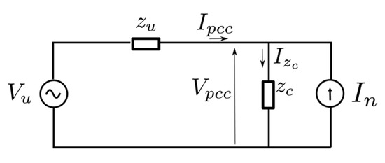
Figure 1.
Linear Norton’s equivalent model of the customer side distribution grid.
To determine the impedance of the distribution (sub-)grid, two states (pre-event and post-event) of the grid are used. Voltage and current signals are measured and then could either be converted into symmetrical (positive, negative and zero) sequence components using Park’s transformation or , and 0 components using Clarke’s transformation. After conversion, short time Fourier transform (STFT) is applied to the signals to calculate harmonic phasors of the signals over sliding time windows. The process of phasors estimation using STFT utilizes short duration blocks of data (10 cycles according to International Electrotechnical Commission (IEC) standard 61000-4-7 [16]) which allows for assumption that the signal’s frequency, phase and magnitude is not varying for the duration of the block. Using the calculated harmonic phasors, the impedance of the grid can be calculated as [6]:
where, and denote the states after and before the event and denotes the harmonic order. For multiple excited states, a linear regression model was used to estimate the impedance. Using the calculated customer’s side distribution grid impedance and the voltage and current phasors at the PCC, the current injection from the customers side () can be calculated as:
3. Proposed Uncertainty Estimation Methods
The paper proposes two methods to estimate the uncertainty in the impedance of the Norton’s equivalent model of the aggregated distribution grid. The first method (henceforth called the voltage distortion comparison (VDC) method) is based on the comparison of the calculated harmonic distortion caused by the customer at the PCC. The second method (henceforth called the current injection comparison (CIC) method) is based on the comparison of the harmonic current injection values calculated from pre- and post- event measurements using the calculated impedance .
3.1. Voltage Distortion Comparison
The contribution of voltage harmonic distortion caused by the customer’s side at the PCC can be calculated using two methods: the voltage harmonic vector (VHV) method is presented in [17] and the IEC voltage phasor method is presented in [18]. A description and comparison of these methods is presented in [19,20].
The VHV method uses the Thevenin’s equivalent circuit to calculate the customer’s contribution. Using the superposition principle of circuit theory, the harmonic contribution at the PCC from the customer’s side ( can be represented by the voltage drop caused by the customer’s voltage on the utility impedance and is given by:
where , and are the utility impedance, customer impedance and the Thevenin’s voltage at any given harmonic order at the customer’s end. From now and henceforth, the notation has been eliminated while all the following functions still give results for different harmonic orders. can be calculated using the estimated values of the Norton’s equivalent model and Equation (3) can be written as:
Utilizing Equations (3) and (4), the harmonic contribution function can be written as a function of form 9 with being the independent variable as:
IEC method also uses the Thevenin’s equivalent to calculate the contribution from the customer’s side. However, the contribution () is given by:
where,
is the harmonic voltage measured at the PCC and is the background voltage distortion caused by the interaction of loads and other components in the customer’s (sub-)gird and the rest of the network.
The major difference between the two methods is that the VHV method requires the knowledge of both the customer’s and the utility’s impedance, while the IEC method require only the utility impedance. The customer’s impedance () is estimated using Equation (1) after a recorded event and the utility impedance at the PCC () is provided by the utility. According to [19] both methods provide qualitatively correct emission contribution while the authors in [20] propose that for valid circuit model assumptions, the VHV method would give true harmonic emission contribution.
The proposed method to find the uncertainty in the estimates is based on comparing the difference in the distortion contribution (emission) calculated by the VHV and IEC methods. The difference () calculated using the available and values in Equations (5) and (6) is given by:
is taken as the maximum error in the value (2 standard deviations in the calculated value) given by Equation (4). It was also taken that the source of this error is the uncertainty in the variable . The variance in is then calculated using the error propagation theory of complex numbers and functions presented in [21,22].
For any complex function
the function can be written to be comprised of two scalar functions, and which give the real and imaginary parts such that
where, the variable X denotes the complex quantity + j. For 1 independent variable, the 2 × 2 covariance matrix of the estimate of X is given by:
The covariance matrix for the single output variable can be calculated using the generalized law of propagation of uncertainty. For a function given by Equation (9), the covariance of the output () can be calculated as:
where, is the sensitivity matrix given by:
For any complex quantity, , mapping
generates a matrix representation for Z that behaves as complex numbers under arithmetic operations such as division and multiplication [22]. Using the mapping , the sensitivity matrix can be expressed as [21]:
Using Equation (12), the diagonal elements of the covariance matrix is populated by the . For each harmonic order, the value was taken as the maximum error in the value for a normal distribution. The expected variance in the is then calculated using Equation (12) as:
Equation (16) gives the expected variance in the real and imaginary components of the customer impedance. An expansion factor of 2 was multiplied to the standard deviation () to calculate the total uncertainty envelope in real and imaginary parts of the calculated impedance (.
3.2. Current Injection Comparison
This method compares the harmonic current injection values calculated from pre- and post-event voltage and current measurements at the PCC using the estimated impedance () value in Equation (2). The measurement for voltage and current before and after the events are performed at the PCC. Using the Kirchoff’s current law,
Using Equation (17) in Equation (1),
where and are the assumed Norton’s injection current before and after the event. On comparing 1 and 18, it can be observed that:
If the difference in the Norton current injection can be written as:
then Equation (18) can be written as:
Thus, the sensitivity of the function given by Equation (21) to values (which is a constant parameter for a Norton’s equivalent model) is an indicator for uncertainty in the estimates. Equations (12) and (15) are followed to calculate the uncertainty in the given the variance in the .
The proposed methods are demonstrated to find the uncertainty of the impedance of a simulated distribution grid.
4. Distribution Grid Model
This section presents the simulated distribution grid to demonstrate the two proposed methods. Section 4.1 presents an aggregated model of a completely linear grid with multiple MV/LV transformers. In Section 4.2, power electronics based non-linear loads are added at one of the MV/LV transformers (called as sub-grid) to study the uncertainty in the impedance results caused by non-linear devices.
4.1. Aggregated Linear Model
To estimate the impedance of the distribution grid, a component-based system model of the network was selected and modeled in PSCAD software. Examples for modelling of the distribution grid for harmonic analysis are presented in [23,24]. Similar aggregated models have been used by other researchers to represent the distribution grid for harmonic studies [2,25]. The distribution network was modeled as per the recommendations in [24]. The network specifications were based on typical Dutch MV-LV distribution grids [26]. The aggregated distribution grid model along with two parallel transformers at the primary substation is shown in the Figure 2. L_MV and C_MV are the inductance and capacitance caused by the MV/LV transformers and MV cables. L_mot is the inductance of motors in the LV grid, C_LV2 is the aggregated capacitance of the household devices and R_LV2 is the resistance components of the loads.
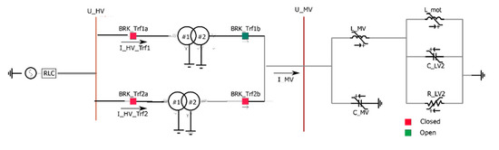
Figure 2.
Distribution grid seen from the HV side.
The voltage level of the High Voltage (HV) grid was 110 kV and the primary substation has two 110–10 kV transformers with nominal power rating () of 66 MVA. The upstream grid was modeled as a voltage source. The short circuit level of the grid at the 110 kV side of the transformers was 3000 MVA thus making it a strong grid. The transformers were modeled identically using the classical approach as described in [27]. The positive sequence leakage reactance () was set to be 0.1 p.u. and the air core reactance was set twice of at 0.2 p.u. Magnetizing current () was set to be 2 of the nominal current. Copper loss () and iron loss () were set to be 0.01 and 0.002 p.u. respectively. Saturation curve of the transformer is dependent on the air core reactance, magnetizing current and the knee point voltage which was set at 1.2 p.u. of the base voltage. The MV-LV transformers were modeled with their positive sequence leakage reactance while the copper and iron losses were ignored. The complete set of parameters for the modeled transformers are mentioned in the Table 1.

Table 1.
Transformer Models.
Representation of loads using the P and Q values from load flow analysis cannot be used to for harmonic analysis because active power absorbed by the rotating machines does not exactly correspond to a damping value. Hence aggregate load models of the network were modeled based on types mentioned in [13,24]. The resistive part of the load was aggregated as constant impedance load and the effective resistance was calculated based on the power consumption. Using a factor representing an estimated share of motor load in the total power demand, the impedance values were calculated as:
where, is the total megawatt demand, is the fraction of motor load in the total kW load, is the locked rotor reactance in p.u. and is the install factor of the motors. The typical values for ranges between 0.15 and 0.25 p.u., the typical install factor is 1.2. For the current model, was assumed to be 0.2 p.u. It is to be noted that, this model does not include the harmonic attenuation and is best suitable for moderate participation of induction motors (K < 0.3). For higher participation of motor loads (K > 0.7) such as in an industrial grid, then a more accurate representation includes a resistor in series with the inductance.
One of the important components to model is the capacitive effect of household appliances and solar inverters. As presented in [3], both can be represented by a capacitance value based on the power factor correction capacitors. The typical range for capacitance for household appliances is between 0.6 and 6 μF. A mean value of 3 μF was chosen for this study. An additional 0.5 to 10 μF could be added per household for inverters of 1–3 kW output range. It was also assumed that 25% of household have solar inverters and the mean value of the inverter output capacitance as 5 μF.
Total power demand of the distribution network was about 52.6 MVA. The MV and LV feeders in the Dutch grid are cables and are represented as constant capacitors. The capacitance was calculated based on the type and length of the feeders. From the primary substation there were 10 numbers of MV feeder of underground cable supplying to 20 MV-LV transformers. Each MV feeder was about 12 km long using a 3-core cable with a capacitance of 0.37 μF per km. Each MV-LV transformer was had an average of 5 feeders of an average 0.5 kM length with a capacitance of 1.26 μF per km and feeding 50 customers. Using the diversity factor of 0.1, the average demand per house was 1 kVA.
A complete summary of all the load and network components is presented in Table 2. The total active power demand by the aggregated load was 37.5 MW and a capacitive reactive power generated was −4.4 MVA. The resulting power factor was 0.994.
Table 2.
Load and Network Component Models.
Non-invasive impedance measurement techniques are dependent on the harmonic state changes caused by the events occurring in the network. Common events which are used are the switching of capacitors or transformers [28]. To estimate the impedance model of a distribution (sub-)grid, the events should occur outside the grid to be modeled. Assuming that no major changes happen in the (sub-)grid during the event, its response to the disturbance caused by the event is measured to estimate its impedance parameters. Switching of transformers at the HV/MV substation is a common occurrence and hence has been used in this study as an external event.
The planned switching of transformers is carried out where a standby transformer is charged when another transformer is already in service. Energizing transformer (Trf1 in Figure 2) by closing the breaker BRKTrf1a in the presence of parallel transformer (Trf2) induces a sympathetic inrush current [29]. This sympathetic inrush current causes a prolonged voltage dip in UMV (PCC-MV). The magnitude and the decay of the sympathetic inrush currents depends on the upstream grid strength and the transformer impedance parameters. The voltage measured at PCC-MV is perturbed along the higher order frequency spectrum. On the other hand, closing of the breaker BRKTrf1a changes the impedance of the utility side of the grid which also perturbs the voltage UMV along the higher order frequency spectrum. Such voltage perturbations cause a response from the distribution (sub-)grid which can be seen in the measured current signal. The response of the distribution grid to perturbation in UMV is utilized to get parameters of the impedance model using Equation (1).
The time domain voltage and current signals at the PCC-MV are recorded and processed to derive the impedance of the modeled distribution network. Figure 3 shows the spectral content of the simulated voltage and current signals measured at the MV bus when transformer Trf1 is switched on at time 1 s in parallel to transformer Trf2. The spectrogram is created using Welch’s periodogram function [30] with a sliding data window to show the time-varying power of the constituent frequencies in the recorded voltage and current signals. The excitation of voltage and current harmonics can be observed after the switching of Trf1 at time 1 s. The resulting impedance magnitude and phase values are plotted in Figure 4.
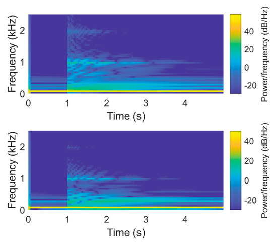
Figure 3.
Spectrogram showing the spectral content at different time instances. Trf1 was switched on at 1 s while Trf2 was still in service.
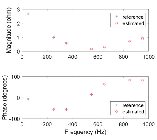
Figure 4.
The reference and the estimated impedance of the modeled distribution grid seen from the secondary side of the HV-MV transformer.
Since the modeled network was linear, there was no harmonic injection from the customers’ side. Major power electronics connected loads and sources were represented by approximated values of capacitance. Thus, the perturbation in voltage caused a linear response in terms of current. The uncertainty of the calculated impedance parameters caused by the use of a linear Norton’s equivalent model is zero. However, the real grid is a complex non-linear system. Though it can be approximated by an LTI system (Norton’s equivalent model) around the point of equilibrium, the uncertainty of this model needs to be estimated. For this purpose, a (sub-)grid of the distribution grid on the customer side of the PCC-LV (secondary side of the MV-LV transformer) was modeled in detail with additional power-electronics based non-linear loads.
4.2. Sub-Grid with Additional Non-Linear Components
A 3-phase constant current converter and three single-phase diode bridge rectifier connected loads were added at the customer side of the PCC. A capacitor bank was added to improve the power factor. The modeled customer’s side grid behind the MV-LV transformer is presented in the Figure 5. Addition of the non-linear loads lead to harmonic distortion contribution from the customer side on the PCC. Harmonic contribution from the customer side can be calculated utilizing the Norton’s equivalent model of the sub-grid. The voltage and current harmonic phasors calculated on recorded waveforms at PCC-LV during the switching of two circuit breakers (both sides of the Trf) at time t = 11 s and 21 s are shown in Figure 6. Pre- and post-event data is recorded to estimate the impedance () and current injection from the customer’s side () which are the model’s parameters.
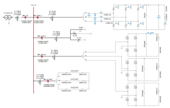
Figure 5.
Detailed model of the customer’s side grid behind the MV-LV transformer (Point of Common Coupling–PCC). Along with the linear load components, a three-phase constant current converter (LOAD_2), three single-phase diode bridge rectifier connected loads (LOAD_4) and a capacitor bank (LV_bank) are added.
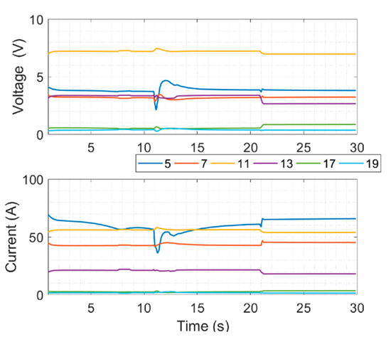
Figure 6.
Change of states observed in the voltage (top) and current (bottom) harmonic phasors calculated on simulated data measured at PCC-LV. Breaker Brk_Trf1a was switched on at 11 s while Trf2 was still in service. Breaker Brk_Trf1b was switched on at 21 s.
As the Norton’s equivalent model is linear and the system modeled is non-linear in nature, information about uncertainty in the estimated model parameters becomes more important. The two proposed uncertainty estimation methods were implemented on the PCC-LV at 0.4 kV.
5. Results
First, the customer’s side sub-grid aggregated harmonic impedance was calculated using the pre- and post-event measurements at PCC-LV. Then the two methods to estimate the uncertainty in the customer’s impedance was applied. The resulting impedance estimates and calculated harmonic current injections are presented in the Table 3. A plot of magnitude and phase of the calculated impedance and along with the reference impedance is plotted in Figure 7. It is advised in [6] that the steady state voltage and currents phasors calculated pre and post events should be utilized to estimate the impedance. For this reason, phasors calculated pre and post switching of breaker Brkr_Trf1b at time 21 s were utilized.
Table 3.
Customer side impedance and magnitude of Norton’s current injection calculated using transformer switching event at time t = 21 s.
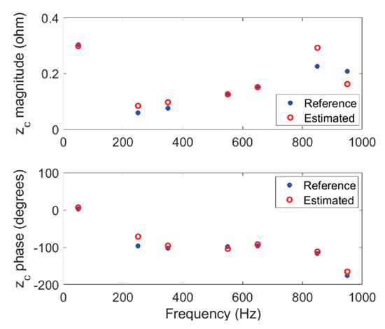
Figure 7.
The reference and the estimated impedance of the sub-grid seen from PCC-LV.
5.1. Uncertainty Calculation Using VDC Method
The harmonic voltage distortion caused by the customers at the PCC was calculated using Equations (4) and (6). Table 4 presents the calculated voltage distortions using the IEC and VHV methods for , , , , and harmonic orders.
Table 4.
Voltage distortion comparison (VDC) method: Calculated harmonic voltage distortion by the customer.
The difference in the real and imaginary parts of for each harmonic is used to fill the diagonal elements of the covariance matrix . Equation (16) is used to calculate the variance in the impedance estimates. The uncertainties in the up to 2 standard deviations were calculated and are presented in the Figure 8 using randomly generated points in the calculated uncertainty region. It can be observed that the reference impedance values fall under the uncertainty region.
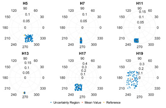
Figure 8.
Compass plot of the customer side sub-grid impedance estimates (red dots) and the uncertainty region (blue dots) calculated using the VDC method. The reference impedance values are shown using yellow dots.
5.2. Uncertainty Calculation Using CIC Method
For this method, the Norton’s current injections were calculated using the voltage and current measurements at the PCC at two separate time instances: pre and post the event. The calculated injections using values shown in the Table 3 and for the same harmonic orders are presented in the Table 5.
Table 5.
Norton’s current injection comparison (CIC) method: Customer side impedance and magnitude of Norton’s current injection calculated using transformer charging event and calculated harmonic emission by the customer.
The differences in the calculated current injections () were used fill the diagonal elements of the covariance matrix . Equation (12) was used to calculate the variance of the impedance estimates utilizing the function given by Equation (21). The uncertainties in the up to 2 standard deviations were calculated and are presented in the Figure 9 using randomly generated points in the calculated uncertainty region.
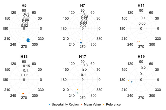
Figure 9.
Compass plot of the customer side sub-grid impedance estimates (red dots) and the uncertainty region (blue dots) calculated using Norton’s CIC method. The reference impedance values are shown using yellow dots.
It was observed that the CIC method gives a very narrow envelope of uncertainty when compared to the VDC method. However, the uncertainty range given by the VDC method envelopes the reference impedance at all frequencies. Another difference between the two methods is that the VDC method requires the knowledge of the utility impedance at the PCC. The importance of the accuracy of the known utility impedance was realized when both methods were applied to transformers-switching event data while the diode rectifier and the converter were switched off (a linear load condition). The CIC method gave zero variance. This was expected because, for a linear load, the current injection before and after the event was zero. The VDC method, however, gave a certain variance because of the difference in the harmonic emission calculated by the IEC and VHV methods caused by the error in the known utility impedance. Thus, it can be said that the VDC method gives a more conservative (broad) uncertainty range while the CIC method gives a more optimistic (narrow) uncertainty range around the estimated impedance results.
6. Discussion
The presented simulation study is an ideal case scenario with no measurement errors. In handling field data, it becomes critical to set a minimum threshold for event detection at all frequencies. The bigger the threshold the less the effect of noise errors. As shown in [10], relative change in the harmonic current phasor to the change in fundamental current phasor can be used to set a minimum threshold for an event to be considered suitable for data acquisition. The accuracy of the sensors used for data acquisition is also crucial in determining the accuracy of the estimates. However, the aim of this paper was to propose two different methods to calculate the uncertainty of the impedance estimates in presence of non-linear loads. Presence of non-linear devices makes the assumed linear property of the grid less correct and the knowledge of uncertainty of impedance parameters calculated using the incorrect linear grid model becomes important.
The (sub-)grid impedance will vary as the loads vary. One of the limitations of the measurement-based methods is that the calculated impedance using data from a single event will only give a snapshot of the grid impedance for a particular set of loading and background harmonics. Several such measurement-based snapshots may be required to get impedance results during different loading conditions of the (sub)-grid. Another drawback is that the impedance values can only be calculated up to the frequencies which are perturbed by the event. So, impedance calculations over a broad range of frequencies (especially for the higher frequencies) may not be possible for some events.
Validation of the estimated impedance parameters of Norton’s equivalent model of a physical grid is a very challenging task. Actual impedance of the (sub-)grid is unknown and the distortions in the voltage and current signals measured at the PCC are a superimposed effect of emission from the customer’s side sub-grid and the background distortion from the utility’s side grid. Therefore the proposed methods to estimate the uncertainty range of the calculated impedance values are important for generating reliable models of the grid.
7. Conclusions
This paper presented two methods to compute the uncertainty of Norton’s equivalent model’s impedance parameters in the presence of non-linear loads. The voltage distortion comparison method compares the customer emissions (voltage distortion at PCC caused by the customer’s side) calculated by the VHV and IEC methods. The IEC method uses only the utility impedance to estimate the customer’s emission whereas the VHV method utilized both utility’s and the customer’s side impedance. Given that both the methods should give similar emission values, the difference in the calculated emissions was utilized to calculate the uncertainty present in the customer impedance using the theory of error propagation. This method, however, requires the knowledge of the utility impedance at the PCC.
The current injection comparison method does not require the knowledge of the utility side impedance and compares the value of calculated harmonic injection at times before and after the event. Given that the linear Norton model’s injection should remain constant before and after the event, the difference in the injection current is used to calculate the variance in the customer’s impedance.
It was found that the VDC method gives a broader uncertainty range that is more likely to envelope the actual impedance values whereas the CIC method gives very narrow uncertainty range and, when compared to the VDC method, is less likely to envelope the actual impedance value. The given two methods could be utilized to provide additional information about the results obtained while making aggregated Norton’s equivalent models of the customer’s side of the grid. More information about the uncertainty in the grid model in presence of non-linear devices would help discard the unreliable results obtained by a measurement campaign.
Author Contributions
Conceptualization, R.S.S.; investigation, R.S.S.; methodology, R.S.S.; project administration, V.Ć.; supervision, V.Ć. and S.C.; writing—original draft, R.S.S.; writing—review and editing, R.S.S., S.C. and V.Ć. All authors have read and agreed to the published version of the manuscript.
Funding
This work has received funding from the European Union’s Horizon 2020 research and innovation programme MEAN4SG under the Marie Skłodowska-Curie grant agreement 676042.
Conflicts of Interest
The authors declare no conflict of interest. The funders had no role in the design of the study; in the collection, analyses, or interpretation of data; in the writing of the manuscript, or in the decision to publish the results.
References
- D’Antona, G.; Muscas, C.; Sulis, S. State Estimation for the Localization of Harmonic Sources in Electric Distribution Systems. IEEE Trans. Instrum. Meas. 2009, 58, 1462–1470. [Google Scholar] [CrossRef]
- Barakou, F.; Bollen, M.H.J.; Mousavi-Gargari, S.; Lennerhag, O.; Wouters, P.A.A.F.; Steennis, E.F. Impact of Load Modeling on the Harmonic Impedance Seen from the Transmission Network. In Proceedings of the 2016 17th International Conference on Harmonics and Quality of Power (ICHQP), Belo Horizonte, Brazil, 16–19 October 2016; pp. 283–288. [Google Scholar]
- Enslin, J.H.R.; Heskes, P.J.M. Harmonic Interaction between a Large Number of Distributed Power Inverters and the Distribution Network. IEEE Trans. Power Electron. 2004, 4, 1586–1593. [Google Scholar] [CrossRef]
- Cuk, V.; Cobben, J.F.G.; Kling, W.L.; Ribeiro, P.F. Considerations on Harmonic Impedance Estimation in Low Voltage Networks. In Proceedings of the 2012 IEEE 15th International Conference on Harmonics and Quality of Power, Hong Kong, China, 17–20 June 2012; pp. 358–363. [Google Scholar]
- Meyer, J.; Stiegler, R.; Schegner, P.; Röder, I.; Belger, A. Harmonic Resonances in Residential Low-Voltage Networks Caused by Consumer Electronics. CIRED Open Access Proc. J. 2017, 672–676. [Google Scholar] [CrossRef]
- Xu, W.; Ahmed, E.E.; Zhang, X.; Liu, X. Measurement of Network Harmonic Impedances: Practical Implementation Issues and Their Solutions. IEEE Trans. Power Deliv. 2002, 17, 210–216. [Google Scholar]
- Girgis, A.A.; McManis, R.B. Frequency Domain Techniques for Modeling Distribution or Transmission Networks Using Capacitor Switching Induced Transients. IEEE Trans. Power Deliv. 1989, 4, 1882–1890. [Google Scholar] [CrossRef]
- Borkowski, D.; Wetula, A.; Bień, A. New Method for Noninvasive Measurement of Utility Harmonic Impedance. In Proceedings of the 2012 IEEE Power and Energy Society General Meeting, San Diego, CA, USA, 22–26 July 2012; pp. 1–8. [Google Scholar]
- Nagpal, M.; Xu, W.; Sawada, J. Harmonic Impedance Measurement Using Three-Phase Transients. IEEE Trans. Power Deliv. 1998, 13, 272–277. [Google Scholar] [CrossRef]
- Serfontein, D.; Rens, J.; Botha, G.; Desmet, J. Continuous Event-Based Harmonic Impedance Assessment Using Online Measurements. IEEE Trans. Instrum. Meas. 2016, 65, 2214–2220. [Google Scholar] [CrossRef]
- Monteiro, H.L.; Duque, C.A.; Silva, L.R.; Meyer, J.; Stiegler, R.; Testa, A.; Ribeiro, P.F. Harmonic Impedance Measurement Based on Short Time Current Injections. Electr. Power Syst. Res. 2017, 148, 108–116. [Google Scholar] [CrossRef]
- Riccobono, A.; Liegmann, E.; Pau, M.; Ponci, F.; Monti, A. Online Parametric Identification of Power Impedances to Improve Stability and Accuracy of Power Hardware-In-The-Loop Simulations. IEEE Trans. Instrum. Meas. 2017, 66, 2247–2257. [Google Scholar] [CrossRef]
- Robert, A.; Deflandre, T.; Gunther, E.; Bergeron, R.; Emanuel, A.; Ferrante, A.; Finlay, G.S.; Gretsch, R.; Guarini, A.; Iglesias, J.L.G.; et al. Guide for Assessing the Network Harmonic Impedance. In Proceedings of the 14th International Conference and Exhibition on Electricity Distribution. Part 1. Contributions (IEE Conf. Publ. No. 438), Birmingham, UK, 2–5 June 1997; Volume 2, p. 3-1. [Google Scholar]
- Busatto, T.; Larsson, A.; Rönnberg, S.K.; Bollen, M.H.J. Including Uncertainties From Customer Connections in Calculating Low-Voltage Harmonic Impedance. IEEE Trans. Power Deliv. 2019, 34, 606–615. [Google Scholar] [CrossRef]
- Busatto, T.; Ravindran, V.; Larsson, A.; Rönnberg, S.K.; Bollen, M.H.; Meyer, J. Deviations between the Commonly-Used Model and Measurements of Harmonic Distortion in Low-Voltage Installations. Electr. Power Syst. Res. 2020, 180, 1–6. [Google Scholar] [CrossRef]
- International Electrotechnical Commission (IEC). Testing and Measurement Techniques—General Guide on Harmonics and Interharmonics Measurements and Instrumentation, for Power Supply Systems and Equipment Connected Thereto; Technical Report No. IEC 61000-4-7; International Electrotechnical Commission (IEC): Geneva, Switzerland, 2009. [Google Scholar]
- Xu, W.; Liu, Y. A Method for Determining Customer and Utility Harmonic Contributions at the Point of Common Coupling. IEEE Trans. Power Deliv. 2000, 15, 804–811. [Google Scholar]
- International Electrotechnical Commission (IEC). Electromagnetic Compatibility (EMC)—Part 3-6: Limits—Assessment of Emission Limits for the Connection of Distorting Installations to MV, HV and EHV Power Systems; Technical Report No. IEC TR 61000-3-6; International Electrotechnical Commission (IEC): Geneva, Switzerland, 2008. [Google Scholar]
- Špelko, A.; Blažič, B.; Papič, I.; Pourarab, M.; Meyer, J.; Xu, X.; Djokic, S.Z. CIGRE/CIRED JWG C4.42: Overview of Common Methods for Assessment of Harmonic Contribution from Customer Installation. In Proceedings of the 2017 IEEE Manchester PowerTech, Manchester, UK, 18–22 June 2017; pp. 1–6. [Google Scholar]
- Papič, I.; Matvoz, D.; Špelko, A.; Xu, W.; Wang, Y.; Mueller, D.; Miller, C.; Ribeiro, P.F.; Langella, R.; Testa, A. A Benchmark Test System to Evaluate Methods of Harmonic Contribution Determination. IEEE Trans. Power Deliv. 2019, 34, 23–31. [Google Scholar] [CrossRef]
- Evaluation of Measurement Data—Supplement 2 to the “Guide to the Expression of Uncertainty in Measurement. Available online: https://www.bipm.org/utils/common/documents/jcgm/JCGM_102_2011_E.pdf (accessed on 25 April 2017).
- Hall, B.D. On the Propagation of Uncertainty in Complex-Valued Quantities. Metrol. 2004, 41, 173–177. [Google Scholar] [CrossRef]
- Ribeiro, P.F. Guidelines on Distribution System and Load Representation for Harmonic Studies. In Proceedings of the ICHPS V International Conference on Harmonics in Power Systems, Atlanta, GA, USA, 22–25 September 1992; pp. 272–280. [Google Scholar] [CrossRef]
- Burch, R.; Chang, G.; Hatziadoniu, C.; Grady, M.; Liu, Y.; Marz, M.; Ortmeyer, T.; Ranade, S.; Ribeiro, P.; Xu, W. Impact of Aggregate Linear Load Modeling on Harmonic Analysis: A Comparison of Common Practice and Analytical Models. IEEE Trans. Power Deliv. 2003, 18, 625–630. [Google Scholar] [CrossRef]
- Ye, G.; Sans, A.; Cuk, V.; van Waes, J.; Cobben, S. Impact of Distribution Network Modelling on Harmonic Impedance in the HV Grid. In Proceedings of the CIRED 2019 Conference, Madrid, Spain, 3–6 June 2019. [Google Scholar]
- Bhattacharyya, S.; Wang, Z.; Cobben, J.F.G.; Myrzik, J.M.A.; Kling, W.L. Analysis of Power Quality Performance of the Dutch Medium and Low Voltage Grids. In Proceedings of the 2008 13th International Conference on Harmonics and Quality of Power, Wollongong, NSW, Australia, 28 September–1 October 2008; pp. 1–6. [Google Scholar]
- Gole, A.; Irwin, G.; Nayak, O.; Woodford, D. EMTDC User’s Guide; Fifth Printing; Manitoba Hydro International, Ltd.: Winnipeg, MB, Canada, 2010. [Google Scholar]
- Serfontein, D.; Rens, J.; Botha, G.; Desmet, J. Improved Event Based Method for Harmonic Impedance Assessment. In Proceedings of the 2016 IEEE International Workshop on Applied Measurements for Power Systems (AMPS), Aachen, Germany, 28–30 September 2016; pp. 1–6. [Google Scholar]
- Peng, J.; Li, H.; Wang, Z.; Ghassemi, F.; Jarman, P. Influence of Sympathetic Inrush on Voltage Dips Caused by Transformer Energisation. IET Gener. Transm. Distrib. 2013, 7, 1173–1184. [Google Scholar] [CrossRef]
- Welch, P. The Use of Fast Fourier Transform for the Estimation of Power Spectra: A Method Based on Time Averaging over Short, Modified Periodograms. IEEE Trans. Audio Electroacoust. 1967, 15, 70–73. [Google Scholar] [CrossRef]


© 2020 by the authors. Licensee MDPI, Basel, Switzerland. This article is an open access article distributed under the terms and conditions of the Creative Commons Attribution (CC BY) license (http://creativecommons.org/licenses/by/4.0/).