1. Introduction
Due to the advantages of two-level voltage source inverters, they have received more and more attention in the field of renewable energy generation systems, including photovoltaic systems and energy storage systems, among others. Recently, the control methods of two-level voltage source inverters have been widely studied to achieve smooth and flexible energy conversion [
1,
2,
3,
4,
5]. As is known, vector control is widely used to control two-level voltage source inverters in renewable energy generation systems as it can achieve power decoupling control. Nevertheless, proportional and integral controller and pulse width modulation modules are needed, which makes the control system hard to debug and prolongs the development cycle of the control system. Another control method, i.e., direct power control, has also been studied to control two-level voltage source inverters. Compared to vector control, proportional and integral controller and pulse width modulation modules are removed. However, as the switching frequency is unfixed and the optimal voltage vector is selected based on an offline switch table, its power control precision is relatively low.
As a simple but effective control method, model predictive control (MPC) has received much more attention in the field of the optimal control of two-level voltage source inverters lately.
An MPC strategy was designed to control the current of two-level voltage source inverters in [
6] in 2007. From then on, many researchers began to study new MPC strategies to reduce the computational time [
7,
8], to lower the switching frequency [
9,
10], to suppress the common-mode voltage [
11,
12], to decrease the current ripples [
13,
14,
15,
16,
17,
18,
19,
20,
21,
22,
23,
24,
25,
26,
27,
28,
29], or to minimize the power ripples [
30,
31,
32].
In [
7,
8], according to the deadbeat control principle, voltage-based cost functions are designed to replace the conventional current-based cost function. Thus, the calculation burden is reduced significantly. In [
9,
10], the concept of multistep MPC is studied and evaluated, which can reduce the switching frequency obviously, making it very suitable for large power converters. In [
11,
12], common-mode voltage suppression methods are studied using an MPC strategy. Thus, the negative effects of the common-mode voltage are reduced.
Additionally, as a flexible control method, MPC strategies are also studied in [
13,
14,
15,
16,
17,
18,
19,
20,
21,
22,
23,
24,
25,
26,
27,
28,
29] to reduce the current ripples by using more voltage vectors instead of only one in every control cycle. In [
13,
14,
15], dual-vector MPC strategies are studied. Compared to the conventional single-vector MPC, the control precision is improved as more voltage vectors are utilized in every control cycle. Moreover, in [
16,
17,
18,
19,
20,
21], three voltage vectors are chosen per control cycle to further enhance the control performance, and better results are obtained. In these methods in [
13,
14,
15,
16,
17,
18,
19,
20,
21], the duty cycles of each voltage vector are figured out according to the deadbeat control theory. Although duty cycles can be calculated accurately theoretically, the actual calculated duty cycle may be smaller than zero or larger than one, which reduces the control performance to a certain extent.
Alternately, there is another way to determine the duty cycles, which is named modulated MPC [
22,
23,
24,
25,
26,
27,
28,
29]. In this type of method, the duty cycle of each voltage vector is deduced by assuming that it is inversely proportional to its cost function value. As it is simple but effective, many researchers have studied modulated MPC to control the cascaded H-bridge converter [
22], the multilevel solid-state transformer [
23], the direct and indirect matrix converter [
24,
25], the shunt active filter [
26], the brushless doubly fed induction machine [
27], the two-level three-phase inverter [
28,
29], and so on. However, although it is shown in [
22,
23,
24,
25,
26,
27,
28,
29] that the modulated MPC method can achieve current control, up to now, there still lacks a solid theoretical support for this kind of method, which hinders its popularization and application.
Additionally, to minimize the power ripples of the converters, modified MPC strategies have also been studied in [
26,
30,
31,
32]. However, there are still few papers to study the optimal modulated model predictive direct power control methods as well as the theoretical analysis for power converters.
To fill this gap, a novelty dual-vector modulated MPC strategy is presented for two-level voltage source inverters with a new duty cycle calculation method as well as a detailed theoretical analysis. First, twelve hybrid voltage vectors are constructed according to the eight basic voltage vectors of the two-level voltage source inverter. Next, to decrease the computation amount, the reference voltage is deduced based on the reference current, and a cost function based on the voltage error is designed. Then, only three hybrid voltage vectors are required to be evaluated online per control period based on the information of the reference voltage. Finally, the optimal voltage vector combination is selected.
The main contributions of this paper lie in three aspects.
The first one is that a new duty cycle calculation method of each voltage vector is proposed in this paper according to the hypothesis that it is inversely proportional to the square root of its cost function value.
The next one is that, based on a detailed theoretical analysis, the validity of the presented dual-vector modulated MPC strategy with the new duty cycle calculation method is proved based on the geometrical relationship of the voltage vectors, which is also verified by experimental results.
The third one is that the proposed dual-vector modulated MPC strategy can also be applied to control other types of inverters, such as three-phase four-switch inverters, whose effectiveness is also proved by the geometrical relationship of the voltage vectors as well as the experimental results.
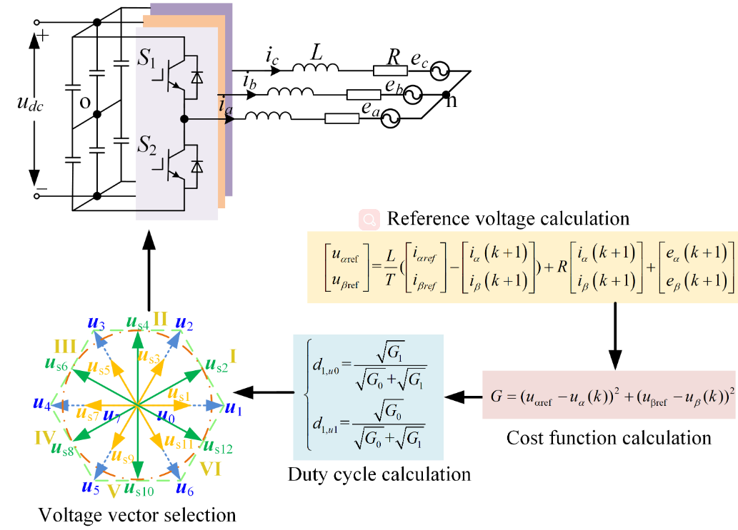
2. Conventional MPC Strategy
Figure 1 depicts the topology of two-level voltage source inverters. As is known, there are eight voltage vectors for two-level voltage source inverters, including
u0(000),
u1(100),
u2(110),
u3(010),
u4(011),
u5(001),
u6(101), and
u7(111), which are shown in
Figure 2.
Typically, (1) shows the mathematical equation of two-level voltage source inverters on the
α-
β reference.
where
uα, uβ and
iα,
iβ are the output AC voltages and currents, respectively, and
eα and
eβ are the back electromotive forces (EMFs).
L stands for the filter inductance with
R denoting the parasitic resistance on it.
If the sample and control cycle is
T, based on the Euler’s discretization formula, it can be calculated that
Based on (2), as well as the sampled current
iα(
k) and
iβ(
k) at the
kth instant, the current
iα(
k + 1) and
iβ(
k + 1) at the next control cycle can be calculated, as depicted in (3).
As there is an inherent one-step delay in the MPC system, to reduce its influences, it can be compensated by using the optimal voltage vector selected in the last control period to predict the current
iα(
k + 1) and
iβ(
k + 1) firstly. Next, the eight basic voltage vectors
uk+1 = [
uα(
k + 1),
uβ(
k + 1)]
T can be further utilized to calculate the current
iα(
k + 2) and
iβ(
k + 2) based on (4).
Finally, by evaluating the prediction errors of all the eight basic voltage vectors using the cost function defined in (5), an optimal voltage vector can be chosen and utilized to control the inverter during the next control cycle.
where
iαref and
iβref are the reference currents.
As only one voltage vector is utilized in every control cycle in the above conventional MPC strategy, the current total harmonic distortion (THD) is quite large.
Aiming to solve this problem, a dual-vector modulated MPC strategy is presented in this paper by using two voltage vectors in every control cycle. Detailed theoretical analysis is carried out to verify the validity of the presented dual-vector modulated MPC strategy. Comparative experimental results also verified its effectiveness.
3. Dual-Vector Modulated MPC Strategy
According to [
7,
8], to simplify the MPC strategy, a cost function based on the reference voltage is defined in this paper.
First, the reference voltage is deduced according to the deadbeat control theory, which is shown in (6).
where
uαref and
uβref are the reference voltages.
To limit the voltage within the linear modulation region, if
,
uαref and
uβref are calculated based on (7).
Then, a voltage-based cost function is defined as
Through using this voltage-based cost function, the calculation burden can be reduced as the prediction of the current for many times in each control cycle is not required any more.
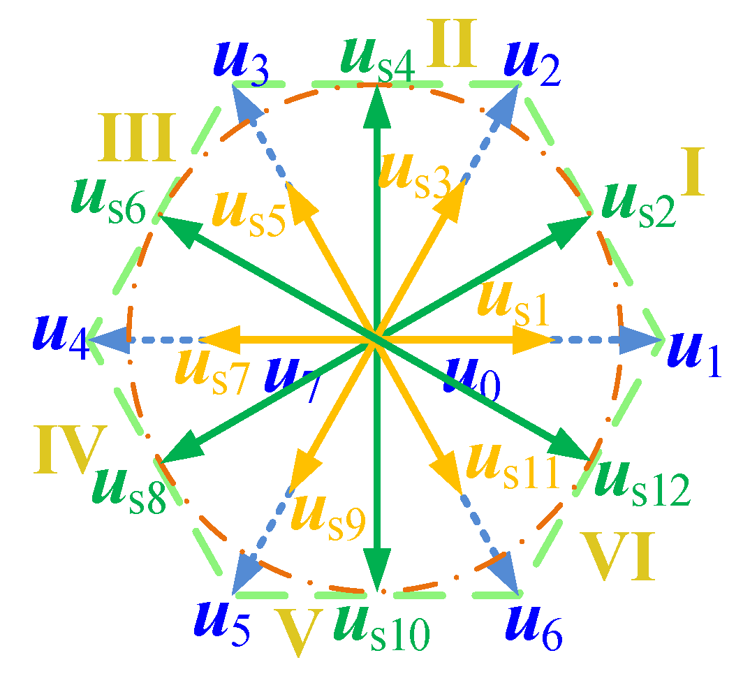
To select and apply two voltage vectors per control period, twelve hybrid voltage vectors are constructed according to the eight basic voltage vectors of the two-level voltage source inverter. They are
us1(
u0,
u1),
us2(
u1,
u2),
us3(
u7,
u2),
us4(
u2,
u3),
us5(
u0,
u3),
us6(
u3,
u4),
us7(
u7,
u4),
us8(
u4,
u5),
us9(
u0,
u5),
us10(
u5,
u6),
us11(
u7,
u6), and
us12(
u6,
u1), respectively, which are illustrated in
Figure 3.
The relationship between the twelve constructed hybrid voltage vectors and the basic voltage vectors is depicted in (9).
where
di,uj +
di,uk = 1,
di,uj is the duty cycle of
uj and
di,uk is the duty cycle of
uk.
For example, as
us1 is combined by
u0 and
u1, their relationship can be expressed as
To calculate the values of the twelve constructed hybrid voltage vectors, the duty cycles of the basic voltage vectors should be calculated first. Different from the methods in [
22,
23,
24,
25,
26,
27,
28,
29], which lack theoretical support, here a new duty cycle calculation method is proposed by assuming that it is inversely proportional to the square root of its cost function value, as shown in (11), where
m is a positive coefficient. In
Section 4, the effectiveness of this proposed hypothesis is verified in detail by a particular theoretical analysis.
Based on (9) and (11), the duty cycles of the basic voltage vectors are deduced. For instance, the duty cycles of
u0 and
u1 that construct
us1 can be calculated based on (12).
where
G0 and
G1 are the values of the cost function shown in (8), which are obtained by substituting
u0 and
u1 into (8), respectively.
Finally, based on (9)–(12), the combined voltage vectors are figured out.
To simplify the predictive control, the voltage vector plane can be divided into six sectors, as illustrated in
Figure 3. Then, according to the reference voltage shown in (6) and (7), its location can be obtained easily based on
Table 1, where
θ = arctan(
uβref/
uαref).
Based on the position of the reference voltage, the alternative voltage vectors that should be evaluated online can be preselected based on
Table 2. For instance, if the reference voltage is located at sector I, only
us1,
us2, and
us3 require to be evaluated online. So, as only three instead of twelve voltage vectors are required to be evaluated online, the calculation amount is reduced notably. Then, an optimal hybrid voltage vector among the three hybrid voltage vectors can be chosen to control the inverter in the next control cycle.
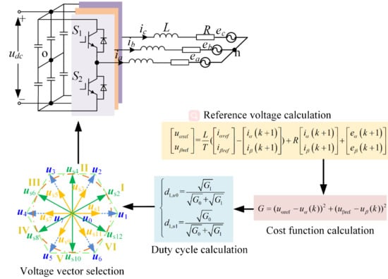
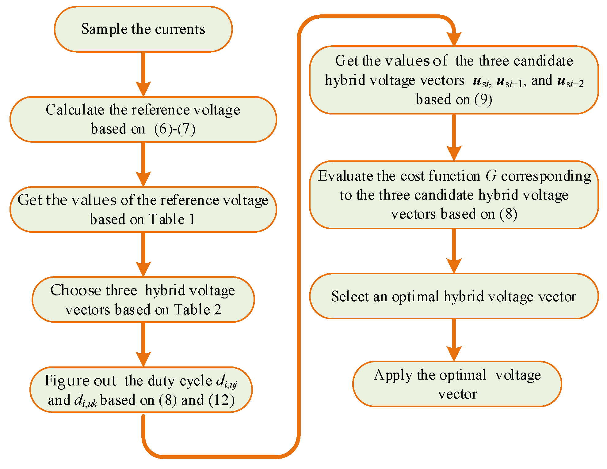
For clarity,
Figure 4 is given to show the control principle of the presented strategy. Moreover, the detailed implementation steps are also depicted below.
Step 1: Calculate the reference voltage based on (6) and (7);
Step 2: Get the values of the reference voltage based on
Table 1;
Step 3: Choose three candidate voltage vectors based on
Table 2;
Step 4: Figure out the duty cycles of the basic voltage vectors that construct the three candidate voltage vectors based on (8) and (12);
Step 5: Get the values of the three candidate voltage vectors based on (9);
Step 6: Evaluate the cost function values of the three candidate voltage vectors based on (8) and select the voltage vector that can minimize the cost function as the optimal one.
Finally, the optimal vector is utilized to control the voltage source inverter.
4. Theoretical Analysis of the Proposed Method
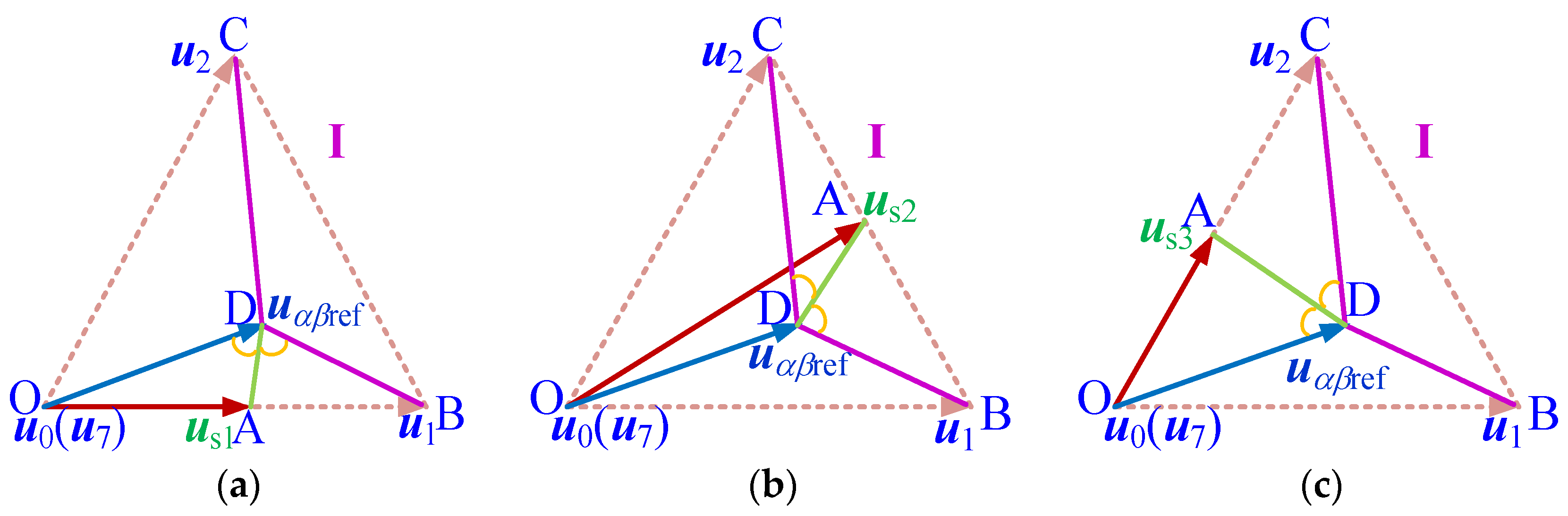
To validate the correctness of the presented duty cycle calculation method shown in (11), a rigorous theoretical analysis is proposed. Here, the case that the reference voltage vector is located at sector I is taken as an example, where it overlaps with the segment OD in
Figure 5.
As
us1 is constructed by
u0 and
u1, their relationship has been shown in (10). Based on (10), (13) can be deduced.
Based on (13) and
Figure 5(a), it can be known that |OA| =
d1,u1*|
u1 −
u0| and |AB| =
d1,u0*|
u1 −
u0|. Thus, |OA|/|AB| =
d1,u1/
d1,u0. According to (11) and (12), it can be deduced that
According to the cost function shown in (8), it can be known that
Thus, it can be deduced that
By rearranging (16) with the law of sines in consideration, it can be further deduced that
Considering that ∠OAD + ∠DAB = π, it can be known that
Thus, (19) is finally deduced based on (17) and (18).
Based on (19), it can be calculated that ∠ODA + ∠ADB = π or ∠ODA = ∠ADB. In the following, both of the two cases are analyzed respectively.
First, if ∠ODA + ∠ADB = π is true, it can be calculated that point D must be located on the segment OB. In this situation, it can be figured out based on (16) that point D and point A will be the same point. That means us1 = uαβref is true. Thus, the current control error can be minimized under this condition, which shows the validity of the duty cycle calculation algorithm proposed in this article.
Second, if point D is not located on the segment OB, ∠ODA = ∠ADB should be true. In this situation, it can be obtained that ∠ODA = ∠ADB < ∠OAD as ∠OAD = ∠ADB + ∠DBA. As ∠DOA < π/3 is true, and ∠ODA + ∠OAD + ∠DOA = π, it can be deduced that ∠ODA + ∠OAD >2π/3. As ∠OAD is larger than ∠ODA, ∠OAD > π/3 > ∠ODA can be deduced. As ∠DOA < π/3 and ∠OAD > π/3 are true, it can be known that ∠OAD > ∠DOA. According to the law of sines, |OD| > |AD| is finally deduced. As |AD| stands for the square root value of the cost function of us1, and |OD| denotes the square root value of the cost function of u0, a conclusion is obtained, i.e., the control accuracy is increased when us1 is utilized to replace u0.
Similarly, it is easy to verify that |DB| > |AD| is true, which means the control accuracy of
us1 is increased compared to that of
u1. Moreover, based on
Figure 5b,c, it can also be verified that the control error can be reduced by using
us2 or
us3 instead of
u0,
u1, and
u2. This shows the validity of the proposed duty cycle calculation method in this work.
When the reference voltage vector locates at other sectors, similar results can be obtained. Therefore, the validity of the presented strategy is verified in terms of theory, which provides a solid foundation for its popularization and application.
6. Extensions
Although the proposed dual-vector modulated MPC is aiming to control two-level voltage source inverters, further studies in this paper show that it can also be used to control other types of inverters by only changing the voltage vectors according to the corresponding inverter, which is another important contribution of this paper.
Here, a three-phase four-switch inverter is taken as an instance to show the correctness of the presented dual-vector modulated MPC.
Figure 14 shows the topology of the three-phase four-switch inverter. The four basic voltage vectors, i.e.,
V1,
V2,
V3, and
V4, can be depicted as
Figure 15, provided that the DC voltages are well balanced as many papers have studied the DC voltage balance control methods for three-phase four-switch inverters [
33,
34,
35,
36].
To reduce the current ripples, four hybrid voltage vectors are designed in the same way with (9), as shown in
Figure 15, which are
Vs1(
V1,
V2),
Vs2(
V2,
V3),
Vs3(
V3,
V4), and
Vs4(
V4,
V1). In every control cycle, one of the four hybrid voltage vectors will be selected and utilized to reduce the current ripples.
The duty cycle of each voltage vector is calculated using the same method as (11). Then, after the four hybrid voltage vectors are determined, they are substituted into (8) to get an optimal one, which will then be utilized to control the three-phase four-switch inverter. The detailed implementation steps are similar to
Figure 4. Furthermore, theoretical analysis and experimental studies are carried out to show its correctness and superiority.
6.1. Theoretical Analysis of the Proposed Method
For convenience, the voltage vector plane is divided into four sectors, as depicted in
Figure 15. Here, the case that the reference voltage vector is located at sector I is taken as an example, as shown in
Figure 16.
First, it is assumed that the end point of
Vs1 is D, as shown in
Figure 16.
Based on (9), (20) can be deduced.
Thus, based on the geometrical relationship shown in
Figure 16, (21) is deduced.
Meanwhile, according to the duty cycle calculation method in (11), it can be deduced that
According the defined cost function in (8), it can be known that
Thus, based on (22), it is calculated that
By rearranging (24) with the law of sines in consideration, (25) is obtained.
Considering that ∠BDC + ∠ADC = π, it can be known that
Thus, (27) is finally deduced based on (25) and (26).
Based on (27), it can be calculated that ∠BCD + ∠ACD = π or ∠BCD = ∠ACD. In the following, both of the two cases are analyzed respectively.
First, if ∠BCD + ∠ACD = π is true, it can be calculated that point C must be located on the segment AB. In this situation, it can be figured out based on (24) that point C and point D will be the same point. That means Vs1= uαβref is true. Thus, the current control error can be minimized under this condition, which shows the validity of the duty cycle calculation method proposed in this article.
Second, if point C is not located on the segment AB, ∠BCD = ∠ACD should be true. In this situation, it can be obtained that ∠BCD = ∠ACD < ∠ADC as ∠ADC = ∠BCD +∠CBD. As ∠CAD < π/3 is true, and ∠CAD + ∠ADC + ∠ACD = π, it is obtained that ∠ADC + ∠ACD > 2π/3. As ∠ADC is larger than ∠ACD, ∠ADC > π/3 > ∠ACD can be obtained. As ∠CAD < π/3 and ∠ADC > π/3 are true, it can be known that ∠ADC > ∠CAD. Based on the law of sines, |AC| > |CD| is finally deduced. Since |AC| stands for the square root value of the cost function of V1, and |CD| denotes that of Vs1, a conclusion is obtained, i.e., the control accuracy is increased when Vs1 is utilized to replace V1.
Similarly, |BC| > |CD| can be proved, which means the control accuracy of Vs1 is increased compared to that of V2. Thus, a conclusion is obtained, i.e., the proposed method is still effective when it is used to control the three-phase four-switch inverter. That is to say that the proposed method can be extended.
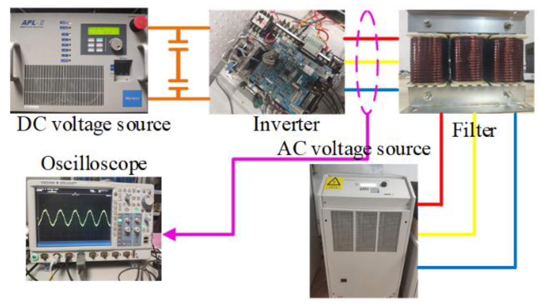
6.2. Experimental Verification
To validate the validity of the presented algorithm and the theoretical analysis shown above, experimental research is conducted, too. The parameters are the same as
Table 3.
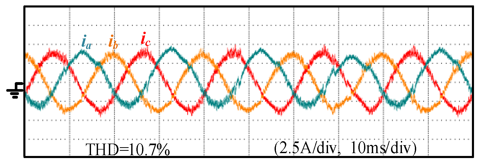
Figure 17 shows the current waveforms of the conventional single-vector MPC when the current is 4 A, while
Figure 18 is the current waveforms of the proposed dual-vector modulated MPC under the same conditions.
It is clear to see from
Figure 17 and
Figure 18 that when the proposed dual-vector modulated MPC method is utilized instead of the conventional single-vector MPC method, the current THD is decreased by 51.3%, which verifies the correctness of the presented strategy and the theoretical analysis again.
Additionally, compared to the conventional deadbeat control theory-based dual-vector MPC method [
13,
14,
15,
16,
17,
18,
19,
20,
21], the proposed method in this paper can reduce the computational time, mainly because the duty cycle calculation method of this paper is simpler with reduced mathematical operation than that of the conventional dual-vector MPC method [
13,
14,
15,
16,
17,
18,
19,
20,
21]. Thus, less digital processing time is required. Furthermore, by using the proposed voltage-based cost function as well as the proposed voltage vector selection method in this paper, the computational time of the proposed method can be further reduced.
7. Conclusions
In this paper, a dual-vector modulated MPC is proposed based on the hypothesis that the duty cycle of each voltage vector is inversely proportional to the square root of its corresponding cost function value for two-level voltage source inverters. Theoretical analysis is conducted based on the geometrical relationship of the voltage vectors for the first time to prove the correctness of the presented method. Furthermore, comparative experimental results show the superiority of the presented modulated MPC strategy, too. Moreover, at the end of the paper, the proposed dual-vector modulated MPC is extended to control the three-phase four-switch inverter. Both the theoretical analysis and the experimental results verify its effectiveness. This is another important contribution of this paper.
In the future, the proposed method should be further studied to control many other kinds of inverters, including multilevel inverters and matrix inverters, as they have similar voltage vector planes, and research should also be done to analyze its effectiveness in a similar way.
Nevertheless, the proposed method also has a few disadvantages, one of which being that although it can reduce the current ripples and THDs compared to the single-vector MPC, it cannot minimize the current ripples and THDs at all operation regions. Although the theoretical analysis shows that the proposed method can reduce the control error at all operation regions and minimize it in several special operation regions, no evidence shows that it can minimize the control error at all operation regions. Therefore, to further solve the disadvantages of the proposed method shown above and improve its control performance, much work should be done in the future to minimize the control error of the proposed method at all operation regions.


