Dynamic Modeling of Multiple Microgrid Clusters Using Regional Demand Response Programs

Abstract

Preserving the frequency stability of multiple microgrid clusters is a serious challenge. This work presents a dynamic model of multiple microgrid clusters with different types of distributed energy resources (DERs) and energy storage systems (ESSs) that was used to examine the load frequency control (LFC) of microgrids. The classical proportional integral derivative (PID) controllers were designed to tune the frequency of microgrids. Furthermore, an imperialist competitive algorithm (ICA) was proposed to investigate the frequency deviations of microgrids by considering renewable energy resources (RERs) and their load uncertainties. The simulation results confirmed the performance of the optimized PID controllers under different disturbances. Furthermore, the frequency control of the microgrids was evaluated by applying regional demand response programs (RDRPs). The simulation results showed that applying the RDRPs caused the damping of frequency fluctuations.

1. Introduction

Recently, air pollution produced by fossil fuel power plants has been causing serious environmental problems [1]. Due to environmental concerns, the tendency toward using renewable energy resources (RERs) for power generation is increasing [2]. Generally, RERs increase the reliability of the system, improve the voltage profile, and decrease the dependence on fossil fuel [3,4,5,6]. By increasing the influence of RERs, an imbalance between generation and demand occurs in power systems because of the stochastic nature of these resources [7]. To overcome this problem, the use of energy storage systems (ESSs) can be a proper solution. ESSs can inject or store energy in power systems when it is required. Furthermore, they improve the reliability, stability, and power quality of the systems [8]. The RERs have a small capacity. Therefore, they are linked to the grid at the distribution level. A distribution system that has small-scale energy resources is called a microgrid, which is also composed of loads, distributed energy resources (DERs), ESSs, and other infrastructure [9]. Generally, microgrids connect to the main grid. However, situations such as errors, voltage fluctuations, and high oscillations of the main grid are causing them to separate from the main grid and they act in isolation [10]. During the isolated operation of the main grid, the controllable power resources respond to power and load disturbances by injecting or absorbing power. Furthermore, they adjust the frequency and power of the microgrid. Due to the inherent delay and the generation rate constant (GRC) of power resources, the control instructions applied to the power resources cannot be implemented immediately. As such, frequency fluctuations will occur in the microgrids and the proper adjustment of control parameters can help the damping of frequency oscillations [11,12]. Since the power resources are operating in parallel, to acquire a stable feedback loop, it is necessary to get the speed-droop characteristic (f-P) for the power resources to participate in the frequency control.

In addition, for the power-sharing between resources, it is necessary to obtain the reverse relation of frequency droop coefficient (R) by considering the nominal value of that power resource [13,14]. Similarly, each power resource has a control signal for adjusting the output power in a manner that is proportional to the frequency oscillations, which is called frequency bias (β). Nowadays, many papers have presented the dynamic modeling of islanded microgrids [15,16,17,18,19,20]. In Abazari et al. [16], a new load frequency control (LFC) model for an independent hybrid microgrid with RERs was presented and the dynamic models for the resources were introduced. In addition, their participation in frequency control studies was considered. In A-Hamed et al. [18], the performance of a microgrid in the presence of a new control method was evaluated. The proposed microgrid had various power generation resources, including photovoltaic, wind, diesel generator, fuel cell and electrolyzer, and battery resources. A model for the microgrid was implemented through Matlab/Simulink software and the integral proportional (PI) control scheme was implemented. In Fini and Golshan [20], a microgrid with controllable and uncontrollable resources was considered. The stability of the microgrid frequency was investigated by considering the virtual inertia of the ultracapacitor unit.

Due to the position of microgrids in the development of future energy substrates, maintaining the security of microgrid electrification, especially in critical situations, is a serious challenge. One way to maintain the security of microgrid electrification is by connecting microgrids. The multiple microgrid clusters are supporting each other and increasing the reliability of the whole system [21]. In Toro and M-Nava [22], a frequency control strategy for multiple microgrid clusters that are connected by a tie-line was suggested. When load disturbances occur, the proportional integral derivative (PID) controllers are used to control the system frequency. On the other hand, the uncertainties in the generation of RERs make the PID controllers unable to perform the frequency control operation. Therefore, the use of intelligent techniques, such as a genetic algorithm and the imperialist competitive algorithm (ICA), to adjust the optimal parameters are suggested in References [23,24]. One of the factors used to engender instability is by increasing the over-frequency in power systems. Increasing the over-frequency is damaging to system equipment and it can cause outages. Therefore, demand response programs can avoid these issues and enhance power systems security [25]. References [26,27] showed that demand response programs could play an important role in the frequency regulation of the power system. In Moghadam et al. [28], an algorithm of distributed frequency control was studied through randomizing the frequency response of smart appliances. In this method, the controllers of the generation side are deactivated and the demand response is activated.

The participation of demand response programs in the frequency control of isolated microgrids and power systems was investigated in References [29,30]. In Huang and Li [31], the effect of controllable loads on the frequency response of the system and load damping coefficient was examined. In Malik and Ravishankar [32], domestic loads were considered as a source of demand response during frequency control. In Soares et al. [33], the use of demand response programs to integrate the RERs and reduce the effects of changes in the generation of these resources on power systems was proposed. In C-Chien et al. [34], the collaboration of a spinning reserve and demand response programs in frequency restoration during contingencies of the system was suggested.

Despite the high participation of demand response programs in frequency adjustments, many operating concerns remain. On the one hand, overload shedding can cause unnecessary load shedding and consequently lead the system to excessive over-frequency. On the other hand, the light usage of demand response programs during system faults may reduce the positive impact of such a method. Therefore, knowing the location of the load shedding and the exact magnitude of the disturbances, particularly in multiple microgrids, is necessary [35,36]. In Bayat et al. [37], a method was presented that used the changes of reactive power in buses to locate the changes of the active power consumption in controllable loads. In Gao and Ning [38], the wavelet analysis method was used to assess the location and size of the disturbances. In Babahajiani et al. [39], a method for determining the location of load disturbances and the magnitude of disturbances in interconnected power systems was suggested., By monitoring the power flows of the tie-lines, the proposed method determines the magnitude of disturbance and the region that disturbance occurs in and applies the response to the demand program for the affected region.

In light of the aforementioned literature, the contributions of this work can be explained as follows:

• The absence of a suitable dynamic model is one of the serious challenges for a study on LFC in multiple microgrid clusters, which restricts research activities in this field. Modeling can be done for a variety of goals. Thus, using a suitable model for a specific study goal is the preferred option. The present paper provides a suitable dynamic model for multiple microgrid clusters based on tie-lines for studying the frequency and tie-line power control.
• In this study, the Monte Carlo simulation was used to generate scenarios regarding the uncertainties of RERs and loads by considering probability distribution functions when modeling them. However, due to the uncertainties in RERs and loads, the conventional controllers, such as PID controllers, will not be suitable for LFC. Hence, adjusting the control parameters was suggested by using the ICA to solve this problem.
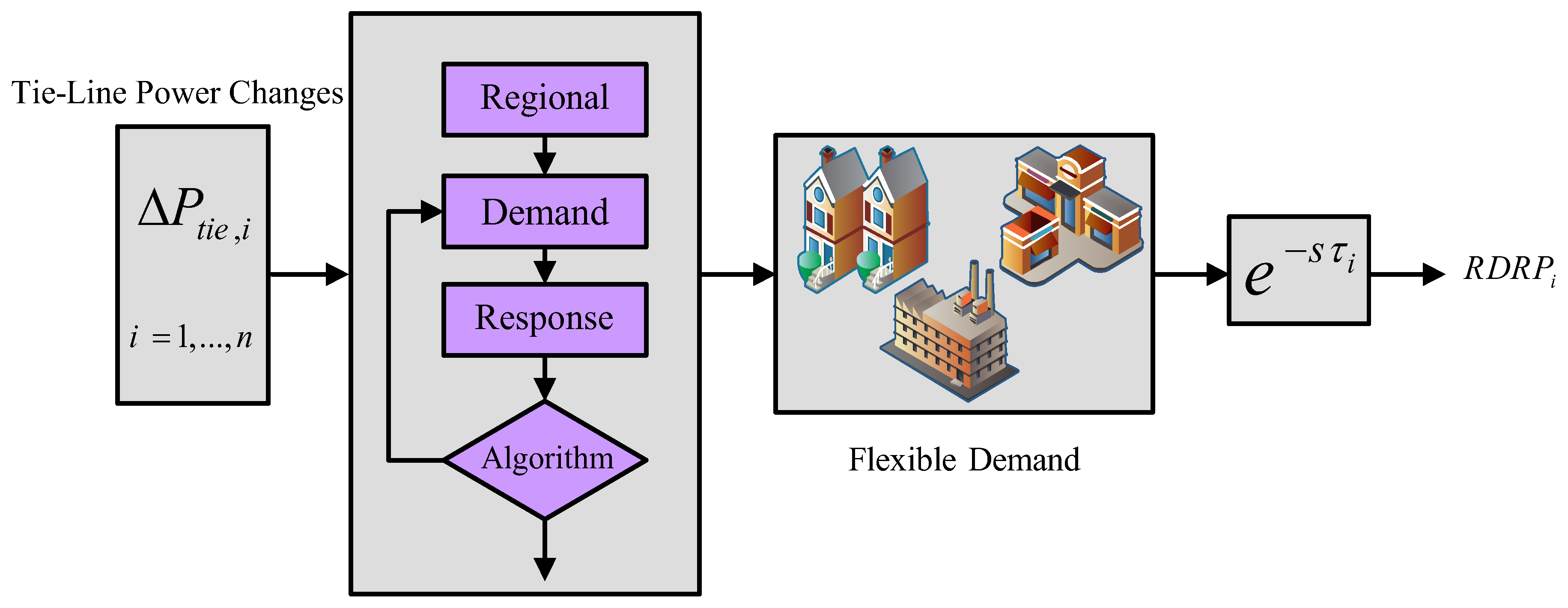
• Damping frequency fluctuations is one of the main issues of frequency control in power systems and microgrids. Due to its fast dynamics, the demand response program could be an attractive suggestion for damping system frequency fluctuations. Opposed to the other works, the regional demand response program is simpler and more accurate, and does not require complex and massive computational calculations. Furthermore, this method is applicable to almost all types of loads by considering the load’s participation coefficient in each region during the frequency control. Therefore, the regional demand response was applied for each microgrid in this study to reduce the frequency oscillations.

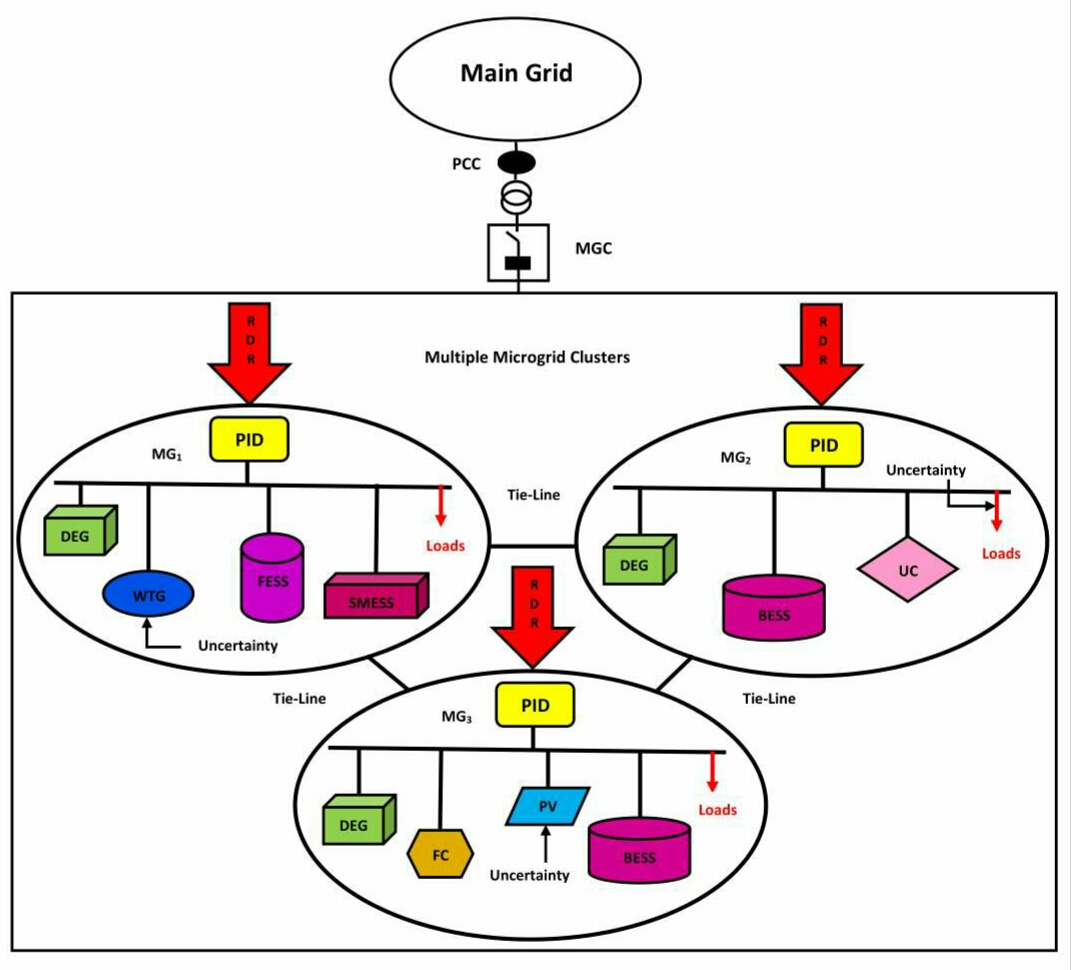
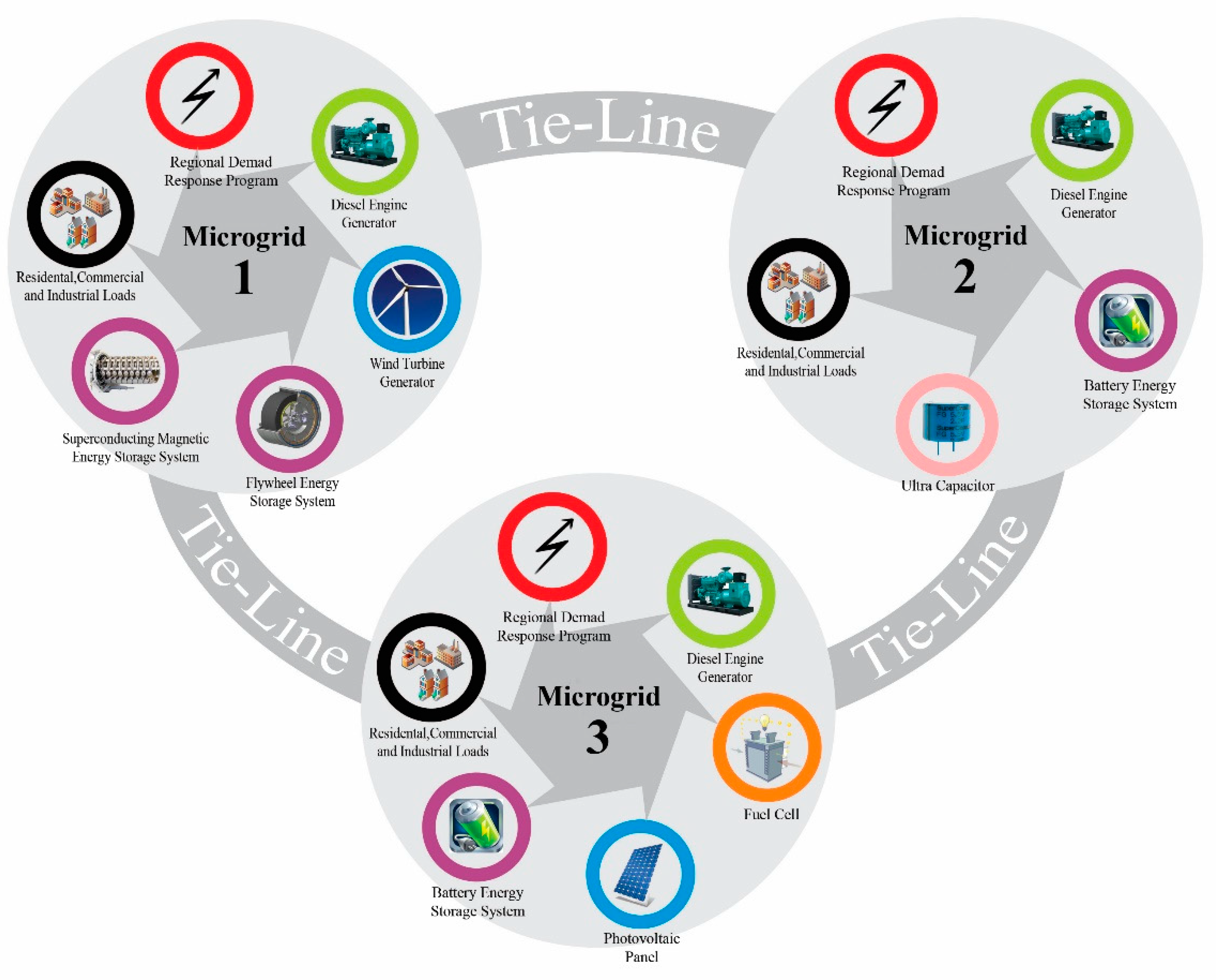
The rest of this paper is organized as follows. Section 2 presents the case study. In Section 3, the modeling of the units is explained. In Section 4, the modeling of the microgrids is depicted. Section 5 presents the modeling of multiple microgrid clusters. The modeling of uncertainties is explained in Section 6. In Section 7, the modeling of regional demand response programs is discussed. The simulation results and discussions are provided in Section 8. Finally, conclusions are given in Section 9.

2. Case Study

Here, the multiple microgrid clusters, which are isolated from the main grid and are considered for this case study, are presented. The studied multiple microgrid clusters are shown in Figure 1. In this study, three microgrids with different specifications were connected to each other using a tie-line. The first microgrid consisted of a diesel engine generator, a wind turbine generator, a flywheel energy storage system, and a superconducting magnetic energy storage system. The second microgrid included a diesel engine generator, a battery energy storage system, and an ultracapacitor. The third microgrid consisted of a diesel engine generator, a fuel cell, a photovoltaic panel, and a battery energy storage system. In addition, the RERs and load uncertainties were considered in this case study. Furthermore, the regional demand response programs (RDRPs) were applied for each microgrid.

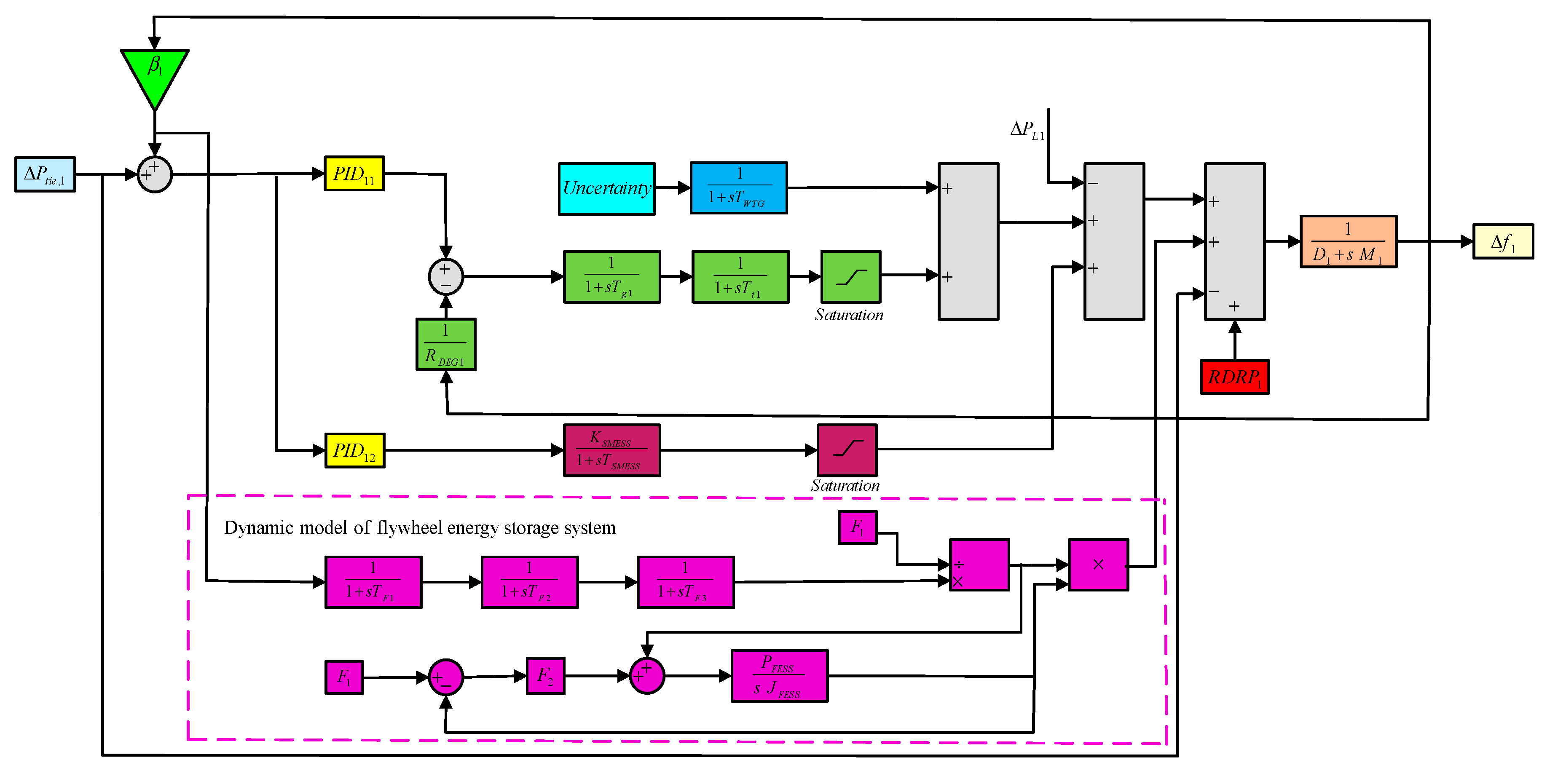
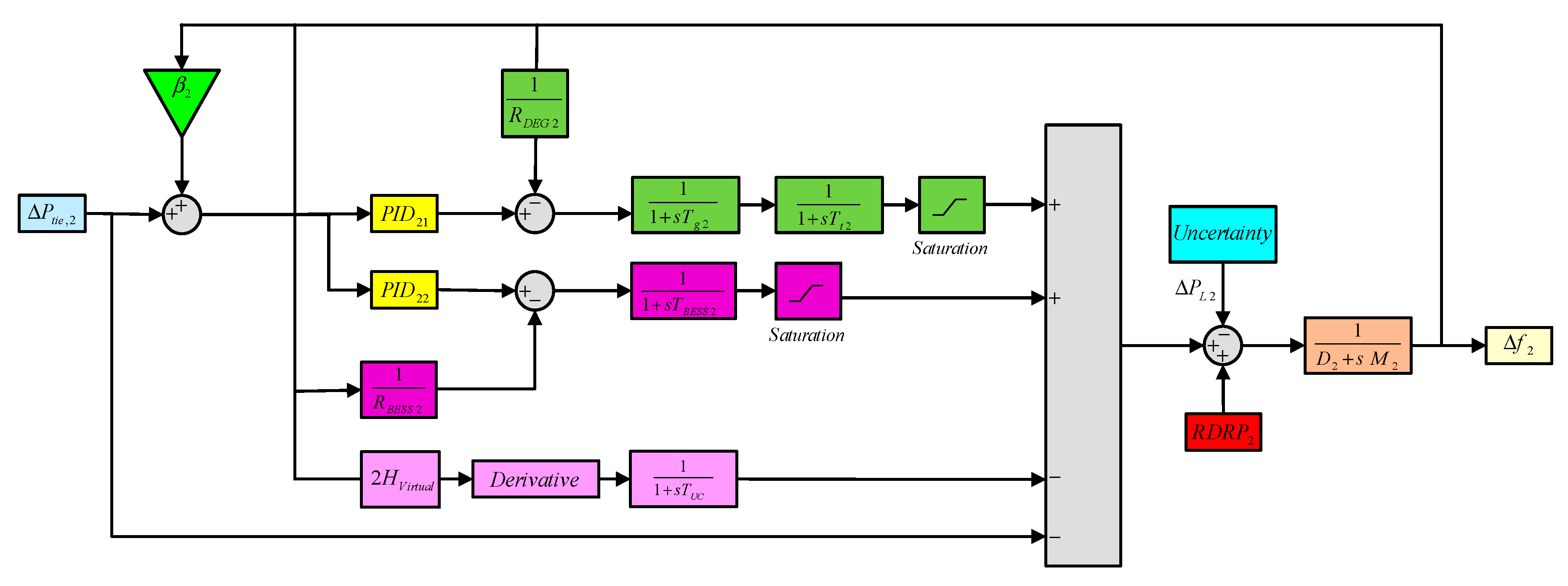
3. Modeling of Units

The modeling of the units, including DERs and ESSs, are presented below. The DERs consisted of a diesel engine generator, a fuel cell, a wind turbine generator, and a photovoltaic panel. The ESSs consisted of a flywheel energy storage system, a superconducting magnetic energy storage system, a battery energy storage system, and an ultracapacitor.

3.1. Modeling of the Diesel Engine Generator (DEG)

A DEG was used to compensate the microgrid required power by using a governor and a speed-drop system. The DEG conversion function is represented in Equation (1) [20]:

$$G_{DEG}(s)=\frac{-1}{R_{DEG}}(\frac{1}{1+s{T}_g}\times \frac{1}{1+s{T}_t}),$$

(1)

where T_g and T_t are the governor and turbine time constants, respectively. Furthermore, R_DEG is the speed regulation coefficient of the DEG. Generally, a power increment limitation block is considered for the DEG model.

3.2. Modeling of the Fuel Cell (FC)

The FC transforms the chemical energy stored in hydrogen into DC electrical energy. The FC begins to produce power by injecting hydrogen stored in its hydrogen tank. The model used for the FC was [40]:

$$G_{FC}(s)=\frac{1}{1+s{T}_{FC1}}\times \frac{1}{1+s{T}_{FC2}},$$

(2)

where T_FC1 and T_FC2 are the FC1 and FC2 feed time constants, respectively. The power generation increase rate limit was also applied for the FC model.

3.3. Modeling of the Wind Turbine (WT) Generator

In this study, the WT generator was not dispatchable. The WT generator was modeled as a specified random distribution. Furthermore, it was represented by the following transfer function [40]:

$$G_{WTG}(s)=\frac{1}{1+s{T}_{WTG}},$$

(3)

where T_WTG is the WT generator time constant.

3.4. Modeling of the Photovoltaic (PV) Panel

In this study, the PV panel was not dispatchable. The PV panel was modeled as a specified random distribution and it was modeled using the following transfer function [40]:

$$G_{PV}(s)=\frac{1}{1+s{T}_{PV}},$$

(4)

where T_PV is PV panel time constant.

3.5. Modeling of the Flywheel Energy Storage System (FESS)

The FESS plays an important role in a microgrid since it performs both the functions of releasing and storing energy at an appropriate time. Generally, a FESS is considered to provide mechanical energy. It is mostly identified using two various time constants: the electrical time constant and the mechanical time constant, which are identified by the electronic parts of the technology and the inertia of the system, respectively. The FESS generates active and reactive powers based on the angular speed of its rotational mass. Therefore, the speed control loop is added to the FESS model to provide an exact dynamic model of the FESS in the LFC scheme. As a mechanical rotational mass, the FESS has inertia. Due to the influence of the number of poles on the speed of this equipment, the number of poles should be applied to the mechanical part of this equipment [16].

The dynamic model of an FESS is represented in Figure 2, where T_F1, T_F2, and T_F3 are the time constants of the measurement device, command device, and converter, respectively. F₁ is a reference angular speed. F₂ is the speed regulator proportional constant. P_FESS is the number of poles of the FESS, and J_FESS is the inertia of the rotational masses of the FESS.

3.6. Modeling of the Superconducting Magnetic Energy Storage System (SMESS)

By injecting or absorbing power, an SMESS plays a significant role in increasing the frequency stability of the network. The exchange power of this unit is determined by the PI controller. This unit has a very small delay and it is modeled using a first-order conversion function that is described in Equation (5):

$$G_{SMESS}(s)=\frac{K_{SMESS}}{1+s{T}_{SMESS}},$$

(5)

where K_SMESS is the SMESS gain and T_SMESS is the SMESS time constant. Furthermore, the power generation increase and decrease rate limit are applied for the model [41].

3.7. Modeling of the Battery Energy Storage System (BESS)

A BESS is a basic voltage device that is used to prevent fluctuations in the power balance. The BESS conversion function is expressed in Equation (6):

$$G_{BESS}(s)=\frac{-1}{R_{BESS}}(\frac{1}{1+s{T}_{BESS}}).$$

(6)

T_BESS is the BESS time constant. Furthermore, R_BESS is the speed regulation coefficient of the BESS. The ramp-up and ramp-down rate of the output power of the BESS were also considered in this model [20].

3.8. Modeling of the Ultracapacitor (UC)

The UC plays a significant role in increasing the virtual inertia of the network via power absorption or injection. The exchange power of the UC with the network is directly dependent on the derivation of frequency fluctuations and it is represented by the following transfer function [19]:

$$G_{UC}(s)=\frac{1}{1+s{T}_{UC}},$$

(7)

where T_UC is the UC time constant.

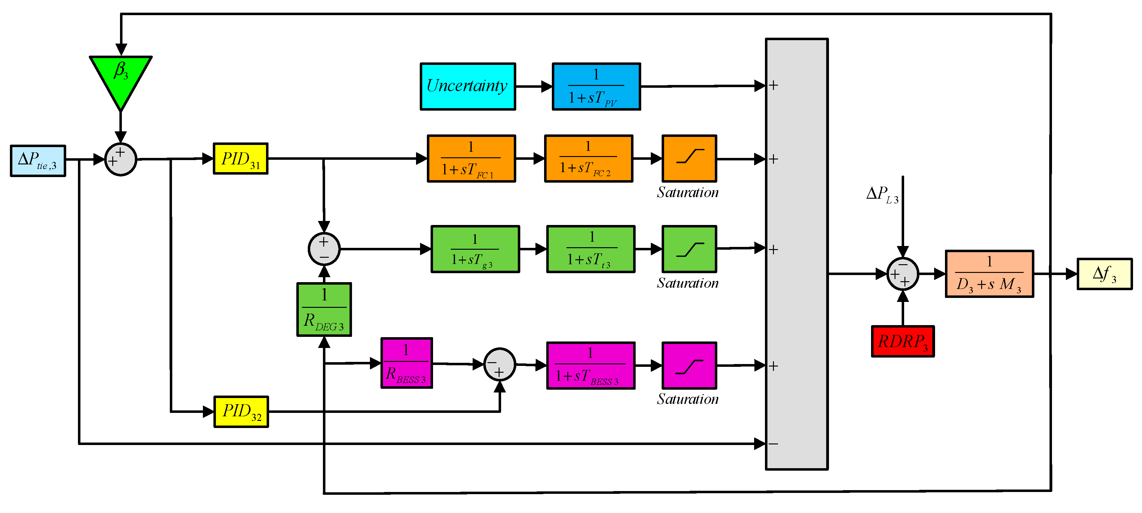
4. Modeling of the Microgrids

According to the presented dynamic models of each DER and ESS, and by considering the type of the resource of each microgrid, the dynamic models of the microgrids are shown in Figure 2, Figure 3 and Figure 4. In Figure 2, the block diagram of the dynamic model of microgrid 1 is illustrated, where ∆f₁ is the frequency deviation of microgrid 1, β₁ is frequency bias of microgrid 1, D₁ is the load-damping coefficient of microgrid 1, M₁ is the total inertia of microgrid 1, ∆P_L1 is the load change in microgrid 1, and ∆P_tie,1 is the total tie-line power change between microgrid 1 and the other microgrids. In Figure 3, the block diagram of the dynamic model of microgrid 2 is given, where ∆f₂ is the frequency deviation of microgrid 2, β₂ is the frequency bias of microgrid 2, D₂ is the load-damping coefficient of microgrid 2, M₂ is the total inertia of microgrid 2, ∆P_L2 is the load change in microgrid 2, and ∆P_tie,2 is the total tie-line power change between microgrid 2 and the other microgrids. In Figure 4, the block diagram of the dynamic model of microgrid 3 is demonstrated, where ∆f₃ is the frequency deviation of microgrid 3, β₃ is the frequency bias of microgrid 3, D₃ is the load-damping coefficient of microgrid 3, M₃ is the total inertia of microgrid 3, ∆P_L3 is the load change in microgrid 3, and ∆P_tie,3 is the total tie-line power change between microgrid 3 and the other microgrids.

The main parameters of microgrids 1–3 are given in

Table 1. Parameters of microgrid 1.

Parameter	Value	Parameter	Value	Parameter	Value	Parameter	Value
β1 (p.u./Hz) Tg1 (s) TSMESS (s) F1	10 0.05 0.3 1	D1 (p.u./Hz) Tt1 (s) TF1 (s) F2	1 0.5 0.1 0.5	M1 (p.u. s/Hz) RDEG1 (Hz/p.u.) TF2 (s) PFESS	3 0.05 0.1 4	TWTG (s) KSMESS TF3 (s) JFESS	0.04 0.98 0.01 2

,

Table 2. Parameters of microgrid 2.

Parameter	Value	Parameter	Value	Parameter	Value	Parameter	Value
β2 (p.u./HZ) Tt2 (s) HVirtual	10 0.4 0.139	D2 (p.u./Hz) RDEG2 (Hz/p.u.) TUC (s)	0.012 0.5682 0.2	M2 (p.u. s/Hz) TBESS2 (s)	0.298 0.1	Tg2 (s) RBESS2 (Hz/p.u.)	0.18 0.705

and

Table 3. Parameters of microgrid 3.

Parameter	Value	Parameter	Value	Parameter	Value	Parameter	Value
β3 (p.u./HZ) Tg3 (s) TFC2 (s)	10 0.08 0.04	D3 (p.u./Hz) Tt3 (s) TBESS3 (s)	0.015 0.4 0.08	M3 (p.u. s/Hz) RDEG3 (Hz/p.u.) RBESS3 (Hz/p.u.)	0.1667 3 3	TPV (s) TFC1 (s)	0.04 0.026

, respectively.

In the first microgrid, the WT generator did not participate in the frequency control. However, DEG, FESS, and SMESS participated in the frequency control. In the second microgrid, DEG and BESS were responsible for the power generation and the UC was used to inject or absorb power quickly to increase the virtual inertia of the microgrid. In addition, in the third microgrid, the PV generator did not participate in the frequency control. Nevertheless, the DEG, FC, and BESS participated in the frequency control. In each microgrid, two PID controllers were used for the LFC of the microgrids.

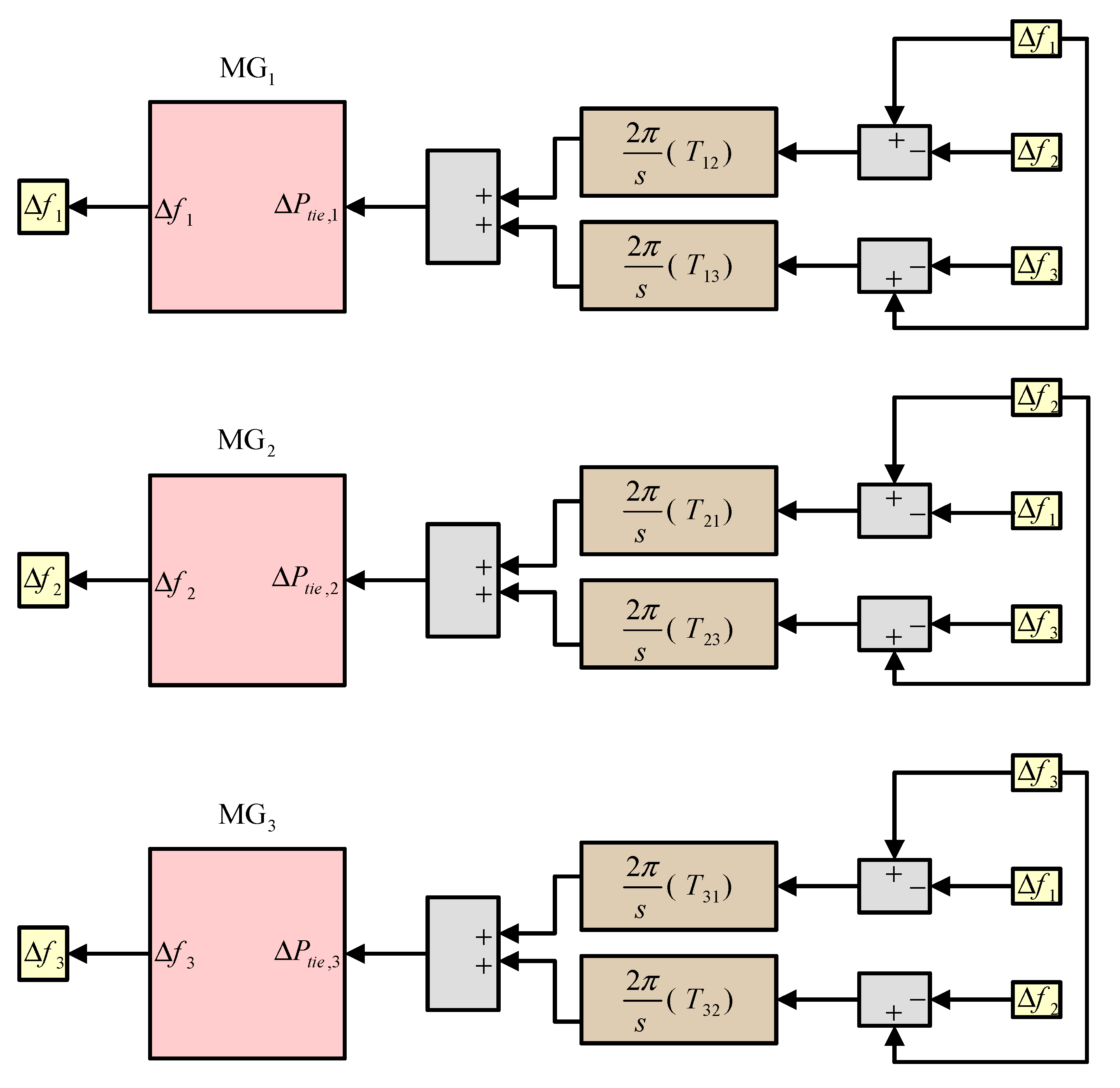
5. Modeling of the Multiple Microgrid Clusters

In this study, three microgrids were connected to each other with tie-lines. The exchanged tie-line power between two microgrids depends on the difference in frequency deviations of those microgrids and the tie-line synchronizing torque coefficient. Each of microgrids was connected to each other by two tie-lines and the total power of those two tie-lines was the exchange tie-line power of that microgrid. The dynamic model of multiple microgrid clusters is shown in Figure 5, where T₁₂, T₁₃, T₂₁, T₂₃, T₃₁, and T₃₂ are the tie-line synchronizing torque coefficients, which were set to T₁₂ = T₁₃ = T₂₁ = T₂₃ = T₃₁ = T₃₂ = 1.

6. Modeling of the Uncertainties

In power systems, there are many uncertainties and the definite parameters cannot indicate the exact status of these systems. Therefore, probabilistic analysis was considered as an attractive solution. In this study, RERs and load uncertainties were modeled with probability distribution functions.

6.1. Probabilistic Model of the Load

Weather conditions and time are two factors for the deterministic component of the load change. Due to the variable nature of the load, the random behavior of the load was suitable for modeling. This modeling could be calculated using measured data analysis. The load behavior was modeled using a normal distribution function. The normal distribution function is defined as following [42]:

$$f(P_L)={\frac{1}{\sqrt{2\pi }\times \sigma }}_{}{\exp }_{}(-\frac{{(P_L-\mu )}^2}{2\times {\sigma }^2}),$$

(8)

where P_L is the load power, μ is the mean, and σ is the standard deviation.

6.2. Probabilistic Model of the WT Power

The power produced by the WT generator depends on the wind speed. The wind speed changes regularly, which shows the significance of a probability model. The Weibull distribution function was used in modeling the wind speed. The Weibull distribution function is as follows [43]:

$$f(V)=\left\{\begin{array}{l}\frac{y}{x}\times {(\frac{V}{x})}^{y-1}\times \exp (-{(\frac{V}{x})}^y)\hspace{1em}V\ge 0\\ 0\hspace{1em}\hspace{1em}\hspace{1em}\hspace{1em}\hspace{1em}\hspace{1em}\hspace{1em}\hspace{1em}\mathrm{otherwise}\end{array}\right\},$$

(9)

where V is the wind speed, and y and x are the scale and shape parameters of the Weibull distribution function, respectively. After producing the wind speed samples, the real power generation by the WT generator can be acquired from the following equation:

$$P_{WT}(V)=\left\{\begin{array}{ll}0& 0\le V\le V_{ci}\hspace{0.17em}\mathit{\text{or}}\hspace{0.17em}V\ge V_{co}\\ P_{r,WT}\times \left(\frac{V^2-V_{ci}{}^2}{V_r-V_{co}{}^2}\right)& V_{ci}\le V\le V_r\\ P_{r,WT}& V_r\le V\le V_{co}\end{array}\right\},$$

(10)

where P_WT(V) is the power generated at wind speed V by the WT generator. P_r,WT is the rated power of the WT generator; V_ci, V_co, and V_r are the low cut speed, high cut speed, and rated speed of the WT generator, respectively.

6.3. Probabilistic Model of the PV Power

Solar radiation is one important parameter for power generation in the PV panel. This parameter is variable at any time of day. Thus, the location of the PV panel plays an essential role in generating electricity. The irradiance was modeled using the beta distribution function. The PV panel was tested under the standard test condition (STC). After radiation sampling, the final power output of the PV panel was calculated as follows [44]:

$$P_{PV}(R)=\left\{\begin{array}{ll}{P}_{r,PV}\times {\left(\frac{R^2}{R_{STC}\times R_C}\right)}_{}^{}& 0\le R\le R_C\\ P_{r,PV}\times {\left(\frac{R}{R_{STC}}\right)}_{}^{}& R_C\le R\le R_{STC}\\ P_{r,PV}& R_{STC}\le R\end{array}\right\},$$

(11)

where P_PV(R) is the power generated by the PV panel; P_r,PV is the rated power of the PV panel; and R, R_C, and R_STC are the solar radiation, certain radiation point, and the solar radiation under the STC, respectively.

6.4. Scenario Generation and Reduction

The uncertainty of the input parameters, including the generation of RERs and the load demands, was considered by applying the scenario generation. For the uncertainty parameters, a Monte Carlo simulation was used to generate scenarios. Based on Hemmati [45], probability distribution sets were used to model the uncertainties. To reduce the complexity of the problems, a scenario reduction method was utilized. The scenario reduction is a method used for reducing the implementation time of the simulation [46].

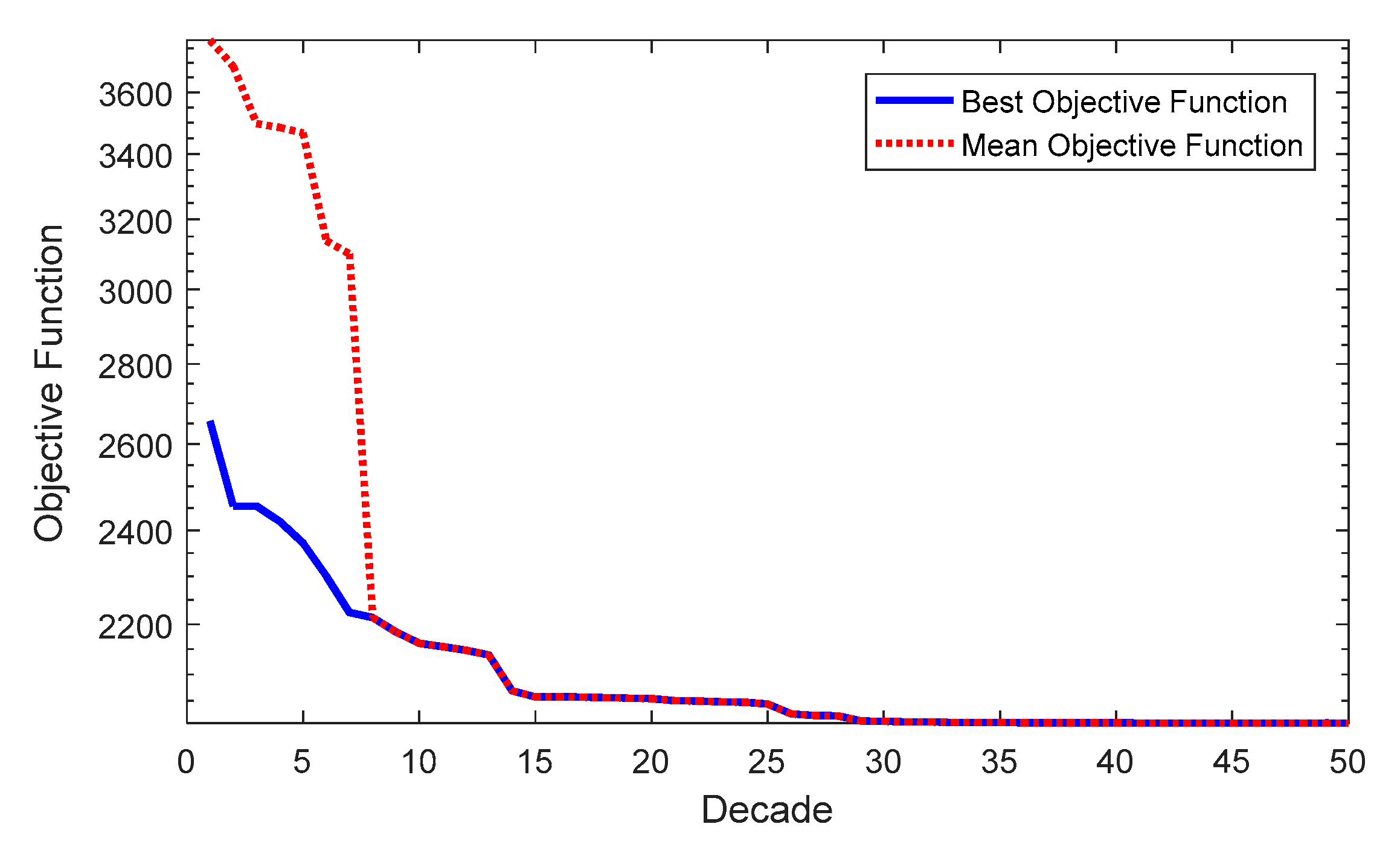
6.5. Imperialist Competitive Algorithm

Since there are many variables and control signals, we needed to use optimization algorithms to adjust the control parameters. For these algorithms, the specific objective functions must be defined. The objective functions should be optimized according to the constraints to determine the optimal value of the control parameters. In this study, the ICA was used as described below.

The ICA is an evolutionary optimization method. Similar to other evolutionary methods, the ICA produces some random initial population, which is named “country.” It is separated into two types, imperialists and colonies, which together form empires. The stages of the suggested algorithm are described as follows: the generation of initial empires, the assimilation, the revolution, the exchange between the best colony and imperialist, the imperialistic competition, and the elimination of a powerless empire [47].

7. Modeling of Regional Demand Response Programs

Based on Babahajiani et al. [39], an algorithm was utilized for applying the RDRPs in frequency control. The proposed solution involved monitoring the deviations of the tie-line flows, computed the magnitude of the disturbances, and synchronously specified the microgrid where disturbances occurred to apply the demand response programs exactly to the involved microgrid. The proposed algorithm is given as follows:

$$RDR{P}_i=\frac{-M_i\frac{d^2}{d{t}^2}\mathsf{\Delta }{P}_{tie,i}(t)}{2\pi {\displaystyle \sum _{j=1_{}^{}{,}_{}^{}j\ne i}^N{T}_{ij}}}\times {\gamma }_i.$$

(12)

At first, the second derivative of the tie-line flows of all microgrids was computed. Some of the demand response programs were voluntary and contract-based. Therefore, when applying the impact of this limitation, the participation factor 0 < γ < 1 in Equation (12) was considered. The participation factor determines how much load could participate in the demand response programs at the time of disturbance. γ = 0 means that no loads participate in frequency control and γ = 1 means that all active loads participate in frequency control. The Federal Energy Regulatory Commission (FERC) in the United States has announced that the residential controlled loads, such as refrigerators, water heaters, air conditioners, and heat pumps, make up about 20% of the total electricity consumption in the United States [48]. Furthermore, in Bao and Li [49], it has been declared that electric heaters use about 11% of the total electricity consumption. In this study, for evaluating the proposed algorithm, it was supposed that in each microgrid, 30% of loads were controllable by the demand response programs. The proposed solution in this work was considered as a direct load control (DLC) that was usually voluntary and contract-based. Figure 6 displays how the RDRPs contribute to the frequency control, where ΔP_tie,i is the total tie-line power change between microgrid i and the other microgrids, γ_i is the participation factor of demand response programs of microgrid i, τ_i is the demand response programs time delay of microgrid i, and RDRP_i is the calculated load for the demand response programs of microgrid i.

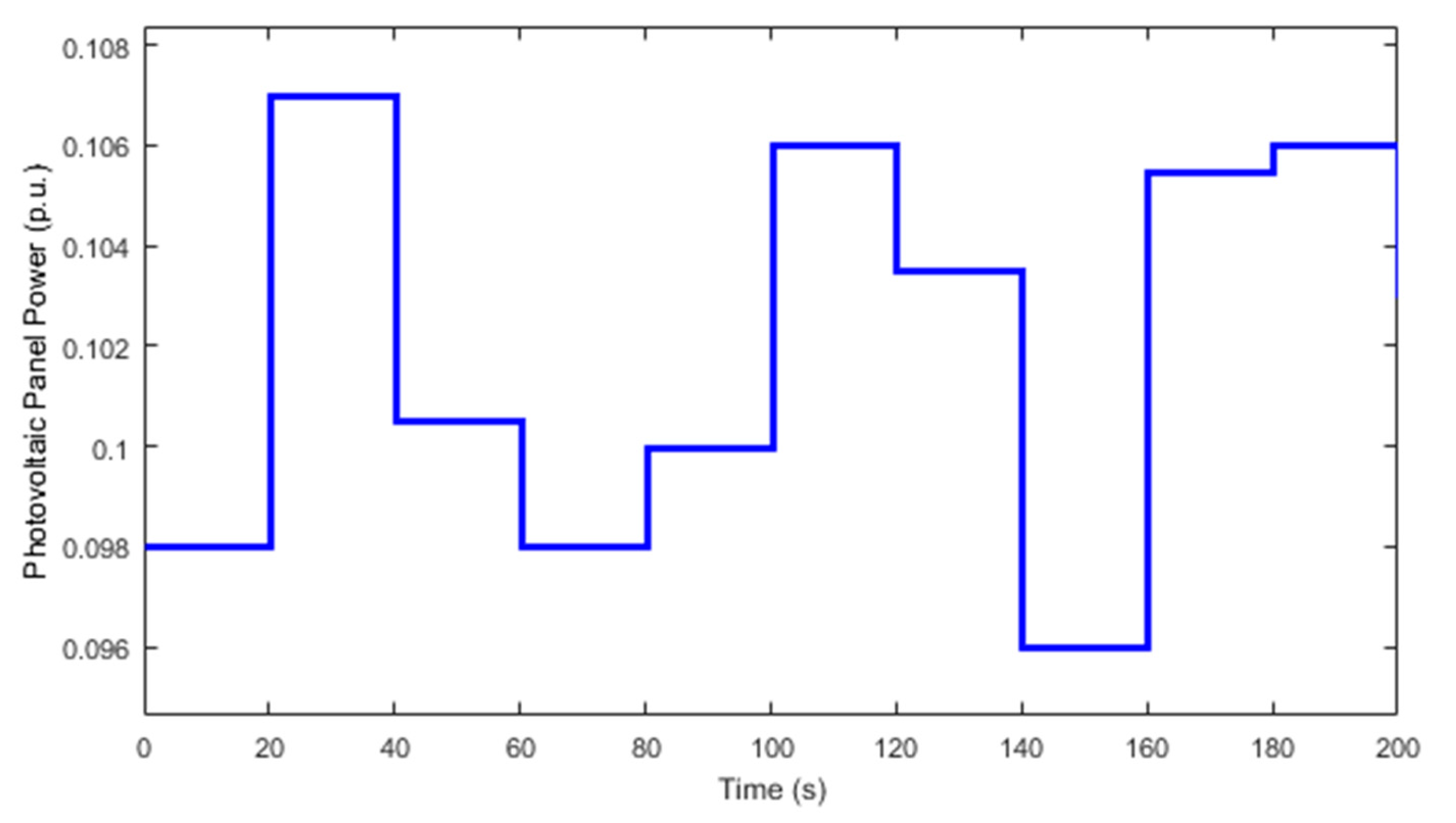
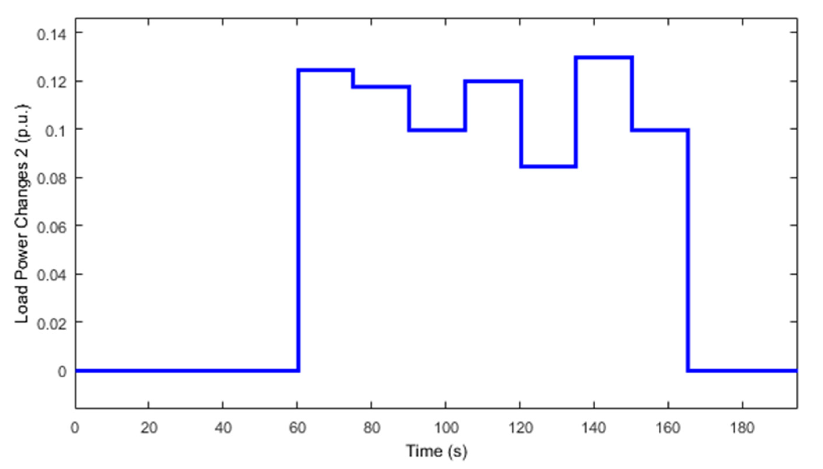
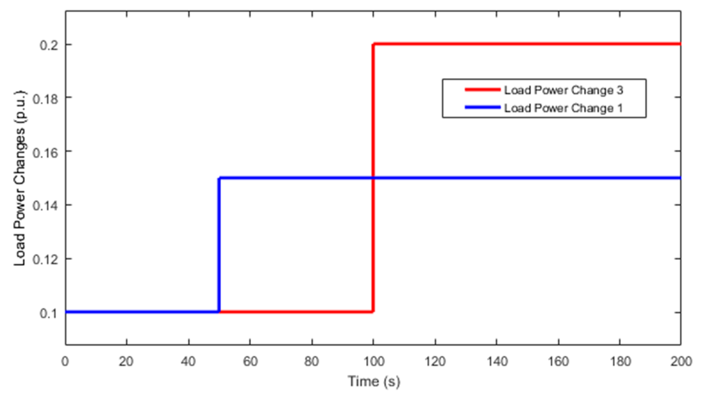
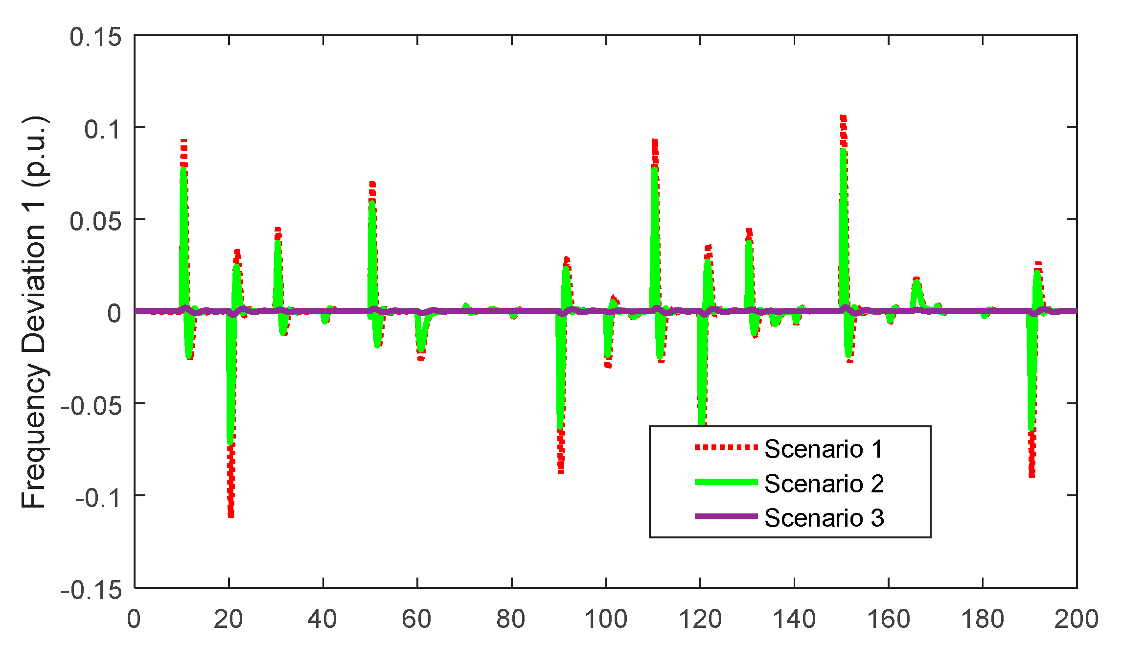
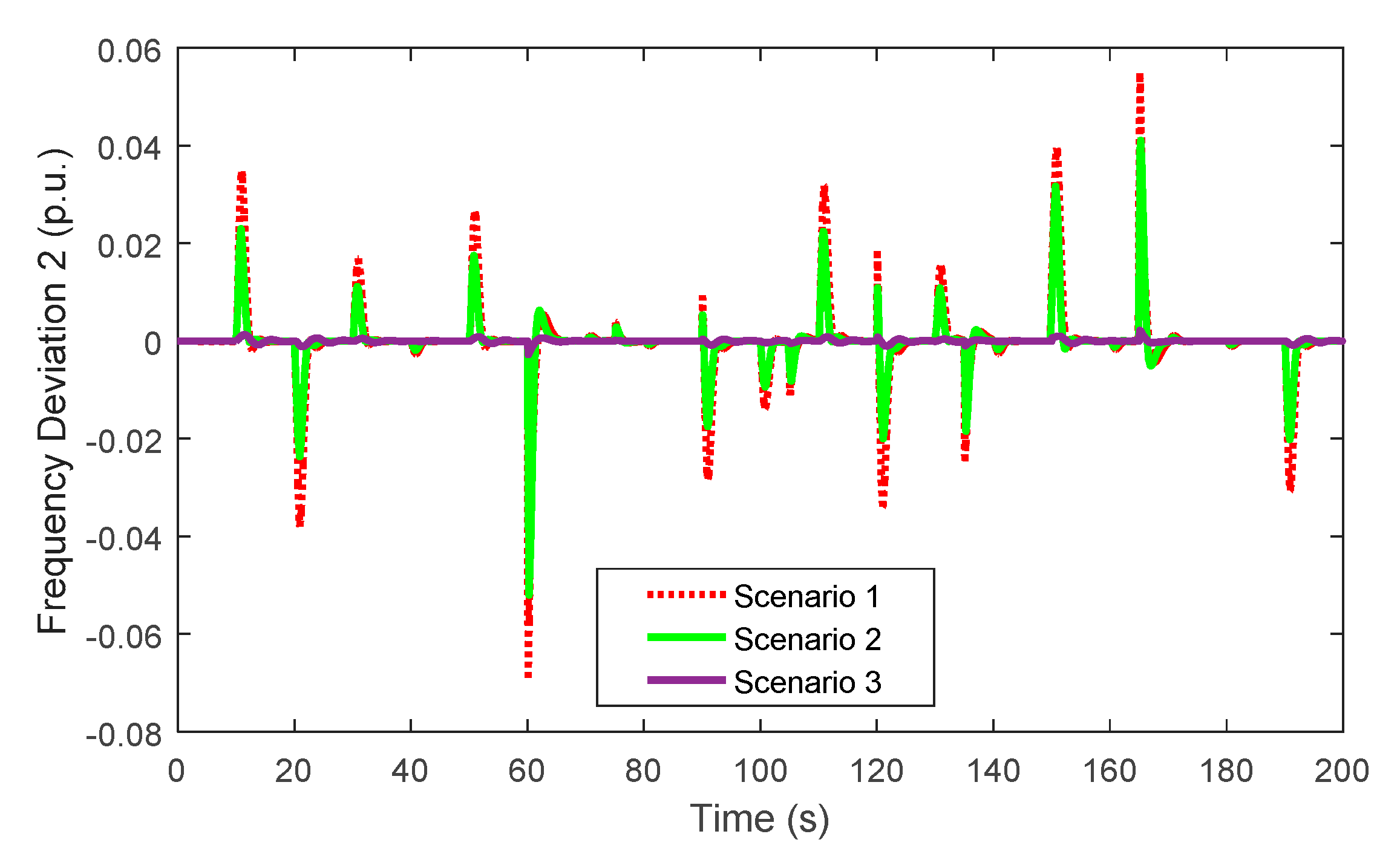
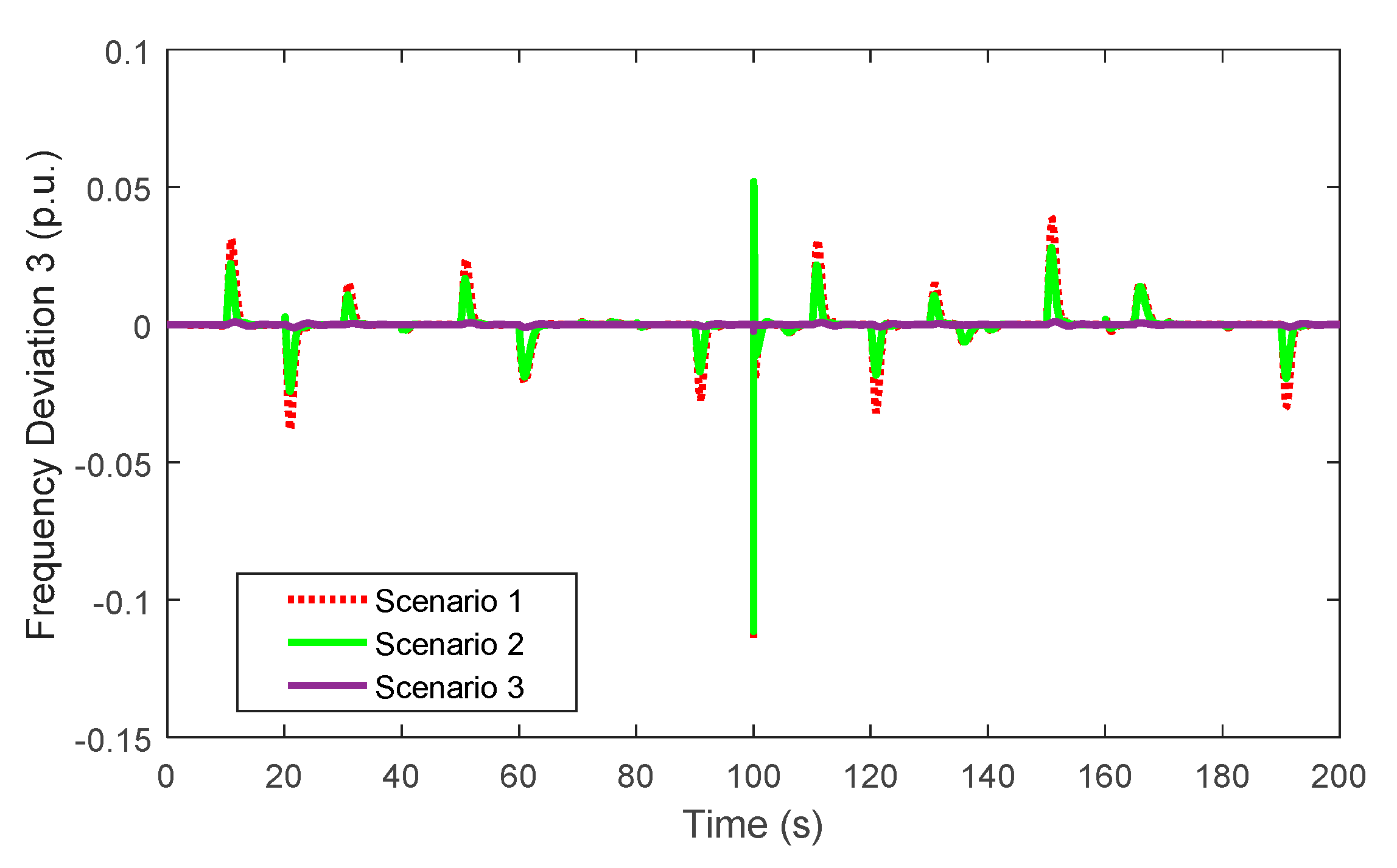
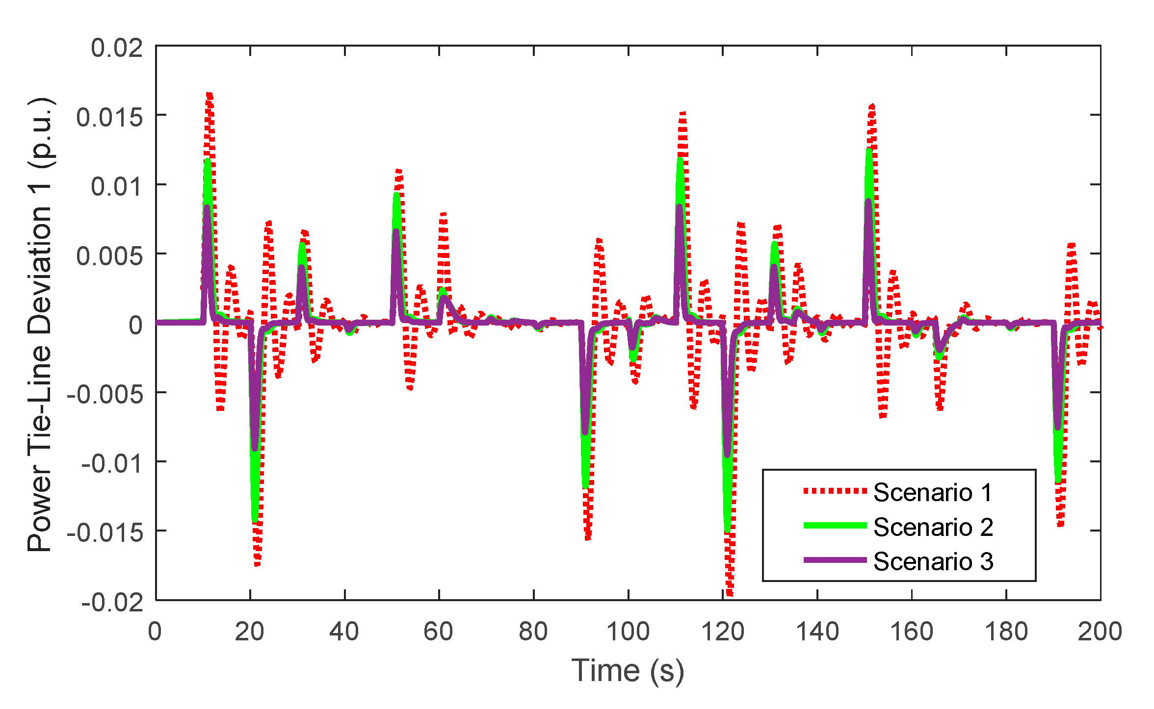
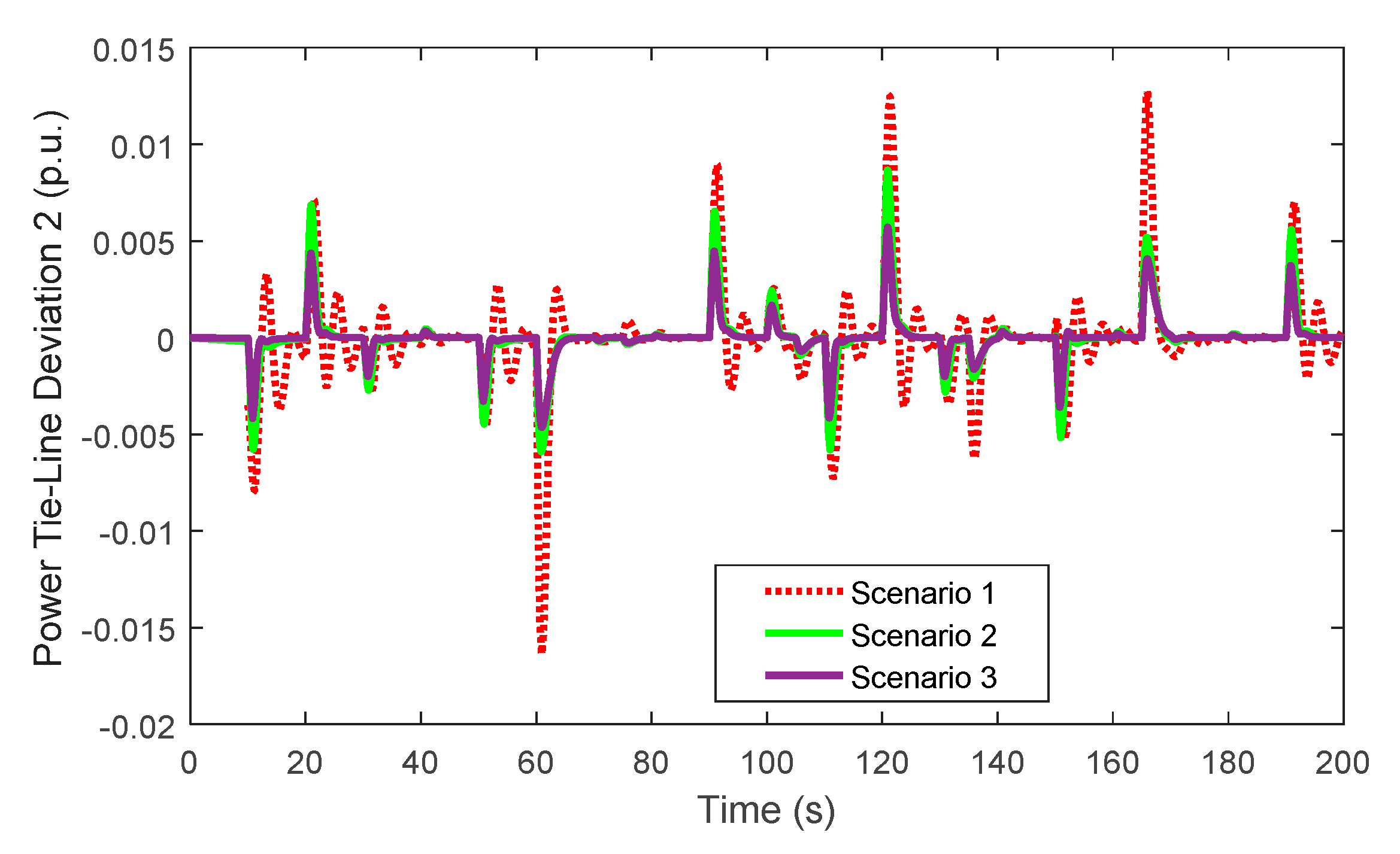
8. Simulation Results and Discussions

The frequency control system of multiple microgrid clusters was implemented in Matlab R2016b/Simulink software. To investigate the proposed methods, three scenarios were examined:

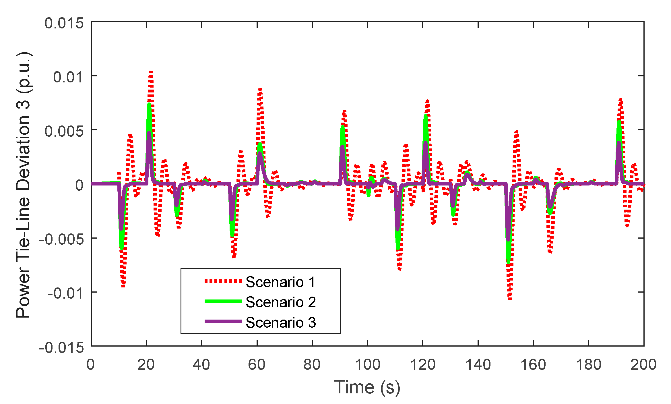
• Scenario 1: In the first scenario, the performance of the multiple microgrid clusters was studied with non-optimal parameter values.
• Scenario 2: In the second scenario, the performance of the multiple microgrid clusters was examined with the optimal control parameters.
• Scenario 3: In the third scenario, the performance of the multiple microgrid clusters was investigated by applying RDRPs.

These scenarios show the effectiveness of the selected solutions at overcoming frequency deviations and power tie-line deviations. In all the scenarios, the RERs and loads uncertainties were considered in the same profile. In the first microgrid, the production of the WT generator had uncertainty and it was modeled using the Weibull distribution function. In the second microgrid, the power load had uncertainty and it was modeled using a normal distribution function. In the third microgrid, the production of the PV panel had uncertainty and it was modeled using the beta distribution function. By applying uncertainties, the output powers of the WT generator and the PV panel were generated and are shown in Figure 7 and Figure 8, respectively. In addition, the power load uncertainty is shown in Figure 9.

Furthermore, the magnitude of the load demand in the first microgrid at t = 50 (s) was equal to 0.05 per unit and the magnitude of the load demand in the third microgrid at t = 100 (s) was equal to 0.1 per unit. Figure 10 shows the load power changes of microgrids 1 and 3.

By applying the uncertainties, the frequency deviations of the microgrids, non-optimal and optimal parameters, and RDRPs were simulated and the results of these simulations are shown in Figure 11, Figure 12 and Figure 13.

By applying uncertainties, the exchange tie-line power deviations between the microgrids, non-optimal and optimal parameters, and RDRPs were simulated and are shown in Figure 14, Figure 15 and Figure 16.

In the first scenario, the PID controllers were used for the LFC of the microgrids and the non-optimal parameters were acquired using a trial and error method. The non-optimal values are given in

Table 4. Non-optimal control parameter values.

Parameter	Value	Parameter	Value	Parameter	Value
Kp11 Kp12 Ki11 Ki12 Kd11 Kd12	−0.0083 −1.972 −4.9991 −4.996 −4.1601 −2.6442	Kp21 Kp22 Ki21 Ki22 Kd21 Kd22	−2.0719 −0.1249 −3.605 −0.15 −1.7581 −0.5424	Kp31 Kp32 Ki31 Ki32 Kd31 Kd32	−4.09 −4.09 −2.1081 −2.1081 −1 −1

, where K_p is a proportional gain parameter, K_i is an integral gain parameter, and K_d is a differential gain parameter, and the subscript numbers refer to the relevant microgrids.

In the second scenario, the system parameters were acquired using the ICA. The ICA was used to optimize one objective. The goal was to reduce the sum of the frequency deviations of the microgrids and the tie-line power deviations between microgrids. The objective function is given as:

$$Objective Function={\displaystyle \underset{0}{\overset{t}{\int }}[(\mathsf{\Delta }{f}_1(\tau )+\mathsf{\Delta }{f}_2(\tau )+\mathsf{\Delta }{f}_3(\tau ))}+(\mathsf{\Delta }{P}_{tie,1}(\tau )+\mathsf{\Delta }{P}_{tie,2}(\tau )+\mathsf{\Delta }{P}_{tie,3}(\tau )){]}^{}{\tau }^{}d\tau .$$

(13)

The performance of the convergence curve is shown in Figure 17.

The optimal values are given in

Table 5. Optimal control parameter values.

Parameter	Value	Parameter	Value	Parameter	Value
Kp11 Kp12 Ki11 Ki12 Kd11 Kd12	−0.042 −3.9327 −7.9876 −7.8101 −4.815 −3.1939	Kp21 Kp22 Ki21 Ki22 Kd21 Kd22	−4.8144 −3.2097 −4.8601 −1.8405 −2.9884 −0.8321	Kp31 Kp32 Ki31 Ki32 Kd31 Kd32	−5.6655 −5.6655 −3.4699 −3.4699 −2.951 −2.951

.

The ICA parameters are listed in

Table 6. ICA parameters.

Parameter	Value
Number of iterations or decades Number of initial countries Number of imperialist countries Number of colonies	50 17 5 12

.

The upper and lower limits of the variables are listed in

Table 7. The ranges of the parameter limitations.

Parameter	Limitation	Parameter	Limitation	Parameter	Limitation
Kp11 Kp12 Ki11 Ki12 Kd11 Kd12	−0.1 to −0.05 −5 to −1 −10 to −2 −10 to −1 −10 to −2 −5 to −1	Kp21 Kp22 Ki21 Ki22 Kd21 Kd22	−5 to −1 −5 to −0.5 −5 to −1 −2 to −0.05 −5 to −0.5 −2 to −0.1	Kp31 Kp32 Ki31 Ki32 Kd31 Kd32	−10 to −1 −10 to −1 −5 to −1 −5 to −1 −5 to −0.1 −5 to −0.1

.

According to the simulation results, the frequency deviations of the microgrid and the tie-line power deviations between the microgrids were reduced with the application of the optimal parameters. Tuning the non-optimal parameters with the ICA algorithm decreased the overshoots and undershoots of the frequency deviations and the tie-line power deviations.

In the third scenario, the RDRPs were applied to each microgrid. It was supposed that, in each microgrid, 30% of the loads were available for the demand response programs. Therefore, the participation factor (γ) in each microgrid was equal to 0.3. The demand response time delay in each microgrid was considered to be 0.5 s.

The frequency behavior of the microgrids shown in Figure 11, Figure 12 and Figure 13 indicates that applying the RDRPs improved the damping of frequency fluctuations.

9. Conclusions

Frequency control is one of the most important challenges facing multiple microgrid clusters. To study frequency control, an appropriate dynamic model is necessary. A dynamic model of multiple microgrid clusters with different types of DERs and ESSs, including a DEG, an FC, a WT generator, a PV panel, an FESS, an SMESS, a BESS, and a UC, and based on tie-lines, was introduced in this paper. It was found that tuning the control parameters with intelligent algorithms, such as the ICA, was the best method. The result of this research showed that tuning the control parameters with the ICA could decrease the overshoots and undershoots of frequency deviations. Improving the frequency stability is another challenge facing multiple microgrid clusters. In this study, applying the RDRPs improved the frequency stability of the microgrids. To study the multiple microgrid clusters, simulations were performed in Matlab/Simulink software. Investigation results have demonstrated the effectiveness of the best proposed solutions at overcoming frequency fluctuations. For future work, designing adaptive controllers is suggested.

References

1. Dong, J.; Xue, G.; Dong, M.; Xu, X. Energy saving power generation dispatching in China: Regulations, pilot projects and policy recommendations-a review. Renew. Sustain. Energy Rev. 2015, 44, 1285–1300. [Google Scholar] [CrossRef]
2. Bull, S.R. Renewable energy today and tomorrow. Proc. IEEE 2001, 89, 1216–1226. [Google Scholar] [CrossRef]
3. Mahzarnia, M.; Sheikholeslami, A.; Adabi, J. A voltage stabilizer for a microgrid system with two types of distributed generation resources. IIUM Eng. J. 2013, 14, 191–205. [Google Scholar] [CrossRef]
4. Su, C.-L. Effects of distribution system operations on voltage profiles in distribution grids connected wind power generation. In Proceedings of the 2006 International Conference on Power System Technology, Chongqing, China, 22–26 October 2006; pp. 1–7. [Google Scholar]
5. Ausavanop, O.; Chaitusaney, S. Coordination of dispatchable distributed generation and voltage control devices for improving voltage profile by Tabu search. In Proceedings of the 8th Electrical Engineering/Electronics, Computer, Telecommunications and Information Technology (ECTI), Khon Kaen, Thailand, 17–19 May 2011; pp. 869–872. [Google Scholar]
6. Sekhar, A.S.R.; Krishna, K.V. Improvement of voltage profile of the hybrid power system connected to the grid. Int. J. Eng. Res. Appl. 2012, 2, 087–093. [Google Scholar]
7. Chang, X.; Li, Y.; Zhang, W.; Wang, N.; Xue, W. Active disturbance rejection control for a flywheel energy storage system. IEEE Trans. Ind. Electron. 2015, 62, 991–1001. [Google Scholar] [CrossRef]
8. Vazquez, S.; Lukic, S.M.; Galvan, E.; Franquelo, L.G.; Carrasco, J.M. Energy storage systems for transport and grid applications. IEEE Trans. Ind. Electron. 2010, 57, 3881–3895. [Google Scholar] [CrossRef] [Green Version]
9. Hatziargyriou, N. Microgrids: Architectures and Control; John Wiley and Sons: Hoboken, NJ, USA, 2014. [Google Scholar]
10. Valenciaga, F.; Puleston, P.F. Supervisor control for a stand-alone hybrid generation system using wind and photovoltaic energy. IEEE Trans. Energy Convers. 2005, 20, 398–405. [Google Scholar] [CrossRef]
11. Lee, D.-J.; Wang, L. Small signal stability analysis of an autonomous hybrid renewable energy power generation/energy storage system part I: Time-domain simulations. IEEE Trans. Energy Convers. 2008, 23, 311–320. [Google Scholar] [CrossRef]
12. Senjyo, T.; Nakaji, T.; Uezato, K.; Funabashi, T. A hybrid power system using alternative energy facilities in isolated island. IEEE Trans. Energy Convers. 2005, 20, 406–414. [Google Scholar] [CrossRef]
13. Majumder, R.; Chaudhuri, B.; Ghosh, A.; Majumder, R.; Ledwich, G.; Zare, F. Improvement of stability and load sharing in an autonomous microgrid using supplementary droop control loop. IEEE Trans. Power Syst. 2010, 25, 796–808. [Google Scholar] [CrossRef] [Green Version]
14. Diaz, G.; Gonzalez-Moran, C.; Gomez-Aleixandre, J.; Diez, A. Scheduling of droop coefficients for frequency and voltage regulation in isolated microgrids. IEEE Trans. Power Syst. 2010, 25, 489–496. [Google Scholar] [CrossRef]
15. Ayaz, M.S.; Azizipanah-Abarghooee, R.; Terzija, V. European LV microgrid benchmark network: Development and frequency response analysis. In Proceedings of the 2018 IEEE International Energy (ENERGYCON), Limassol, Cyprus, 3–7 June 2018. [Google Scholar]
16. Abazari, A.; Monsef, H.; Wu, B. Coordination strategies of distributed energy resources including FESS, DEG, FC and WTG in load frequency control (LFC) scheme of hybrid isolated microgrid. Int. J. Electr. Power Energy Syst. 2019, 109, 535–547. [Google Scholar] [CrossRef]
17. Mishra, S.; Mallesham, G.; Jha, A.N. Design of controller and communication for frequency regulation of a smart microgrid. IET Renew. Power Gener. 2012, 6, 248–258. [Google Scholar] [CrossRef]
18. Abdel-Hamed, A.M.; Ellissy, A.E.; El-Wakeel, A.S.; Abdelaziz, A.Y. Optimized control scheme for frequency/power regulation of microgrid for fault tolerant operation. Electr. Power Compon. Syst. 2016, 44, 1429–1440. [Google Scholar] [CrossRef]
19. Alizadeh, G.A.; Rahimi, T.; Nozadian, M.H.B.; Padmanaban, S.; Leonowic, Z. Improving microgrid frequency regulation based on the virtual inertia concept while considering communication system delay. Energies 2019, 12, 2016. [Google Scholar] [CrossRef] [Green Version]
20. Fini, M.H.; Golshan, M.E.H. Determining optimal virtual inertia and frequency control parameters to preserve the frequency stability in islanded microgrids with high penetration of renewables. Electr. Power Syst. Res. 2018, 154, 13–22. [Google Scholar] [CrossRef]
21. Shahidehpour, M.; Li, Z.; Bahramirad, S.; Li, Z.; Tian, W. Networked microgrids: Exploring the possibilities of the IIT-Bronzeville grid. IEEE Power Energy Mag. 2017, 15, 63–71. [Google Scholar] [CrossRef]
22. Toro, V.; Mojica-Nava, E. Droop free control for networked microgrids. In Proceedings of the 2016 IEEE Conference on Control Applications (CCA), Buenos Aires, Argentina, 19–22 September 2016. [Google Scholar]
23. Panda, S.; Yegireddy, N.K. Automatic generation control of multi area power system using multi objective non dominated sorting genetic algorithm II. Int. J. Electr. Power Energy Syst. 2013, 53, 54–63. [Google Scholar] [CrossRef]
24. Arya, Y. Automatic generation control of two area electrical power systems via optimal fuzzy classical controller. J. Frankl. Inst. 2018, 355, 2662–2688. [Google Scholar] [CrossRef]
25. Medina, J.; Muller, N.; Roytelman, I. Demand response and distribution grid operations: Opportunities and challenges. IEEE Trans. Smart Grid 2010, 1, 193–198. [Google Scholar] [CrossRef]
26. Aunedi, M.; Kountouriotis, P.A.; Calderon, J.E.O.; Angeli, D.; Strbac, G. Economic and environmental benefits of dynamic demand in providing frequency regulation. IEEE Trans. Smart Grid 2013, 4, 2036–2048. [Google Scholar] [CrossRef]
27. Losi, A.; Mancarella, P.; Vicino, A. Integration of Demand Response into the Electricity Chain: Challenges, Opportunities, and Smart Grid Solutions; John Wiley & Sons: Hoboken, NJ, USA, 2015. [Google Scholar]
28. Moghadam, M.R.V.; Ma, R.T.B.; Zhang, R. Distributed frequency control in smart grids via randomized demand response. IEEE Trans. Smart Grid 2014, 5, 2798–2809. [Google Scholar] [CrossRef]
29. Rezaei, N.; Kalantar, M. Smart microgrid hierarchical frequency control ancillary service provision based on virtual inertia concept: An integrated demand response and droop controlled distributed generation framework. Energy Convers. Manag. 2015, 92, 287–301. [Google Scholar] [CrossRef]
30. Rezaei, N.; Kalantar, M. Stochastic frequency security constrained energy and reserve management of an inverter interfaced islanded microgrid considering demand response programs. Int. J. Electr. Power Energy Syst. 2015, 69, 273–286. [Google Scholar] [CrossRef]
31. Huang, H.; Li, F. Sensitivity analysis of load damping characteristic in power system frequency regulation. IEEE Trans. Power Syst. 2013, 28, 1324–1335. [Google Scholar] [CrossRef]
32. Malik, A.; Ravishankar, J. A hybrid control approach for regulating frequency through demand response. Appl. Energy 2018, 210, 1347–1362. [Google Scholar] [CrossRef]
33. Soares, J.; Ghazvini, M.A.F.; Borges, N.; Vale, Z. A stochastic model for energy resources management considering demand response in smart grids. Electr. Power Syst. Res. 2017, 143, 599–610. [Google Scholar] [CrossRef] [Green Version]
34. Chang-Chien, L.R.; An, L.N.; Lin, T.W.; Lee, W.J. Incorporating demand response with spinning reserve to realize an adaptive frequency restoration plan for system contingencies. IEEE Trans. Smart Grid 2012, 3, 1145–1153. [Google Scholar] [CrossRef]
35. Zhao, C.; Topcu, U.; Low, S.H. Optimal load control via frequency measurement and neighborhood area communication. IEEE Trans. Power Syst. 2013, 28, 3576–3587. [Google Scholar] [CrossRef] [Green Version]
36. Ford, J.J.; Bevrani, H.; Ledwich, G. Adaptive load shedding and regional protection. Int. J. Electr. Power Energy Syst. 2009, 31, 611–618. [Google Scholar] [CrossRef]
37. Bayat, M.; Sheshyekani, K.; Hamzeh, M.; Rezazadeh, A. Coordination of distributed energy resources and demand response for voltage and frequency support of MV microgrids. IEEE Trans. Power Syst. 2016, 31, 1506–1516. [Google Scholar] [CrossRef]
38. Gao, W.; Ning, J. Wavelet based disturbance analysis for power system wide area monitoring. IEEE Trans. Smart Grid 2011, 2, 121–130. [Google Scholar] [CrossRef]
39. Babahajiani, P.; Shafiee, Q.; Bevrani, H. Intelligent demand response contribution in frequency control of multi area power systems. IEEE Trans. Smart Grid 2016, 9, 1282–1291. [Google Scholar] [CrossRef]
40. Bevrani, H.; Habibi, F.; Babahajyani, P.; Watanabe, M.; Mitani, Y. Intelligent frequency control in an AC microgrid: Online PSO based fuzzy tuning approach. IEEE Trans. Smart Grid 2012, 3, 1935–1944. [Google Scholar] [CrossRef]
41. Ortega, A.; Milano, F. Generalized model of VSC based energy storage systems for transient stability analysis. IEEE Trans. Power Syst. 2016, 31, 3369–3380. [Google Scholar] [CrossRef] [Green Version]
42. Nikmehr, N.; Ravadanegh, S.N. Optimal power dispatch of multi microgrids at future smart distribution grids. IEEE Trans. Smart Grid 2015, 6, 1648–1657. [Google Scholar] [CrossRef]
43. Nikmehr, N.; Ravadanegh, S.N. Heuristic probabilistic power flow algorithm for microgrids operation and planning. IET Gener. Transm. Distrib. 2015, 9, 985–995. [Google Scholar] [CrossRef]
44. Nikmehr, N.; Ravadanegh, S.N. Optimal operation of distributed generations in microgrids under uncertainties in load and renewable power generation using heuristic algorithm. IET Renew. Power Gener. 2015, 9, 982–990. [Google Scholar] [CrossRef]
45. Hemmati, R. Technical and economic analysis of home energy management system incorporating small scale wind turbine and battery energy storage system. J. Clean. Prod. 2017, 159, 106–118. [Google Scholar] [CrossRef]
46. Salehi, J.; Abdolahi, A. Optimal scheduling of active distribution networks with penetration of PHEV considering congestion and air pollution using DR program. Sustain. Cities Soc. 2019, 51, 1–15. [Google Scholar] [CrossRef]
47. Nikmehr, N.; Ravadanegh, S.N. Stochastic risk and reliability assessments of energy management system in grid of microgrids under uncertainty. J. Power Technol. 2017, 97, 179–189. [Google Scholar]
48. U.S. Energy Information Administration: Annual Energy Review. Available online: http://www.eia.gov/totalenergy/data/annual/#consumption (accessed on 16 April 2020).
49. Bao, Y.-Q.; Li, Y. FPGA based design of grid friendly appliance controller. IEEE Trans. Smart Grid 2014, 5, 924–931. [Google Scholar] [CrossRef]
Figure 1. Studied multiple microgrid clusters.
Energies 13 04050 g001
Figure 2. Dynamic model of microgrid 1. PID: Proportional integral derivative, RDRP: Regional demand response program.
Energies 13 04050 g002
Figure 3. Dynamic model of microgrid 2.
Energies 13 04050 g003
Figure 4. Dynamic model of microgrid 3.
Energies 13 04050 g004
Figure 5. Dynamic model of the multiple microgrid clusters.
Energies 13 04050 g005
Figure 6. Modeling of the RDRPs.
Energies 13 04050 g006
Figure 7. Wind turbine generator output power
Energies 13 04050 g007
Figure 8. Photovoltaic panel output power.
Energies 13 04050 g008
Figure 9. Load power.
Energies 13 04050 g009
Figure 10. Load power changes of microgrids 1 and 3.
Energies 13 04050 g010
Figure 11. Comparison of the frequency deviations of microgrid 1 in the three scenarios.
Energies 13 04050 g011
Figure 12. Comparison of the frequency deviations of microgrid 2 in the three scenarios.
Energies 13 04050 g012
Figure 13. Comparison of the frequency deviations of microgrid 3 in the three scenarios.
Energies 13 04050 g013
Figure 14. Comparison of the exchange tie-line power deviations between microgrids 1 and 2 in the three scenarios.
Energies 13 04050 g014
Figure 15. Comparison of the exchange tie-line power deviations between microgrids 2 and 3 in the three scenarios.
Energies 13 04050 g015
Figure 16. Comparison of the exchange tie-line power deviations between microgrids 3 and 1 in the three scenarios.
Energies 13 04050 g016
Figure 17. Performance of the convergence curve using the imperialist competitive algorithm (ICA).
Energies 13 04050 g017