1. Introduction
Advances in intelligent transport systems along with the automation of the vehicles have enabled the development of vehicle platooning strategies in which a group of vehicles follow each other in a close and coordinated way [
1], primarily to increase road capacity [
2] and reduce overall energy consumption. With improvements in sensor and communication technologies, vehicles can be electronically coupled and controlled to drive together at closer distances in a platoon, thereby reducing the energy consumption due to the aerodynamic advantage of driving in close proximity [
3]. Aerodynamic drag is one of the major contributors to the energy consumption of a vehicle and increases quadratically with the increase in vehicle speed. The aerodynamic drag of a vehicle comprises of skin friction drag and pressure drag [
4]. The pressure drag, which is the major contributor to the overall drag, arises due to the pressure difference between the high pressure region at the front of the vehicle and the low pressure region at the rear of the vehicle. When a vehicle is driven in a platoon, the pressure difference on the vehicle is reduced. Platooning therefore decreases the aerodynamic drag and consequently improves the energy efficiency of the vehicle.
The aerodynamics of vehicle platooning have been extensively studied for heavy-duty truck applications on highways. Humphreys et al. [
5] computationally investigated the percentage drag reduction in a generic two-truck platoon at various intervehicle distances (IVD) and showed a reduction in the overall drag coefficient by up to 36%. Vegendla et al. [
6] further computationally analysed the effects of platoon configurations such as single lane platooning and side-by-side platooning on multiple lanes, at various intervehicle distances. The single-lane platooning configuration was found to have the highest reduction in the platoon drag coefficient. Various projects such as the SARTRE [
7], PATH [
8] and KONVOI [
9] have demonstrated platooning of heavy-duty trucks and experimentally investigated aspects such as fuel savings, inter-vehicle communication, platoon control and safety. Experimental results from [
10] found the fuel savings of heavy-duty truck platooning to be up to 15% due to aerodynamic drag reduction.
The majority of studies on passenger cars has analysed generic bluff body platoons such as the Ahmed body due to the high degree of variation in vehicle designs. Pagliarella [
11,
12] experimentally evaluated the drag coefficient of a two-Ahmed body platoon using a wind tunnel. In comparison to the vehicle in isolation, the results showed an increase in the drag coefficient of the lead vehicle and a reduction in the rear vehicle′s drag coefficient for an intervehicle distance of less than one vehicle length (VL). When the intervehicle distance increased beyond two VL, the drag coefficient of the lead and rear vehicle converged to the isolated value of the drag coefficient. These results therefore show that platooning does not confer an aerodynamic advantage at intervehicle distances beyond two VL for the Ahmed body.
To overcome the simplifications used in the generic bluff body analysis, a few studies have analysed realistic vehicle geometries in a platoon. Altinsik et al. [
13] conducted experimental and numerical analyses on a two-vehicle FIAT Linea platoon at 0, 0.5 and 1 VL. The results showed a significant reduction in the drag coefficient for the lead vehicle at intervehicle distances less than 0.5 VL, while the drag coefficient of the rear vehicle remained slightly above the vehicle in isolation. As the intervehicle distance increased to 1 VL, the drag coefficient of both the front and rear vehicles approached the drag coefficient of the isolated value. Rajasekar [
14] numerically analysed a two-vehicle DrivAer platoon using detached eddy simulations, and showed that the drag coefficient of the rear vehicle did not return to the isolated value at an intervehicle distance of two VL as seen with the Ahmed body platoon. This was attributed to the longer wake behind the trailing vehicle because of the vehicle shape, along with an increase in turbulence associated with the detailed geometry in comparison to the Ahmed body. These existing studies therefore show that vehicle geometry has a strong influence on the aerodynamic behaviour of a platoon.
Yang, et al. [
15] analysed a three-vehicle DrivAer platoon and further calculated the corresponding fuel savings. The results showed potential fuel savings of 4%–8% depending on intervehicle distance. However, the fuel consumption analysis only considers seven discrete vehicle speed values between 16–32 m/s which is not representative of realistic driving behavior, with acceleration, cruising, coasting and braking phases. Furthermore, the results cannot be extended to the performance and savings of electric vehicle platoons.
The majority of the studies on urban vehicle platooning have limited their scope to analyse platoon sizes of two or three vehicles. Moreover, the results show inconsistencies for different vehicle geometries of the Ahmed body and DrivAer models at different intervehicle distances. In addition, the corresponding savings in energy due to platooning have not been evaluated in detail for urban environments. This paper, therefore, evaluates the platoons of two different vehicle geometries: a passenger car and a minibus. Using a computational model, the drag coefficient of the vehicles in the platoons was analysed for different intervehicle distances, number of vehicles and vehicle speeds. Furthermore, the energy saving potential of the platoons was calculated using a longitudinal dynamics model considering that the platoons were driving on dedicated lanes with traffic signal prioritisation.
2. Methodology
The aerodynamic performance of platooning with two different vehicle geometries was analysed in this paper.
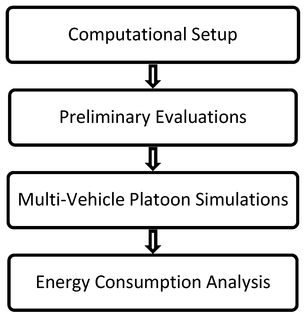
Figure 1 shows the overall approach of this study. Firstly, a computational fluid dynamics (CFD) model was developed in ANSYS FLUENT to simulate the aerodynamic flow around the vehicles in a platoon. Preliminary evaluations were then conducted on two-Ahmed body platoons to validate the computational setup. Next, single-vehicle simulations were conducted on the selected geometries of a passenger car and minibus to find an appropriate mesh size and to characterise the aerodynamic performance of the vehicles. The simulations were then extended to multi-vehicle platoons to analyse the influence of the number of vehicles, intervehicle distance and vehicle speed on the aerodynamic drag coefficients of the platoons. Lastly, using the drag coefficients obtained from CFD, the energy consumption of the vehicles in the platoons was calculated in a longitudinal dynamics simulation to evaluate the energy savings of the platoons.
In this study, two full-scale urban vehicle geometries were analysed to understand the effect of platooning. As displayed in
Figure 2, the vehicle geometries evaluated were a minibus known as the DART (Dynamic Autonomous Road Transit) model of dimensions 6.0 × 2.7 × 3.1 m developed by TUMCREATE, and a generic passenger car known as the DrivAer model of dimensions 4.6 × 1.7 × 1.4 m [
16] developed by TUM.
2.1. Computational Setup
The computational setup consisted of pre-processing the vehicle geometries, meshing, defining the fluid domain and finally assigning the appropriate boundary conditions to the model. Vehicle geometries were first simplified and defeatured in ANSYS SpaceClaim to remove small vehicle features that do not affect aerodynamic performance. Meshing and modelling the vehicles with these small features would otherwise result in a poor-quality mesh and a higher number of elements, resulting in computationally intensive simulations.
The vehicle geometries were then meshed in ANSYS Fluent meshing. Multiple refinement regions both at the front and the rear of each vehicle geometry, as shown in
Figure 3a,b, were defined to improve the accuracy of the incoming flow and wake regions at the front and rear regions, respectively. In addition, a parametric background mesh was created for the wind tunnel to allow for an increase in the domain length with the addition of vehicles in the platoon, as shown in
Figure 3c.
In ANSYS FLUENT, each vehicle and the background mesh were connected using the overset mesh interfaces. To minimise the pre-processing time for meshing, the overset meshing technique was adopted to be able to increase the number of vehicles and change the intervehicle distance in the fluid domain without needing to re-mesh the entire fluid domain repeatedly. Furthermore, only half the fluid domain was modelled, as the geometries of the vehicles were symmetric, and it was further assumed that the vehicles platoon exactly behind each other without any lateral offsets.
The steady state mass continuity and Reynolds-averaged Navier–Stokes (RANS) shown in Equations (1) and (2), respectively, were used to calculate the flow field. Where represents the mean and fluctuating components of the velocity in the three spatial directions (i = 1, 2, 3). is the pressure variable, is the density of the fluid, is the dynamic viscosity and the term represents the Reynolds stresses that are solved with a turbulence model using the Boussinesq hypothesis.
The realizable K-ε turbulence equations were used to model the turbulence in the fluid domain along with non-equilibrium wall functions to model the near-wall flow. The variables of the momentum (velocity), turbulence kinetic energy and turbulence dissipation rate were discretised using the second-order upwind scheme; the pressure variable was discretised using the second-order scheme; and the Least Squared Cell Based scheme was used to compute the gradient. A pressure-based coupled algorithm was used for the pressure–velocity coupling to iteratively solve the governing equations. All the simulations were conducted until the change in the drag coefficient of the platoon reduced below a value of 0.001.
The boundary conditions of the fluid domain are summarised in
Table 1. The inlet of the wind-tunnel zone was specified with a uniform velocity boundary equal to the vehicle speed. A pressure outlet condition was specified with zero-gauge pressure at the outlet surface of the wind tunnel. A stationary wall with a no-slip boundary condition was used for the vehicle body surfaces and the road surface. A symmetry boundary condition was used for the symmetrical plane of the vehicle body and wind tunnel. At the inlet, the turbulence intensity was specified to be 1% with a turbulence viscosity ratio of 10.
2.2. Preliminary Evaluations
Using the developed computational model, two-Ahmed body platoon simulations were first conducted to validate the computational setup and understand the aerodynamic behaviour of the platoon. Simulations were conducted for intervehicle distances between 0.25 and 3.0 m at a vehicle speed of 40 m/s. The results were then validated against the experimental studies from the literature [
11].
A mesh independence study was then conducted on the DART and DrivAer models to find an appropriate mesh size, taking both the accuracy and computational time into consideration.
Figure A1 in the appendix shows the results of the mesh independence study. The drag coefficient values reduced with the increase in mesh size until a mesh size of 4.8 million and 4.0 million cells for the DART and DrivAer vehicles, respectively; after which, there was no significant change to the drag coefficient value with a further increase in mesh size. The individual vehicles of the DART and DrivAer models were then simulated to obtain the isolated drag coefficient values of the respective vehicles. These values were then used as a baseline to evaluate the reduction in drag achieved through platooning.
2.3. Multi Vehicle Platoon Simulations
After the single-vehicle simulations, multi-vehicle platoons were analysed by increasing the number of vehicles in the fluid domain to 2, 3, 4, 5 and 7 as shown in
Table 2. The maximum number of vehicles in a platoon was limited to seven due to the operational constraints in urban environments. In addition to the number of vehicles in a platoon, different intervehicle distances and vehicle speeds were simulated. The intervehicle distances were varied with an interval of 1.0 m until the average platoon drag coefficient reached 95% of the isolated vehicle drag coefficient. Two vehicle speeds, 10 m/s (~36 km/h) and 30 m/s (108 km/h), were simulated, as the former represents the average speed of a vehicle and latter is the maximum speed limit in urban environments [
17]. In total, 70 different platoon combinations were analysed using the parameters shown in
Table 2.
2.4. Energy Consumption Analysis
The two driving cycles shown in
Figure 4 were used to simulate energy consumption. The BRT cycle (Bus rapid transit) [
18] which represents the speed profile for buses driving on dedicated lanes with signal priority is shown in
Figure 4a. The WLTP cycle (Worldwide harmonised light vehicles test procedure) [
19] which is the standard test cycle for light-duty vehicles is shown in
Figure 4b. To simulate the effect of platooning, it was assumed that the subsequent vehicles follow the driving cycle profiles with a constant headway as per their intervehicle distance. This assumption would hold for vehicles driving on dedicated lanes with traffic signal prioritisation.
Using the backwards simulation approach, the speed at each time step of the driving cycle was used to calculate the total driving resistance force in Equation (3). The total driving resistance force consists of the rolling resistance, acceleration, climbing and aerodynamic forces. The aerodynamic drag force was calculated using the drag coefficient, frontal area and vehicle speed, as shown in Equation (4). The values of the drag coefficient for the considered vehicles were obtained from the results of the computational analysis and interpolated based on speed, intervehicle distance and the vehicle′s position in the platoon i.e., lead vehicle, rear vehicle, etc.
where,
The total power consumption in Equation (5) was subsequently calculated based on the total driving resistance force, vehicle speed and the component efficiencies of the motor, inverter and transmission. The power consumption was then integrated over the duration of the driving cycle to obtain the energy consumption. The vehicle parameters of the two urban vehicles used in the longitudinal model are presented in
Table 3.
where,
For both the DrivAer and the DART vehicle platoons, the longitudinal simulations were repeated to obtain the energy consumption of each individual vehicle in the platoon based on the intervehicle distance and its position in the platoon. The mean energy consumption of the platoon was subsequently calculated and compared to the energy consumed by the isolated vehicle to obtain the energy savings due to platooning.
3. Results
To validate the computational setup, a two-Ahmed body platoon was first analysed.
Figure 5 shows a comparison of the simulated drag coefficient (body_CFD) of the front and rear Ahmed bodies to the experimental results (body_EXP) in [
11]. The simulated results show good agreement with the literature results for both the front and rear bodies. At intervehicle distances below 1 m, the drag coefficient of the front body reduced in comparison to the isolated value (isolated body), while that of the rear body increased. However, for intervehicle distances beyond 1 m, the values of the drag coefficient started to asymptotically converge to the isolated value for both the front and rear vehicles. The aerodynamic advantage of Ahmed body platooning was therefore only observed at intervehicle distances below 1 m.
After validating the computational setup, simulations were conducted for the isolated vehicles and subsequently for platoons of different sizes to obtain the drag coefficients of the vehicles. The simulation for the isolated vehicles resulted in a drag coefficient of 0.342 and 0.251 for the DART and DrivAer vehicles, respectively.
Figure 6 and
Figure 7 show the drag coefficient matrices of the DART and DrivAer platoons, respectively, at an intervehicle distance of 1 m and vehicle speed of 10 m/s. The drag coefficient values of the individual vehicles are represented with three different colours in the matrices. The vehicles that have a drag coefficient lower than the respective isolated value are denoted in green. The vehicles with a drag coefficient close to and higher than their isolated vehicle drag coefficients are denoted in yellow and orange, respectively.
From
Figure 6, it can be seen that the average drag coefficient of the two-vehicle DART platoon decreased by 23.4% in comparison to the isolated value. However, with an increase in platoon size to seven vehicles, the drag coefficient increased by 41.2% compared to the two-vehicle platoon. Moreover, the lead vehicles generally experienced a lower drag coefficient compared to the rear vehicles in the platoon. In some instances, however, the drag coefficient of the rear vehicles exceeded the isolated value. A similar trend was observed for intervehicle distances of 2, 3 and 4 m, as the lead and rear vehicles always resulted in the lowest and highest drag coefficients, respectively. This is shown in
Figure A2,
Figure A3 and
Figure A4 in the appendix.
For the DrivAer platoon, however, the average drag coefficient of the platoon reduced with the increase in platoon size, as shown in
Figure 7. The average drag coefficient for a seven-vehicle platoon reduced by 17% compared to the two-vehicle platoon at an intervehicle distance of 1 m. The trend in the drag coefficient of the individual vehicles in the platoon was, however, similar to the observations in the DART vehicle platoon. The lead vehicle had the lowest drag coefficient, while the rearmost vehicle had the highest drag coefficient. This trend can further be seen at intervehicle distances of 2 and 3 m, as shown in
Figure A5 and
Figure A6, respectively.
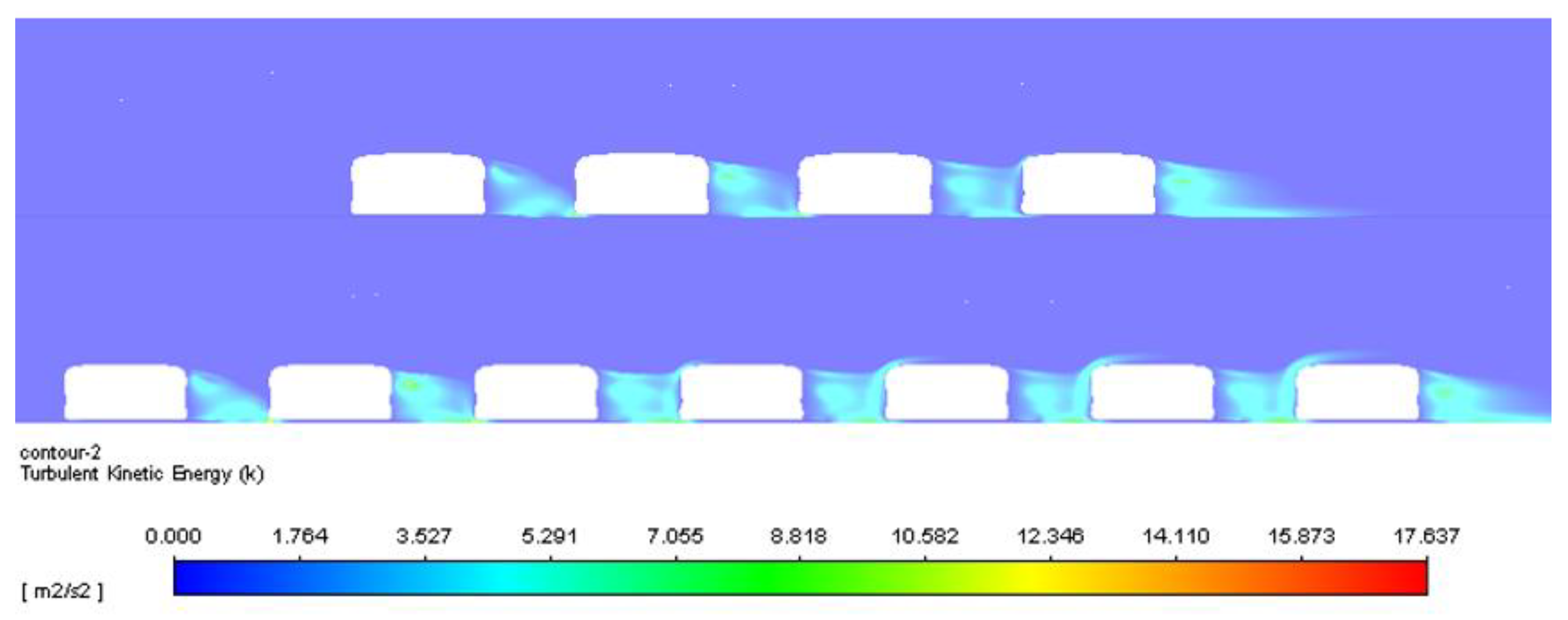
In addition to platoon size, the shape of the vehicle had a significant influence on flow characteristics and the resulting drag forces. As the DART vehicle design does not have a rear slant, the flow separation and vortex size are larger at the back surfaces of the vehicles leading to an increase in turbulence.
Figure 8 shows the Turbulence Kinetic Energy (TKE) contours of the DART vehicle platoon. With the addition of a vehicle in the flow field, the overall TKE increased at the back surfaces of the vehicles in comparison to the wake behind the first vehicle. This led to an increase in the turbulence of subsequent vehicles, thereby increasing the average drag coefficient of larger platoons of the DART vehicle. In addition, in comparison to
Figure 8 (top),
Figure 8 (bottom) shows an increase in the TKE region from the fifth vehicle as the turbulence extends to the top surfaces of the vehicles in the platoon.
On the other hand, the multi-vehicle DrivAer platoons did not exhibit any increase in turbulence in the wake of the downstream vehicle when compared with the wake of the upstream vehicles, as shown in
Figure 9. This difference in wake behaviour is due to the shape of the vehicle, as the DrivAer vehicle’s rear surface has a slant angle that prevents large separations of the flow resulting in a smaller wake. In contrast, the concave shape of the rear surface of the DART vehicle resulted in large flow separations and created a high degree of turbulence in the wake region.
For both the DART and DrivAer vehicles, the lead vehicle always resulted in the lowest drag coefficient and the last vehicle in the platoon generally had the highest drag coefficient. This is due to the separated flow from the lead vehicle which impinged on the front surface of the rear vehicle. The front surface of the rear vehicle therefore had a higher pressure coefficient, as shown in
Figure 10, for both the DART and DrivAer vehicles. The flow impingement on the rear vehicle enhanced the local pressure between the vehicles significantly and subsequently on the aft surfaces of the lead vehicle. As a result, the drag coefficient of the lead vehicle was reduced due to the decrease in the pressure difference between its front and aft surfaces.
The rear vehicle in the platoons, however, experienced the highest drag coefficient due to flow impingement which increased the frontal surface pressure and reduced the pressure on the aft surface due to the separation of the flow. The large pressure difference between the front and aft surfaces of the vehicle consequently increased the drag coefficient.
Subsequently, the influence of intervehicle distance on the average drag coefficient of the platoon was analysed for both vehicle geometries.
Figure 11a,b show how the normalised drag coefficient (as a percentage of the isolated vehicle drag coefficient) changed with intervehicle distance and platoon size for the DART and DrivAer platoons, respectively. Moreover, the error bars show the uncertainty in the simulation results (of ± 2.5%) due to grid discretisation and truncation errors.
Figure 11a shows that the normalised drag coefficient of the platoon increases with intervehicle distance. The drag coefficient of the two-vehicle DART platoon reduced by 23.4% at an intervehicle distance of 1 m but reduced by only 4% at an intervehicle distance of 4 m. This was because the average drag coefficient of the platoon seemed to approach the isolated value with the increase in the intervehicle distance. For larger platoon sizes, the aerodynamic advantage of platooning also reduced with the increase in intervehicle distance. The change in the drag coefficient value was, however, less prominent after an intervehicle distance of 2 m. Furthermore, the drag coefficient of the platoon exceeded that of the isolated vehicle for platoon sizes beyond four vehicles and intervehicle distances above 2 m.
For the DrivAer platoon, the normalised drag coefficient also increased with intervehicle distance and seemed to approach the isolated value, as shown in
Figure 11b. The normalised drag coefficient increased from 91% to 96% with the change in the intervehicle distance from 1 to 3 m, respectively. However, for larger platoon sizes, the magnitude of the change in the drag coefficient with the intervehicle distance was higher, as the normalised drag coefficient for a seven-vehicle platoon increased from 76% to 94% with the change in intervehicle distance from 1 to 3 m, respectively.
The influence of vehicle speed on the drag coefficient of the vehicles and platoon was analysed for speeds of 10 and 30 m/s for both the DrivAer and DART vehicles. The change in vehicle speed influenced flow characteristics such as the size of the wake at the rear of the vehicles, the flow impingement at the front surfaces and the turbulence intensity of the flow, thereby affecting the drag coefficient of the vehicles in the platoon. However, the results show that vehicle speed did not significantly influence the drag coefficient of the vehicles in the platoon.
Table 4 summarises the results from the simulation. As the speed changed from 10 to 30 m/s, the percentage change in the drag coefficient varied between −1.28% and 3.94%. No correlation was found between the vehicle speed and the drag coefficient at different intervehicle distances and platoon sizes.
Lastly, the energy consumption and subsequent energy savings due to platooning were analysed for different intervehicle distances and numbers of vehicles.
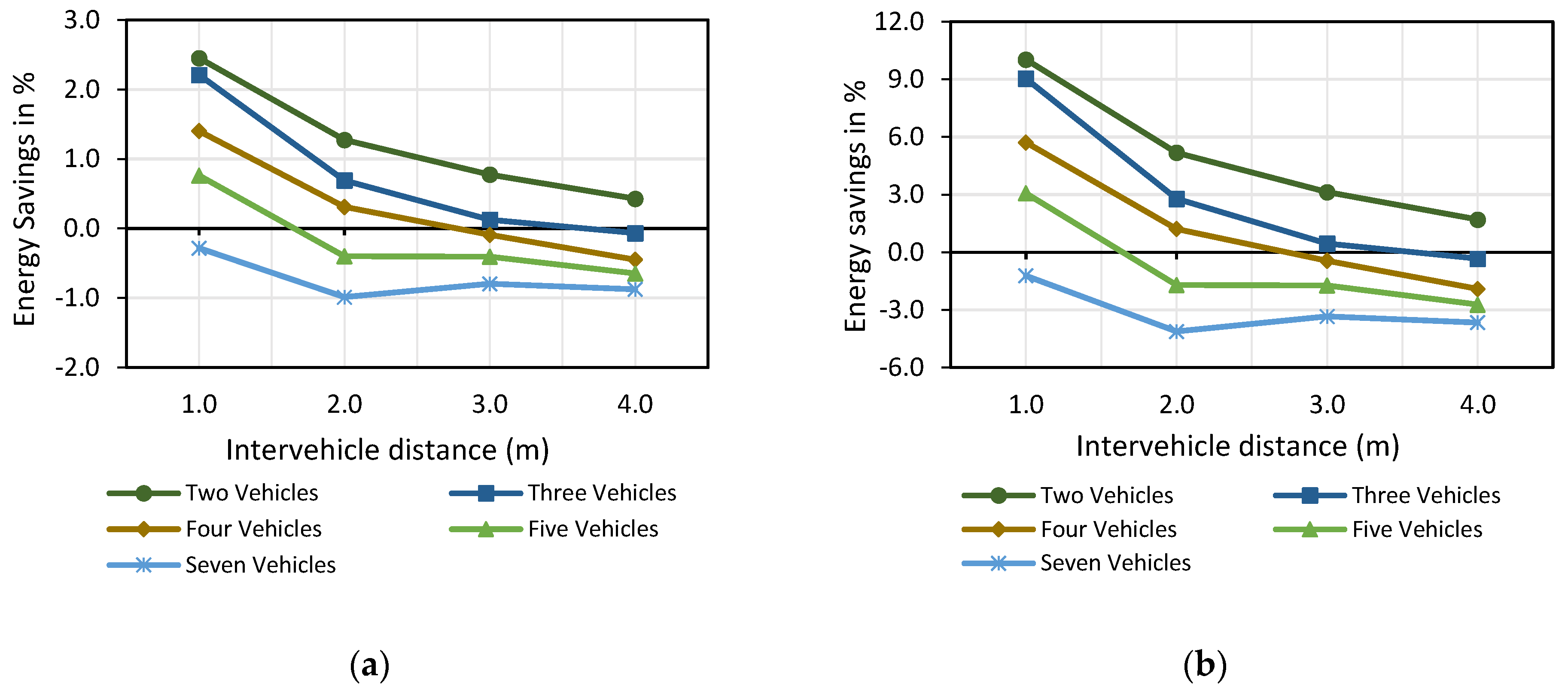
Figure 12a,b show the overall energy savings of the DART vehicle platoon for the BRT and WLTP driving cycles, respectively, in comparison to the energy consumption of the isolated vehicle. The results show that an increase in intervehicle distance or platoon size reduced the overall energy savings for the DART vehicle platoons. This trend was more visible for the platoons with a smaller number of vehicles, i.e., less than five vehicles. For platoon sizes larger than five vehicles, the average energy consumed by the vehicles in the platoon exceeded that of the isolated vehicle.
Although both the driving cycles exhibited a similar trend in energy savings with changes in platoon size and intervehicle distance, the WLTP cycle resulted in higher energy savings of 10%, in comparison to 2.5% for the BRT cycle for a two-vehicle platoon at 1 m. The energy savings, however, reduced to 0.4% and 1.7% for the BRT and WLTP cycles, respectively, when the intervehicle distance was increased to 4 m. Furthermore, as the platoon size increased to seven vehicles, the average energy consumed by the platoon exceeded the isolated value by 0.9% in the BRT cycle and 3.6% with the WLTP cycle at an intervehicle distance of 4 m.
The WLTP cycle had higher energy savings due to the higher average speed of 54 km/h (13 m/s) in comparison to the BRT cycle with an average speed of 22 km/h (6 m/s). This is because the reduction in the drag forces with platooning was more pronounced at higher vehicle speeds due to the quadratic increase in aerodynamic drag forces.
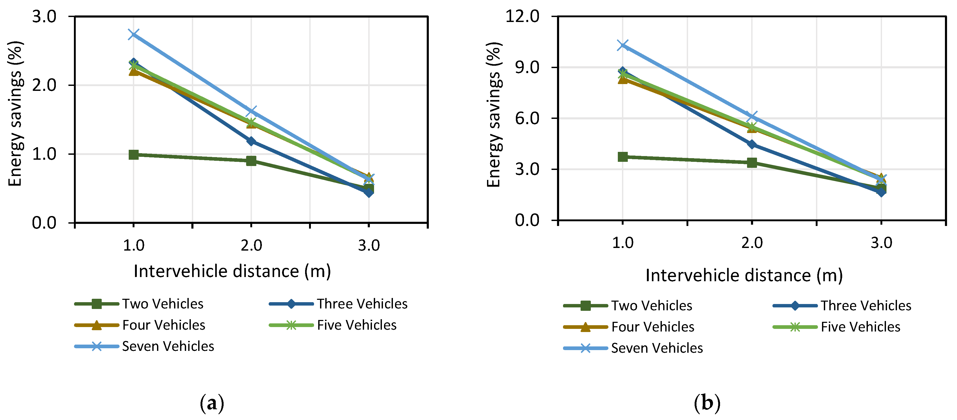
On the contrary, as shown in
Figure 13a,b, increasing the number of vehicles to seven in the DrivAer platoon resulted in higher energy savings of 2.7% for the BRT cycle and 10.3% for the WLTP cycle at an intervehicle distance of 1 m. However, at an intervehicle distance of 3 m, the energy savings of the platoon decreased to 0.6% and 2.4% for the BRT and WLTP cycles, respectively. For the DrivAer vehicles, platooning is therefore more beneficial for platoon sizes greater than two vehicles and at intervehicle distances less than 3 m.
4. Conclusions
In this paper, we computationally analysed two vehicle concepts to understand the aerodynamic drag behaviour and subsequent changes in energy consumption of autonomous electric vehicle platoons in urban environments. A CFD analysis was conducted on two vehicle geometries: a minibus–DART and a passenger car model–DrivAer. The influence of intervehicle distance, platoon size and vehicle speed on the drag coefficient of the platoons was investigated. Finally, a longitudinal dynamics simulation was conducted to assess the resulting effect of changes in the drag coefficient on the average energy consumption of the platoons.
The results for the DART vehicle platoons showed a reduction in the average drag coefficient by up to 23% and subsequent energy savings of 2.5% and 10% for the BRT and WLTP cycles, respectively. However, with the increase in intervehicle distance, the aerodynamic advantage of platooning reduced. It was further found that the increase in platoon size adversely affected the aerodynamic performance of the platoon, as the average drag coefficient exceeded that of a single DART vehicle in isolation for a platoon size of seven vehicles. Platooning is therefore less aerodynamically beneficial for DART vehicles when the platoon size is greater than three vehicles or at large intervehicle distances exceeding 4 m.
For the DrivAer vehicle, the results showed that an increase in the platoon size reduced the average drag coefficient of the platoon. For a seven-vehicle platoon at 1 m, the drag coefficient of the platoon decreased to 24% with corresponding energy savings of 2.7% and 10.3% for the BRT and WLTP cycles, respectively. However, as the intervehicle distance increased to 3 m, the average drag coefficient reduced by only 6% of the isolated value with energy savings of 0.6% and 2.4% for the BRT and WLTP cycles, respectively. Platooning for the DrivAer vehicle was therefore found to be more advantageous for platoon sizes greater than two vehicles or at intervehicle distances below 3 m. For intervehicle distances exceeding 3 m, the average drag coefficient of the platoon approached the isolated value thereby not resulting in significant energy savings.
Furthermore, it was found that the shape of the vehicle had a large influence on the drag coefficient of the vehicles. The drag coefficient of the DART vehicle platoons increased with the number of vehicles in the platoon, while that of the DrivAer vehicle platoons decreased. This was largely due to the wake structure and the separation of the flow at the rear and top surfaces of the vehicles, which adversely affected the flow ahead of subsequent vehicles. The shape of the vehicle should therefore be optimised to take advantage of platooning.
Vehicle speed did not strongly influence the drag coefficient but largely affected the energy consumption of the vehicles due to the quadratic increase in the aerodynamic forces at higher speeds. The WLTP cycle was therefore found to benefit more from platooning than the BRT cycle due to its higher average speed.
This study did not consider the safety aspects of platooning. In practice, it may be very challenging for vehicles to platoon at intervehicle distances below 4 m at higher vehicle speeds. The energy savings would therefore be lower if vehicles cannot platoon at smaller intervehicle distances. Furthermore, this study assumed a constant headway between the vehicles in a platoon when calculating the energy consumption. In practice, the intervehicle distances between the vehicles would change while driving and during different phases of acceleration and deceleration. This would also influence the energy consumption of the vehicles in a platoon and would need to be considered in detail. The results of the drag coefficient obtained from the CFD analysis can be further used in speed trajectory optimisations and control of autonomous platoons to determine and optimise the total energy consumption of the platoons.


