End-Point Model for Optimization of Multilateral Well Placement in Hydrocarbon Field Developments

Abstract

Drilling cost is one of the most critical aspects in the reservoir management plan. Costs may exceed a million dollars; thus, optimal designing of the well trajectory in the reservoir and completion are essential. The implementation of a multilateral well (MLW) in reservoir management has great potential to optimize oil production. The object of this study is to develop an integrated workflow of end-point multilateral well placement optimization integrated with the reservoir simulator supported by artificial intelligence (AI) methods. The paper covers various types of MLW construction, including: horizontal, bi-, tri-, and quad-lateral wells. For quad-lateral wells, the capital expenditure is highest; nevertheless, acceleration of oil production affects the project’s NPV (net present value), indicating the type of well that is most promising to implement in the reservoir. Tri- and quad-lateral wells can operate for 12.1 and 9.8 years with a constant production rate. The decreasing hydrocarbon production rate is affected by reservoir pressure and the reservoir water production rate. Other well design patterns can accelerate water production. The well’s optimal trajectory was evaluated by the genetic algorithm (GA) and particle swarm optimization (PSO). The major difference between the GA and PSO optimization runs is visible with respect to water production and is related to the modification of one well branch trajectory in a reservoir. The proposed methodology has the advantage of easy implementation in a closed-loop optimization system coupled with numerical reservoir simulation. The paper covers the solution background, an implementation example, and the model limitations.

1. Introduction

We provide a state-of-the-art background and place the proposed approach among other solutions. The Introduction consists of a review of the application of multilateral well system in various production and injection scenarios, a review of previous works related to multilateral well optimization, a brief description of the optimization algorithms that can be employed in the solution with special consideration of the genetic algorithm and particle swarm optimization.

1.1. Multilateral Wells as an Asset in Reservoir Management

In recent years, the interest in multilateral wells has increased. The advanced technologies for the completion of productive horizons using multilateral or intelligent wells offer several possibilities to optimize hydrocarbon recovery and economic results [1]. The biggest advantages of multilateral wells are the increased formation drainage area and enhancement of productivity. This technology brings the benefits of reducing water cresting and coning due to complex structured branch wells usually having a higher production rate with a smaller production pressure difference compared to a vertical or single horizontal well [2]. Therefore, it helps to significantly postpone water breakthrough especially in reservoirs with a strong bottom water drive mechanism. Additionally, the technology of multilateral wells can considerably decrease capital expenditures in the field development phase, owing to a large part of the costs being incurred when drilling the main hole [3], in that one multilateral well can replace multiple vertical or horizontal wells in overall production and recovery [4]. Currently, most offshore wells start vertically, but they typically contain numerous out-of-plane horizontal or dipping drain holes whose flow areas interact [5]. Designing the trajectory, quantity, and placement of lateral wells from one mainbore requires a detailed analysis of the reservoir and fluid that will be produced. The optimal placement may bring high gas or oil recovery and substantial profits to the investment, but finding the best solution for the objective function is extremely challenging and involves plenty of variables. Among the factors that can affect overall reservoir performance and project profitability, several major groups emerge. Petroleum fluids, reservoir rock properties, and management schema contribute to the oil recovery and its production [6]. As an example of the physical phenomena affecting production performance, multiphase flow, oil-aqueous interfacial tension, and the contact angle between phases can be listed. Furthermore, fluid properties and pressure-temperature changes can play a major role in recovery [7]. Song et al. [8] introduced a novel method of the utilization of multilateral wells in the oil shale in situ conversion process. The proposed method employs radial branches from the main trunk in the upper and lower oil shale formation as injection and production points. Due to the temperatures of the injected fluid to initiate the pyrolization process, the authors performed a sensitivity analysis to evaluate the impact of the oil properties and the arrangements of radial branches’ placement. One of the crucial parameters that has a significant impact on multilateral well performance is pressure drop in the horizontal part. Wei et al. [9] developed a semi-analytical model to investigate the pressure drop within a multilateral horizontal well. The proposed model covers a wide range of flow regimes. Model verification was conducted on the two most common well patterns. Apart from the application of a multilateral well in a conventional reservoir production system, a multilateral well (MLW) can be used in coalbed methane, heavy oil, or geothermal systems. Yang et al. [10] analyzed CMB (coal bed methane) occurrence and the multilateral horizontal well trajectory in the Qinshui Basin, Shanxi Province. The investigation made an effort to provide a solution to the problem of slack coal production in gas recovery by reduction of the permeability due to water saturation. Chen et al. [11] investigated the characteristics of coal permeability anisotropy and its impact on the optimal multilateral well design. The results showed that the optimal well direction of the quad-lateral well is parallel to the cleat. However, stress changes during the production period may also have a significant impact on multilateral well design. Zhou et al. [12] proposed an investigation of the limits of sand production from offshore heavy oil reservoirs through laboratory experiments and a numerical simulation. The obtained results suggested the number of branches be limited to two or three, taking into account the design parameters, especially the branch angle. Shi et al. [13] evaluated the possibility of increasing the heat extraction from CO₂ enhanced geothermal systems (CO₂-EGS) by the application a multilateral well system. The authors used a coupled wellbore–reservoir model with fluid flow and heat transfer. The multilateral well construction was optimized to achieve the maximum heat insulation. The results provided suggestions for the wellbore design pattern. According to [14], the most efficient way to maximize hydrocarbon recovery is long directional wells. The author gave as an example the Troll field, one of the biggest oil and gas fields in the North Sea in Norway, which is made up of huge and thin reservoirs. This field deployed multilateral wells with horizontal lengths up to 5.5 km. Moreover, the wells are equipped with intelligent control devices that help to maintain uniform inflow rates across the entire length of the interval and delay water or gas breakthrough. This makes them very useful and important from a production perspective.

1.2. State-Of-The-Art in Multilateral Well Placement Optimization

Many studies propose different methods for the optimization of multilateral well design, and each of them takes into account different aspects. Lyu et al. presented a semi-analytical method for a multilateral well design, which was based on the drainage area [15]. The objective function was to exploit the entire reservoir as efficiently as possible within a certain time. The proposed algorithm can determine the number of lateral wells, the lateral length, and the spacing of the lateral wells. The advantages of the method are that it is applicable to different types of reservoirs and the computation time is short. However, to represent the heterogeneity of the reservoir, it uses only a 2D model of the geological properties. You et al. proposed a model that enables estimating the water breakthrough time and breakthrough locations in multilateral horizontal wells [2]. The method is mainly applicable to bottom water-drive reservoirs. A properly designed well can substantially delay the water breakthrough time, resulting in extend production time and hydrocarbon recovery. The model proposed by You et al. considered many factors, including the well trajectory (distance between the wellbore and bottom boundary, main wellbore length, each branch’s well length), wellbore vertical location, reservoir and fluid properties (oil viscosity and density, formation water density), as well as petrophysical properties (formation isotropic permeability). Lyu et al. proposed the multilateral well trajectory and configuration optimization method for fractured reservoirs based on the connectivity ratio [16]. They employed a fast marching method. The objective function was to maximize the ratio between the total length of effectively connected fractures to the well, granted that greater penetration of the fractures improves the productivity of the well. The proposed method optimizes the well trajectory taking into account the geological properties, but does not consider such factors as the fluid flow in fractures and matrix and stress sensitivity. Only the azimuths of lateral wells are determined without an inclination angle. The proposed model is very fast even for complex reservoirs. Currently, artificial intelligence (AI) with different techniques (such as neural networks, fuzzy logic, the genetic algorithm, particle swarm algorithm, etc.) is used broadly in many disciplines including the oil and gas industry. These methods imitate intelligent human behavior in solving engineering problems related to prediction, drawing conclusions, and actions. In a complex task with multiple variables, it is difficult to find an optimal solution employing analytical methods due to the lack of direct dependency between individual variables, the objective function, and the constraints [1]. AI methods have been worked out in optimization tasks, as well as in predicting various parameters associated with high uncertainties. Buhulaigah et al. [17] in their study compared the analytical model using Borisov’s correlation with the artificial neural network (ANN) approach to predict the average oil flow rate of multilateral wells. The obtained results indicated the great accuracy and advantage of AI methods over analytical ones. ANN gave a forecast error of 7.85% against actual rates compared to the 50.4% calculated from Borisov’s correlation. Among AI techniques, the expert system plays a crucial role in combining expert knowledge with self-learning algorithms. Garrouch et al. [18] introduced a web-based fuzzy expert system for preliminary planning and completion of a multilateral well.

1.3. Genetic Algorithm and Particle Swarm Optimization Procedure

The necessities of the continuity and differentiability of the objective function significantly limit the possibility of using the application of gradient methods in real optimization problems. Therefore, a number of optimization methods were developed and implemented, which were aggregated according to the common name for evolutionary methods, which are inspired by biological analogies, mainly natural evolution. Contrary to gradient methods, they are based on a single solution; evolutionary methods are based on a certain set of solutions (populations of individual solutions). Evolutionary methods assume that the solution population changes to fit the optimization problem, creating a new population. The individual solution is assessed in terms of the quality of the objective function, and on this basis, the probability of the transition to a new population (survival) is given. Solutions with a worse quality are abandoned during the algorithm’s operation. Evolutionary methods only require that an objective function value be assigned to each individual solution. This enables the use of a reservoir simulator, which can act as a black box, calculating the value of the objective function for a given vector of decision variables. Among evolutionary algorithms, the genetic algorithm (GA) and particle swarm optimization (PSO) techniques have been the most intensively studied during the last few years. In this paper, the genetic algorithm is chosen as an industrial standard procedure for optimization, and PSO is selected as the second algorithm for solution comparison.

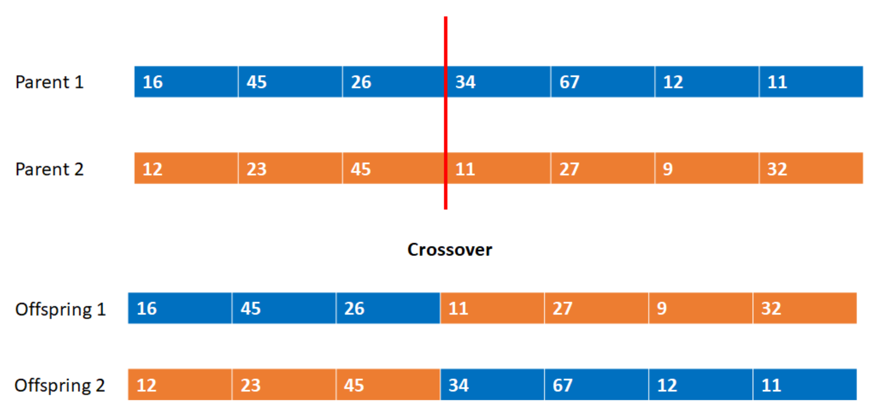
1.3.1. Genetic Algorithm

GA is a search-based optimization technique based on the principles of natural selection. It is used to find optimal or near-optimal solutions to difficult problems. The terminology used to describe the genetic algorithm is derived directly from biological nomenclature. Each potential solution to an optimization problem is named as an individual (chromosome). The essential step of each iteration of the algorithm is to calculate the matching of individuals included in the population by calculating the corresponding value of the objective function. Fit is a measure showing the effectiveness of a solution by a given individual. During a GA run, the parental population is selected. Individuals making up this pool are subjected to crossover and mutation, leading to the creation of a descendant population [19]. The selection of the parental population is most often made on the basis of a single tournament method [20,21]. It consists of dividing the population into small subsets, usually composed of several individuals. From each group, a pair of individuals with the highest matching is selected to be the parents of the child solution. The best-matched individual in each iteration can have at most one descendant, which prevents premature convergence of the algorithm. The genetic algorithm is based on characteristic operators. The role of the crossover operator is to exchange information between the parents, with a certain probability of obtaining offspring representing a better quality match. The crossover operator is based on a random selection of the intersection of the chromosome chains. The first offspring is made by copying the first part of the parent’s genes to the cut point, and the rest are selected from the second parent, as presented in Figure 1.

The second offspring is created in an analogous manner from the rest of the parents’ genes. Mutation operators turn a chromosome into a different chromosome. The essence of the crossover operator is the exchange of information between individuals, while the role of mutation is to introduce small random changes in individuals, as presented in Figure 2.

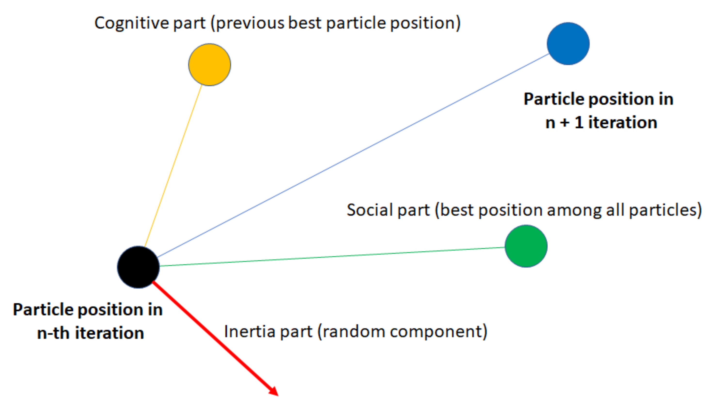
1.3.2. Particle Swarm Optimization

Particle swarm optimization is a stochastic population-based optimization method proposed by Eberhardt and Kennedy [22,23]. The algorithm mimics social swarm behavior where, while gaining experience, particles interact with each other and exchange information, moving to better areas of the solution space, thus striving for the global optimum [24]. In each iteration, each particle representing an individual solution moves in the solution space with a certain speed (speed as a change in the position of the particles in the solution space for a certain number of iterations performed, where the position should be notified as the location of the vector of decision variables in the search space). It follows that the particle representing the vector of decision variables moves in n-dimensional space, as shown in Figure 3.

PSO’s principles are based on the exchange of information about the location of a better quality area in the solution space between adjacent particles.

1.4. The Article’s Objective

Multilateral wells are concerned as a requirement in the effective management of hydrocarbon reservoirs, especially in off-shore applications; thus, the optimization of the trajectory planning should be taken into consideration. The paper aims to develop a methodology for a multilateral well pattern for any number of branches’ end-point conjunction with a numerical simulator and optimization algorithm to provide the optimal well topology in the reservoir management system.

2. Methodology

In connection with the growing interest in multilateral wells in oil and gas reservoir management, the enhanced optimization model is presented. The modeling of multilateral wells is based on the division of trajectories into nodal points and segments that are assigned to blocks of the simulation model, as presented in Figure 4.

2.1. End-Point Multilateral Well Model

In this section, the details of the optimization workflow will be presented. The end-point model workflow will be introduced, and the implementation example will be demonstrated.

2.1.1. Workflow

The end-point multilateral well optimization model is based on the reservoir numerical simulator. The basic principles require dividing the reservoir into a series of cells. Each cell of the reservoir model has discrete coordinates $\mathit{s}$ related to the block center point, as presented in Figure 5.

$$\mathit{s}=\left[\begin{array}{ccc}{s}^{\left(x\right)}& s^{\left(y\right)}& s^{\left(z\right)}\end{array}\right]$$

(1)

where $s^{\left(x\right)}$, $s^{\left(y\right)}$, $s^{\left(z\right)}$ are the spatial coordinates of the reservoir model cell in the x, y, z directions, respectively. Thus, the simulation model domain $\mathrm{\Omega }$ can be expressed as a set of reservoir blocks:

$$\mathrm{\Omega }=\{{\mathit{s}}_1,{\mathit{s}}_2,\dots ,{\mathit{s}}_N\}$$

(2)

where N is the total cell number in the reservoir model.

The implementation of the end-point model requires a numerical model with orthogonal cells. The following steps are necessary to obtain the input to the numerical simulation:

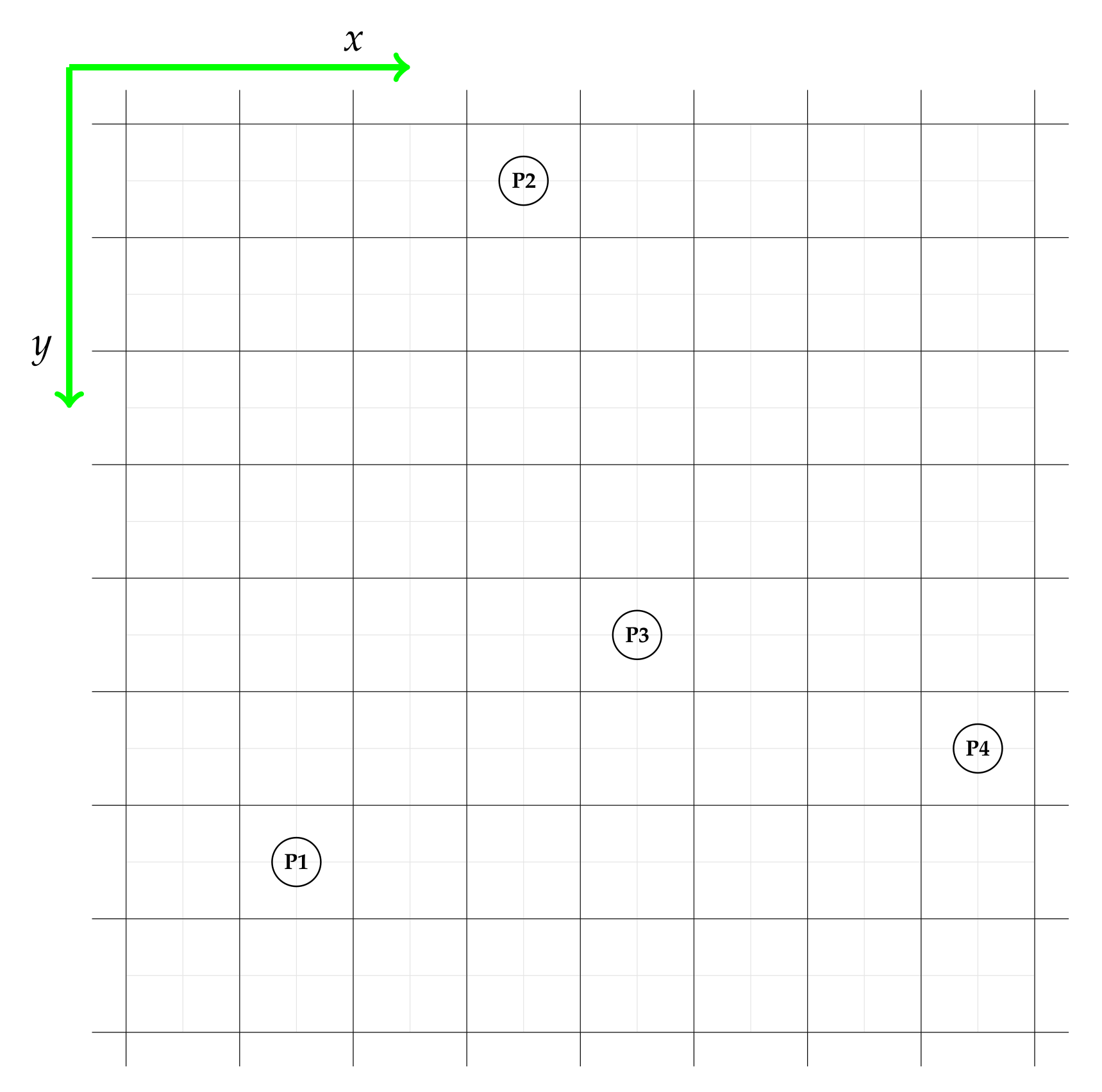
• Create end-point well set $\mathit{P}$ by picking $N_g$ points (where $N_g\ge 2$) from the reservoir domain $\mathrm{\Omega }$, where $N_g$ numbers of total end-points are determined (Figure 6):

  $$\mathit{P}=\{{\mathit{s}}_1,\dots ,{\mathit{s}}_{N_g}\},\mathit{P}\in \mathrm{\Omega }$$

  (3)
• Due to the well construction assumption, the total number of lateral wells (branches) is equal to $N_g-1$, meaning that for a horizontal well (one branch), $N_g=2$ is required; for a bi-lateral well, $N_g=3$ is mandatory, etc.;
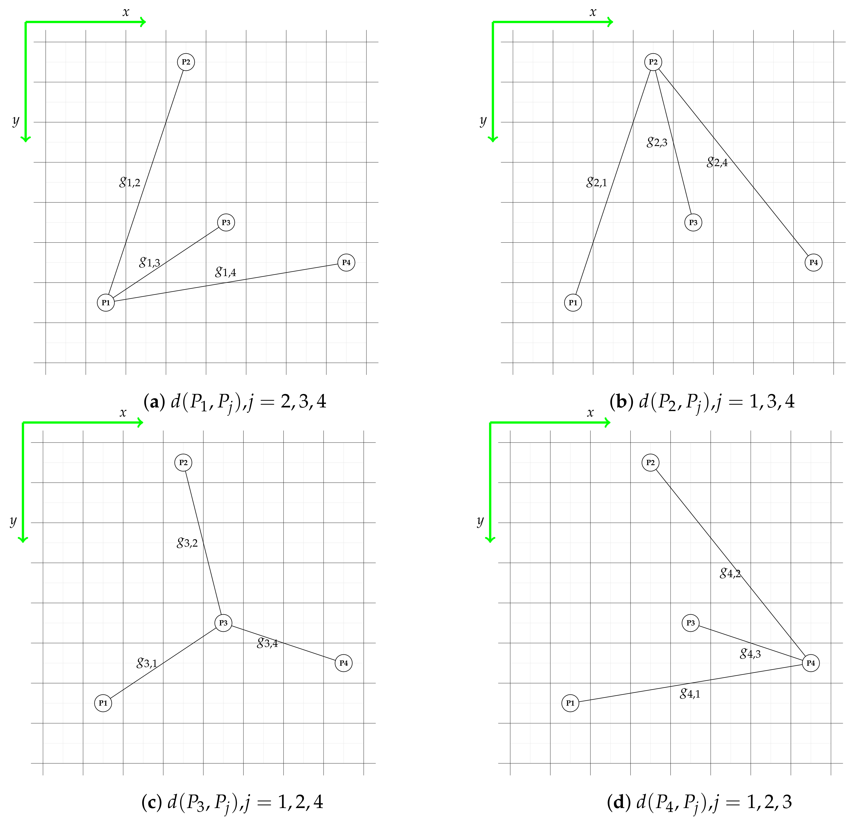
• Individual branch $g_{i,j}$ is represented by the section connected at the junction point: ${\mathit{P}}_i\to {\mathit{P}}_j$; thus, we elaborate all possible connections between points in the set (Figure 7 represents the connection possibilities depending on the central point);
• The end-point well optimization algorithm focuses on minimizing the total branches’ lengths $|{\sum }_{i=1}^{N_g-1}{g}_i|\to min$. In other words, we want to find such a point-to-point connection pattern that minimizes the sum of the branches’ lengths. In this manner, the central point has to determine $\check{\mathit{P}}$;
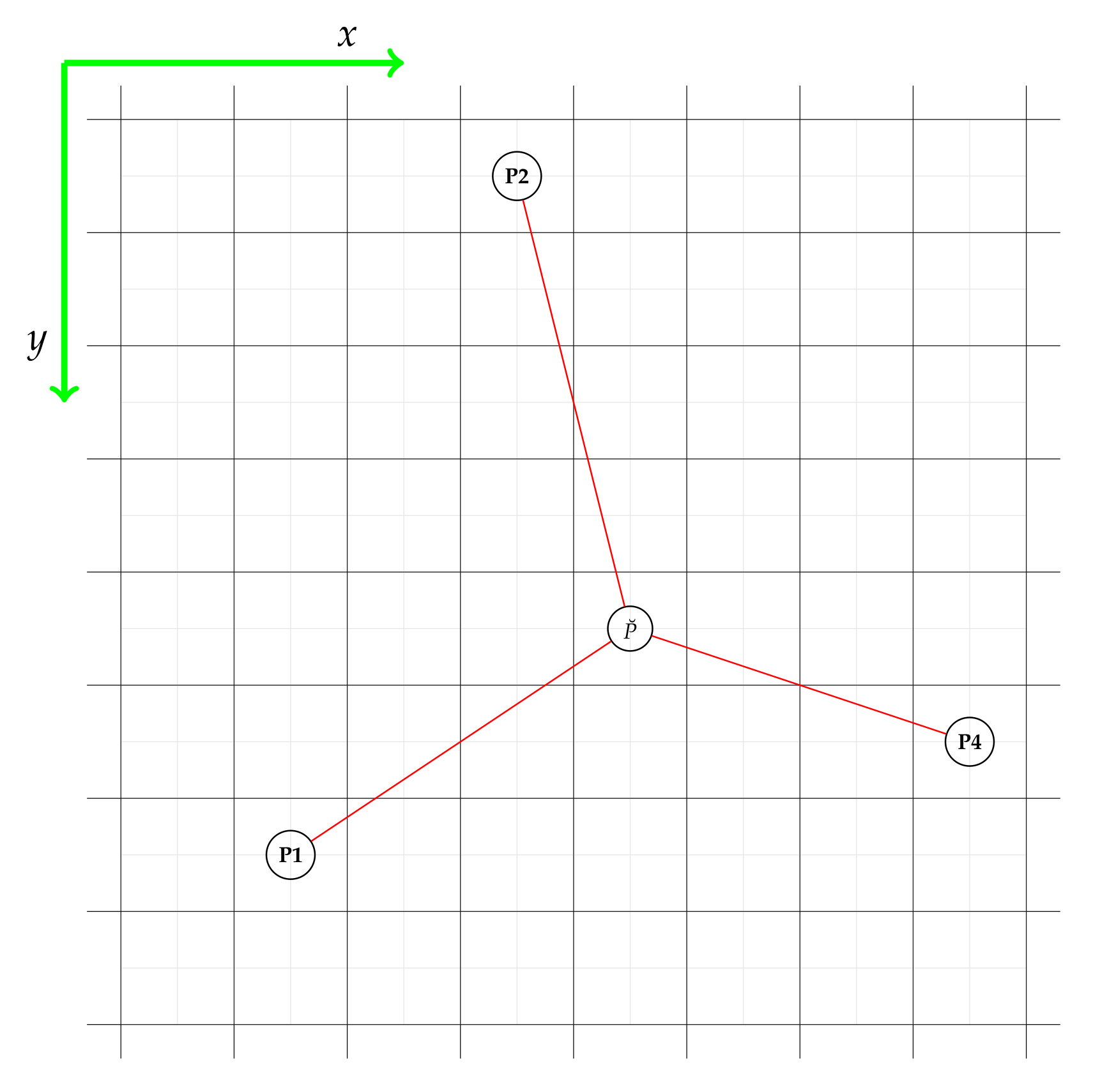
• In end-point well set $\mathit{P}$, get the central point (well trunk) $\check{\mathit{P}}$ fulfilling the following assumption of the minimizing total branch length:

  $$\check{\mathit{P}}={\mathit{P}}_k,\mathrm{where}:k=\mathrm{argmin}\sum _{i,j=1}^{N_g}d\left({\mathit{P}}_i,{\mathit{P}}_j\right)$$

  (4)

  where the distance between each point in the set is calculated by the following equation:

  $$d\left({\mathit{P}}_i,{\mathit{P}}_j\right)=\sum _{i,j=1}^{N_g}\sqrt{\sum _{n=1}^3{\left({\mathit{s}}_i^n-{\mathit{s}}_j^n\right)}^2},i,j\in \{1,\dots ,N_g\},n\in \{x,y,z\},i\ne j$$

  (5)

  and argmin is a function returning the index of the point:

  $$\underset{\mathit{P}}{\mathrm{argmin}}\sum _{i,j=1}^{N_g}d({\mathit{P}}_i,{\mathit{P}}_j)=\{\breve{\mathit{P}}\in \mathrm{\Omega }\wedge \forall \mathit{P}\in \mathrm{\Omega }:d(\breve{\mathit{P}},{\mathit{P}}_j)=\min d({\mathit{P}}_i,{\mathit{P}}_j)\}$$

  (6)
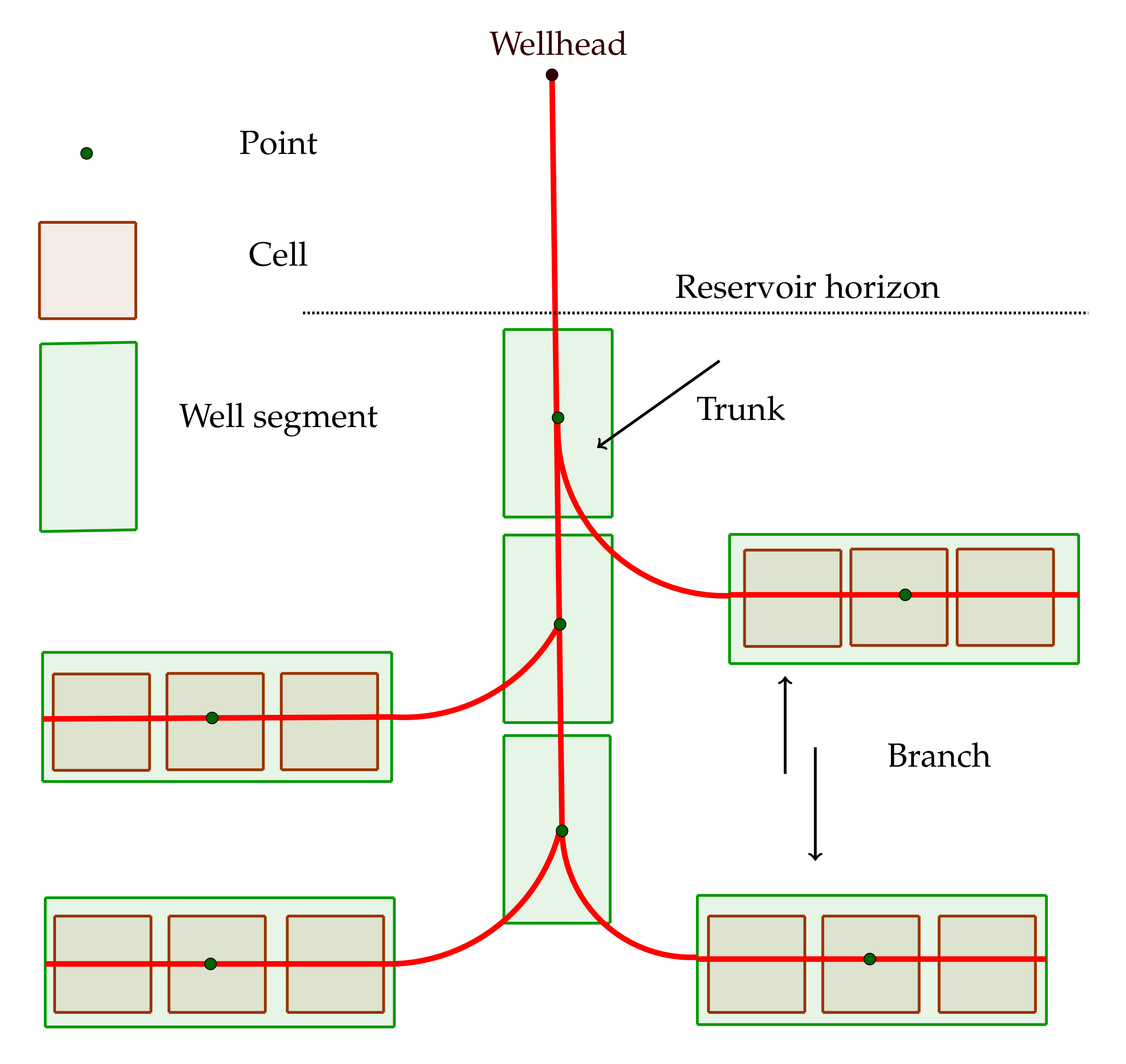
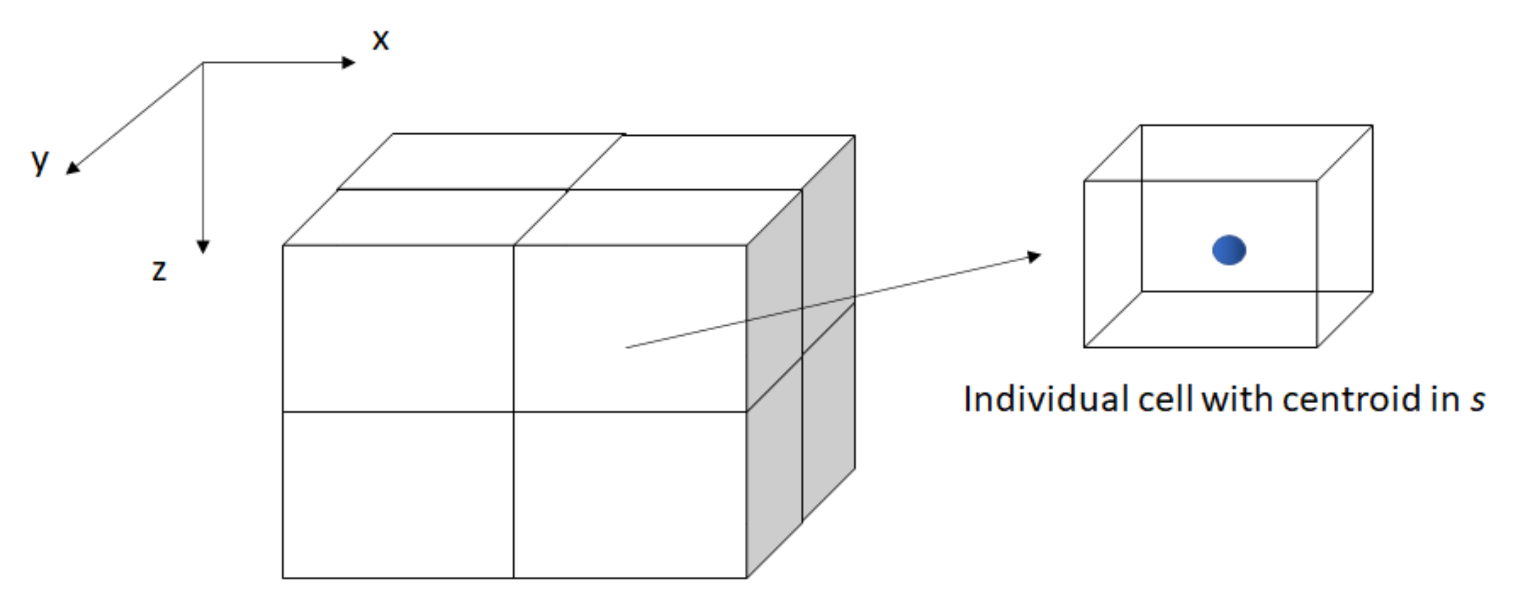
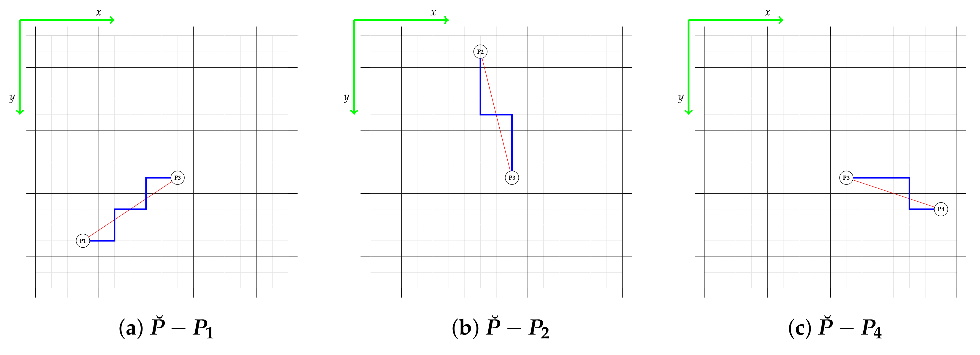
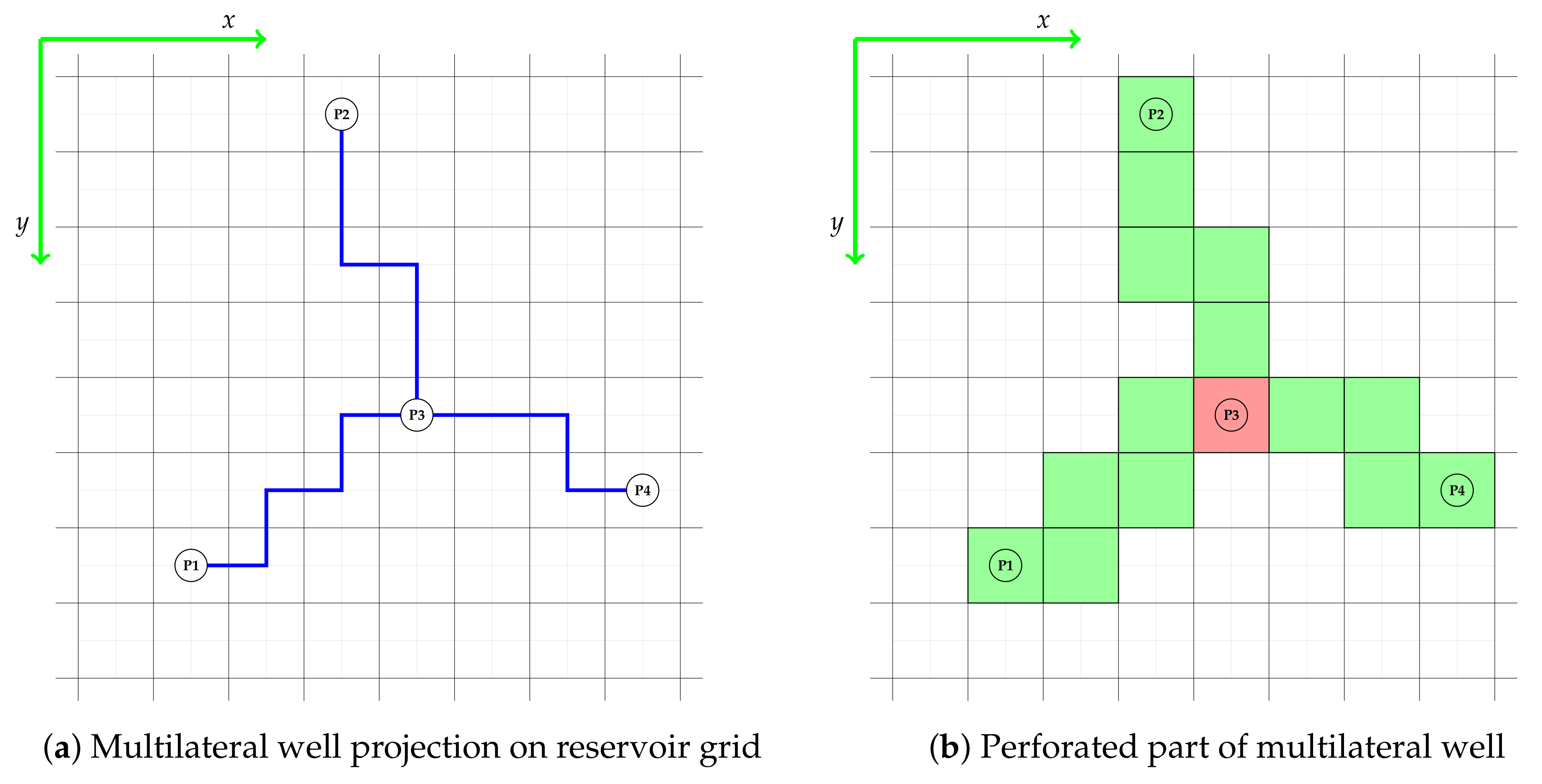
• The reservoir simulation used in this study (Schlumberger Eclipse, version: 2019a Manufacturer: Schlumberger) requires discrete approximation of the well trajectory; thus, the trajectory of the well must be approximated to a center point block of the simulation grid. Branch matrix $\mathit{U}$ contains the well trajectory:

  $$\mathit{U}=\left[\begin{array}{ccc}\check{s^{\left(x\right)}}& \check{s^{\left(y\right)}}& \check{s^{\left(z\right)}}\\ s_{1,1}^{\left(x\right)}& s_{1,1}^{\left(y\right)}& s_{1,1}^{\left(z\right)}\\ s_{1,2}^{\left(x\right)}& s_{1,2}^{\left(y\right)}& s_{1,2}^{\left(z\right)}\\ ⋮& ⋮& ⋮\end{array}\right]\begin{array}{c}\to \mathrm{Trunk}\\ \to \mathrm{first}\mathrm{branch},\mathrm{first}\mathrm{node}\\ \to \mathrm{first}\mathrm{branch},\sec \mathrm{ond}\mathrm{node}\\ ⋮\end{array}$$

  (7)
• The common part of individual trajectories can be written as a set of points with coordinates $\left(s^{\left(x\right)},s^{\left(y\right)},s^{\left(z\right)}\right)$, which belong to both the side branch ${\mathit{U}}_k$ and branch ${\mathit{U}}_l$:

  $$\begin{array}{cc}\hfill {\mathit{U}}_k\cap {\mathit{U}}_l=& \left\{\{s^{\left(x\right)},s^{\left(y\right)},s^{\left(z\right)}\}:\{s^{\left(x\right)},s^{\left(y\right)},s^{\left(z\right)}\}\in g_k\wedge \{s^{\left(x\right)},s^{\left(y\right)},s^{\left(z\right)}\}\in g_l\right\},\hfill \\ \hfill & k\ne l,k,l\in \left\{1,\dots ,N_g-1\right\}\hfill \end{array}$$

  (8)
• The analysis of the mutual part of the lateral well trajectory allows determining which cells should be treated as open (perforated) according to the algorithm, because multiple connections in the same cell are forbidden:

  $$P_{f_a}=\left\{\begin{array}{ccc}0& \mathrm{if}& {\mathit{U}}_k\cap {\mathit{U}}_l\ne \mathsf{Ø}\\ 1& \mathrm{if}& {\mathit{U}}_k\cap {\mathit{U}}_l=\mathsf{Ø}\end{array}\right.,a\in \mathsf{\Omega }$$

  (9)
• Cells marked with the index $P_{f_a}=1$ are treated as open, while those with index $P_{f_a}=0$ are closed for the well. The following assumptions allow avoiding sharing the same block by different side wells.
• The perforation matrix is translated to the simulator keyword and is included in the simulation run.

2.1.2. Implementation Example

An example implementation of the node search $\check{\mathit{P}}$ is presented in Figure 6, Figure 7, Figure 8 and Figure 9. It was assumed that the trajectory of the well would run in one plane of the model ($s^{\left(z\right)}=const.$). The construction of the well trajectory will be based on $N_g=4$ nodal points, which will lead to the creation of a planar tri-lateral well.

The center nodal point ($\check{\mathit{P}}$) search is based on calculating the length of the branches for all possible combinations of point connections, as shown in Figure 7.

Based on the argmin function evaluation, central nodal point $\check{\mathit{P}}$ is set as ${\mathit{P}}_3$. As in the case of vertical wells, the actual trajectory of the well must be approximated to a center point block of the simulation grid. An example of the trajectory approximation on a numerical grid is shown in Figure 8 and Figure 9. As a result of the approximation, we get the $\mathit{U}$ trajectory matrix containing individual branch trajectories, which are described by the points $\left[\begin{array}{ccc}{s}^{\left(x\right)}& s^{\left(y\right)}& s^{\left(z\right)}\end{array}\right]$ on a discrete reservoir grid. According to Steps 6–9 in the workflow: the final multilateral well trajectory is presented in Figure 10, where the green block represents perforated cells, and the red color is shut for flow.

The results of the implementation in a real case study are presented in Figure 11.

2.2. Optimization of Multilateral Well Placement

This section provides a background for the optimization procedure. The core algorithms (genetic algorithm and particle swarm optimization) will be introduced. To provide better clarification, a visual connection between optimization modules is provided. An NPV based optimization cost function is introduced and adapted to multilateral well placement problems.

2.2.1. Objective Function

The optimization problem is to find such a vector of decision variables containing end-point position ${\mathit{U}}^{*}$ that maximize the objective function:

$$J:J\left({\mathit{U}}^{*}\right)\ge J\left(\mathit{U}\right),\forall \mathit{P}\in \mathrm{\Omega }$$

(10)

where function J has the following form:

$$J\left(\mathit{U}\right)={\int }_{t_0}^{t_f}CF\left(\mathit{U},t\right)e^{-bt}dt$$

(11)

In the case of the exploitation of a hydrocarbon reservoir, the most common objective functions are: cumulative oil production, NPV, and production plateau time. Almeida et al. [25] incorporated ICV (inflow control valve) optimization in a smart well to establish a configuration that promoted increasing the NPV project value by delaying water breakthrough. They utilized GA as the optimization core. Awotunde et al. [26] developed an optimization workflow to optimal well placement based on a multiobjective cost function combining NPV with the voidage replacement ratio. The authors evaluated two optimization algorithms: the covariance matrix adaptation evolutionary strategy (CMA-ES) and differential evolution (DE). Bellout [27] evaluated the sequential and joint optimization of well the placement-control problem. The solution quality was evaluated based on the project net present value. As a result of the joint optimization procedure, the project NPV could be up to 20% when compared to a sequential approach. The project profitability as an objective indicator can be combined with the recovery ratio. Brouwer [28] used optimal control theory as an optimization algorithm for the valve settings in smart wells. According to the well control procedure, the application of ICV can significantly reduce water production or accelerate oil production, which have a direct impact on economic assets. Doublet et al. [29] utilized smart well technology in an injection–production horizontal well doublet. The proposed solution finds the optimal injection and production rates for every well segment. The optimization was carried out to maximize the project NPV value. The major outcome of the optimization procedure was a meaningful increase in oil production plateau time. NPV was also used in a derivative-free approach. Forouzanfar and Reynolds [30] established a novel well placement algorithm to maximize the life-cycle net present value of the production from a reservoir. Each well was characterized by a six degree of freedom function. That solution provided better feasibility and ensured a smooth response of the objective function, reducing the risk of local extreme aggregation. Besides the direct application of the optimization routine, the response surface can play a significant role in the decision-making process. Gross’s [31] solution used simulation input uncertainties directly in the decision algorithms by extending the existing probabilistic reservoir simulation tool. As a target, the increase in production plateau was set. Recently, an effort was made to establish procedures that can hold multiple, possibly conflicting, objectives and evaluate this in terms of project NPV. Isebor et al. [32] introduced the novel approach BiPSOMADS based on particle swarm optimization-mesh adaptive direct search. The procedure was evaluated in terms of generalized field development and well control problems.

In this paper, the NPV function is used to integrate technical and economic production ratios, taking into account the change in the value of money over time and capital cost, which is particularly important in the case of planning long-term investments. The objective function J representing the reservoir response to the control vector ($\mathit{U}$) corresponds to the cash flows in the assumed time domain. Cash flow in the $m^{th}$ iteration of the optimization run is as follows:

$$\begin{array}{cc}\hfill CF\left({\mathit{U}}^m,t\right)& =\stackrel{\mathrm{Revenue}}{\overbrace{{\left[\begin{array}{c}{r}_o\\ r_g\end{array}\right]}^T\left[\begin{array}{c}{\overline{Q}}_o\left({\mathit{U}}^m,t\right)\\ {\overline{Q}}_g\left({\mathit{U}}^m,t\right)\end{array}\right]}}\stackrel{\mathrm{Production}\mathrm{OPEX}}{\overbrace{-{\left[\begin{array}{c}{\mathcal{S}}_o\\ {\mathcal{S}}_g\\ {\mathcal{S}}_{wp}\end{array}\right]}^T\left[\begin{array}{c}{\overline{Q}}_o\left({\mathit{U}}^m,t\right)\\ {\overline{Q}}_g\left({\mathit{U}}^m,t\right)\\ {\overline{Q}}_{wp}\left({\mathit{U}}^m,t\right)\end{array}\right]}}\hfill \\ \hfill & -\stackrel{\mathrm{Well}\mathrm{drilling}\mathrm{CAPEX}}{\overbrace{\phantom{\sum ^{j\in }}{C}_w\left({\mathit{U}}^m\right)}}-\stackrel{\mathrm{Other}\mathrm{CAPEX}}{\overbrace{\phantom{\sum ^{j\in }}{K}_p\left(t\right))}}\hfill \end{array}$$

(12)

where:

r	– oil and gas price per volume unit ($/m${}^3$),
$\overline{Q}$	– total production (m${}^3$/s),
$\mathcal{S}$	– production OPEX ($/m${}^3$),
$C_w$	– well drilling cost ($),
$K_p$	– production CAPEX ($/s),
$o,g,wp$	– oil, gas, and water

For multilateral well drilling CAPEX, the authors suggest the following algorithm:

$$C_w=\sum _{j=1}^{N^{\left(P\right)}}\sum _{g=1}^{N_{g,j}}\left(a_{mlw}{d}_{j,g}^{b_{mlw}}+c_{mlw}\right)+{\mathcal{S}}_{v,j}$$

(13)

where:

$a_{mlw},b_{mlw},c_{mlw}$	– factors for CAPEX calculations, a ($/m),b (-), c ($),
d	– branch length g (m),
${\mathcal{S}}_v$	– trunk drilling cost ($)
$N^{\left(P\right)}$	– number of production wells, $N^{\left(P\right)}=1$

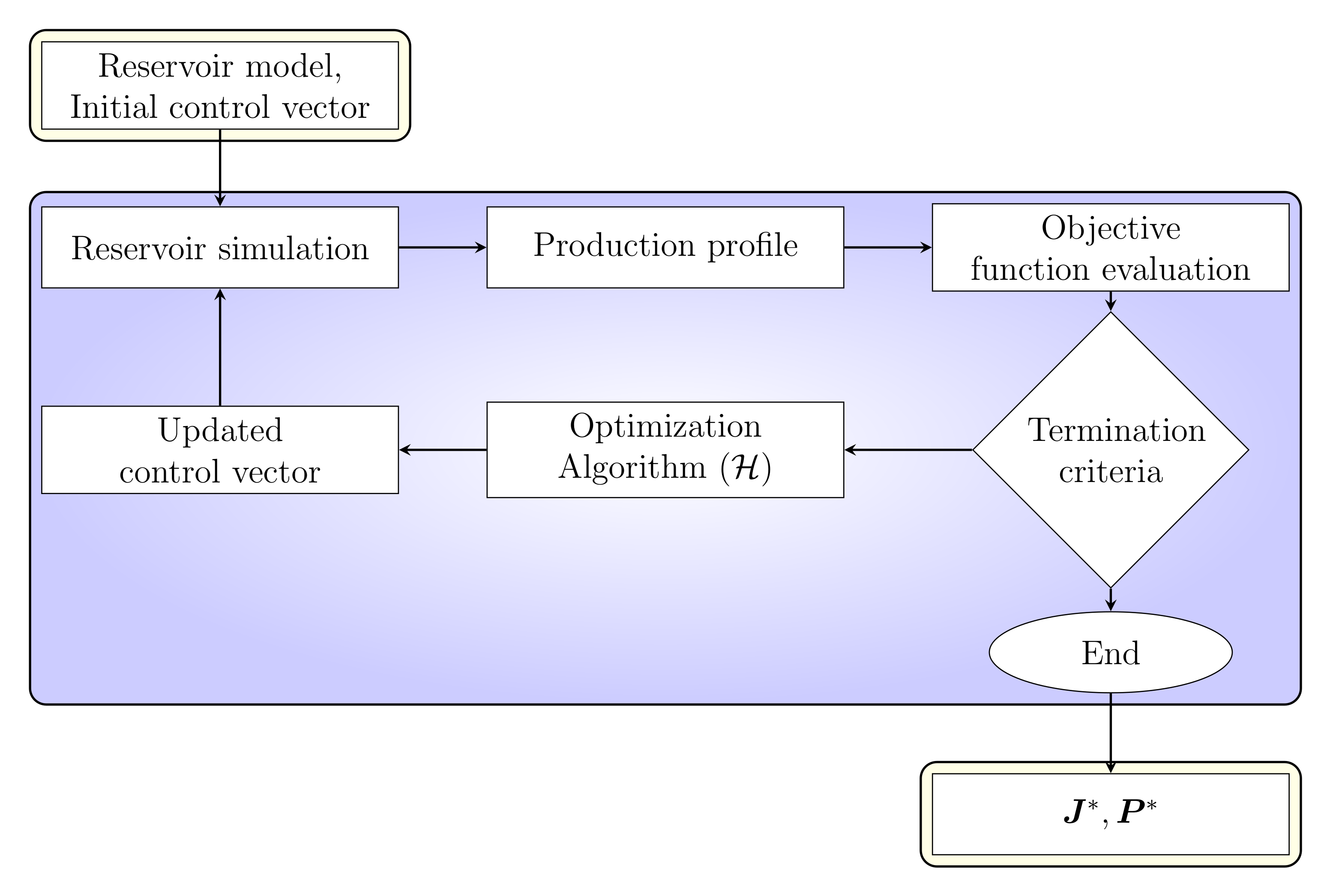
2.2.2. Optimization Algorithm

The optimization algorithm used for multilateral well placement optimization contains several modules, which allow easily enhancing its capability. The algorithm runs in a closed-loop iteration, as presented in Figure 12.

As the inputs for the optimization loop, the reservoir model and initial control vector (sets of end-points) are required. In the simulation module, the control vector is translated into simulator keywords and called the external simulator (in this case, we used Schlumberger Eclipse software). The completed simulation returns the production profile including oil, gas, and water production, as well water and gas injection if present for each well in the simulation in the given time domain. The production profile is pushed into the objective function evaluation module where project NPV is determined. The project value (NPV) is passed through the termination criterion (the difference between the iteration or a total number of iterations); if the criterion is not fulfilled, the optimization core algorithm is called. The optimization core ($\mathcal{H}$) involves control vector ${\mathit{U}}^m$ and the objective function value for that control vector $J\left({\mathit{U}}^m\right)$. In this paper, we introduce GA and PSO as the optimization core algorithm. Thus, updates to the solution of the control vector can be expressed as ${\mathit{U}}^{m+1}=\mathcal{H}\left({\mathit{U}}^m,J\left({\mathit{P}}^m\right)\right)$. The optimization algorithms used in this work are used for a certain set of solutions, called the population—$\overline{\mathit{u}}$. The population is a set consisting of H solution individuals:

$$\overline{\mathit{u}}={\{{\mathit{U}}_1,{\mathit{U}}_2,\dots ,{\mathit{U}}_H\}}^T$$

(14)

To illustrate the population, assume that the population consists of $H=5$ individual solutions. In the generation of m (the iteration of the optimization algorithm), individual solutions ${\mathit{U}}_h,h=1\dots ,H$ are located in the solution space. Each individual solution represents a certain vector of decision variables. The assessment of the population is based on the value of the objective function $J\left({\mathit{U}}_h\right),h=1\dots ,H$ for each vector of decision variables. Then, as a result of the optimization algorithm, a new population of solutions is generated: ${\mathit{U}}^{m+1}=\mathcal{H}\left({\mathit{U}}^m,J\left({\mathit{P}}^m\right)\right)$. As a result of the optimization algorithm, a population is created in which there is at least one solution satisfying the relationship: $(\exists {\mathit{U}}_h,h\in H)(J\left({\mathit{U}}_h^{m+1}\right)\ge J\left({\mathit{U}}_h^m\right))$.

3. Case Study

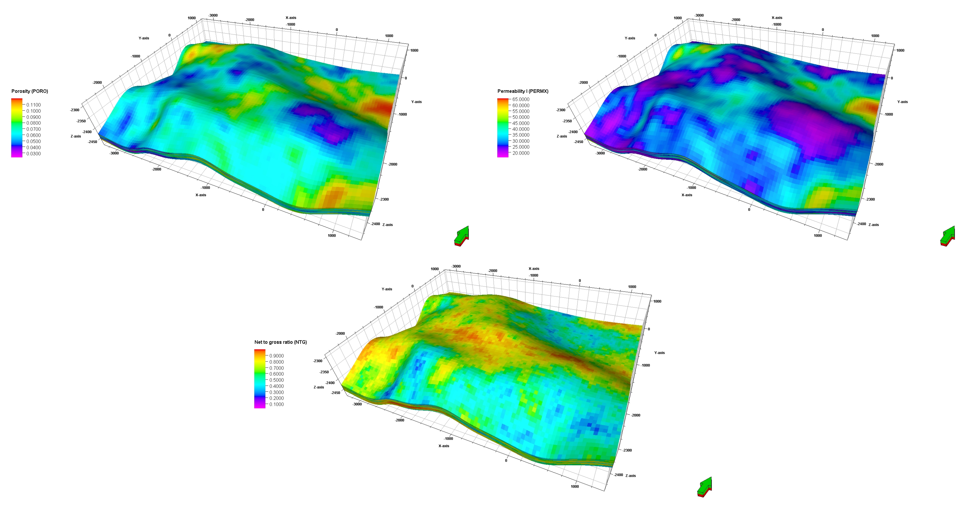
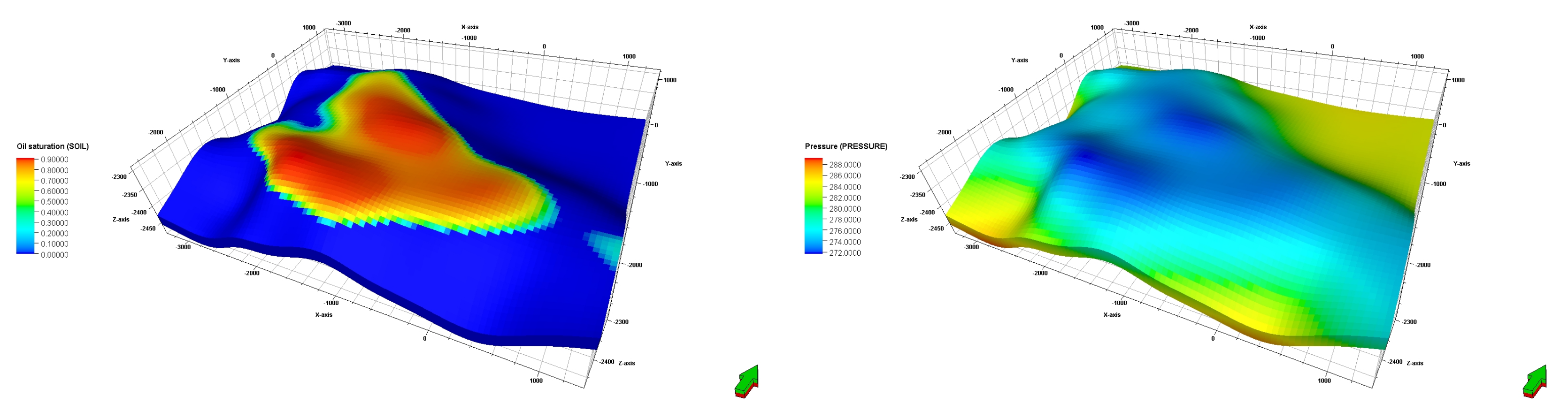
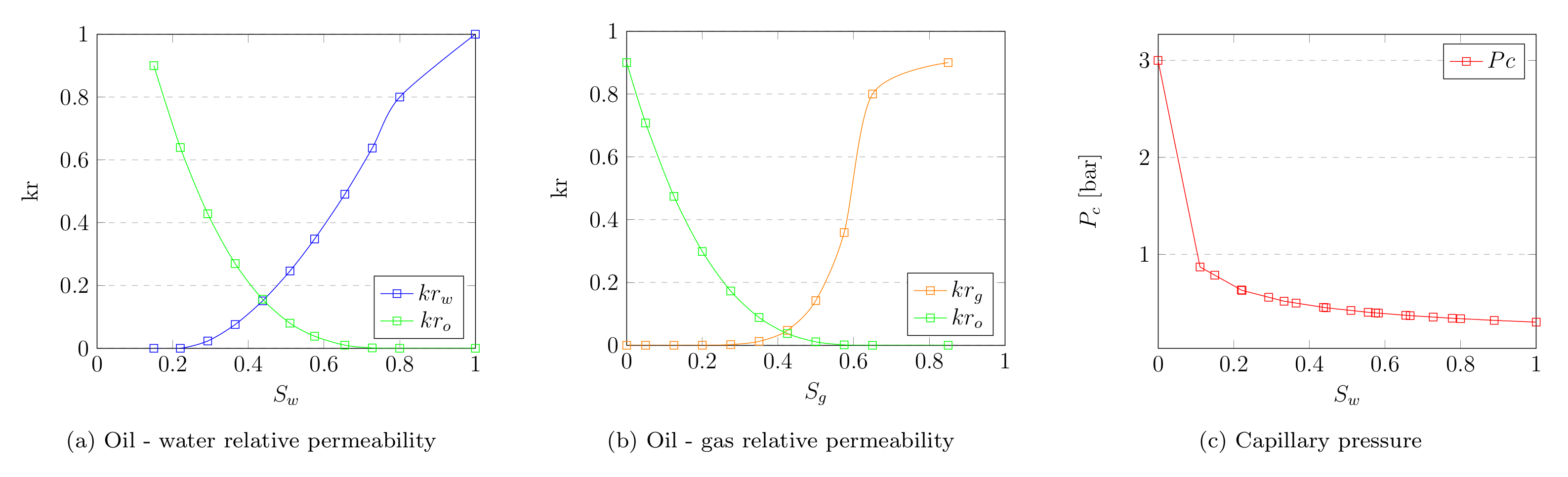
3.1. Reservoir Simulation Model

The synthetic reservoir model used in this study is a three-dimensional system and consists of a 94 × 75 × 10 grid cell arrangement ($N_x$, $N_y$, $N_z$) corresponding to the x, y, z directions, covering an area of 17.625 km${}^2$. The individual cell size is 50 × 50 × 3 m. The spatial distributions of porosity, permeability, NTG (net to gross), oil saturation, and pressure are presented in Figure 13 and Figure 14. The statistical analysis of the petrophysical properties is presented in

Table 1. Statistical analysis of the basic petrophysical parameters in the evaluated reservoir. Source: typical values for reservoirs located in the Carpathian area of Poland, internal AGH UST Drilling, Oil and Gas faculty report. Adapted from Janiga et al. [33].

	Unit	Mean	Min	Med	Max
Permeability	mD	29.205	15.800	27.070	65.456
Porosity	(-)	0.06	0.022	0.062	0.119
Net to gross	(-)	0.696	0.025	0.713	0.999
Oil saturation	(-)	0.127	0	0	0.909
Pressure	(bar)	278.833	271.690	277.967	289.096

. Fluid-rock interaction is illustrated in Figure 15.

3.2. Optimization Assumptions

Referring to the objective function of the optimization case study, several assumptions were made. The optimization time was 20 years, with a 0.5 year simulation time step. The economic parameters used for the optimization are listed in

Table 2. Economic assumptions for the optimization framework. MLW, multilateral well.

Parameter	Symbol	Unit	Value
Oil price	$r_o$	$/m${}^3$	517.94
Gas price	$r_g$	$/m${}^3$	0.03
Oil production cost	${\mathcal{S}}_o$	$/m${}^3$	103
Gas production cost	${\mathcal{S}}_g$	$/m${}^3$	0.01
Water production cost	${\mathcal{S}}_{wp}$	$/m${}^3$	8.82
Well maintenance	$K_p$	$/year	150,000
Yearly interest rate	b	%	19
Trunk drilling cost	${\mathcal{S}}_v$	$	5,900,000
MLW coefficient	$a_{MLW}$	$\$/m$	1
	$b_{MLW}$	−	2
	$c_{MLW}$	$	30,000

. The implementation of a multilateral well in reservoir management requires a high capital cost. The cost of drilling the vertical well part was taken as the average in Poland case in the Carpathian area, taking into account the reservoir depth. Branches’ drilling cost was adopted from previous field experience due to the lack of Polish MLW applications [34,35]. Hydrocarbon revenue values have a higher value, which ensures meeting the threshold of new technology in the research and development application.

The proposed end-point multilateral well algorithm was implemented in a dynamic simulation model. Each of the individual side wells provides a second layer in the numerical model ($s^{\left(z\right)}=2$). Multilateral wells are controlled by a bottom pressure of 100 bar with a limit of maximum oil production of a 25 m${}^3$/d per individual side well depending on the number of side wells. The determined BHP (bottom hole pressure) in the production well forced a single-phase flow in a reservoir (the bubble point pressure is equal to 90 bar). The optimization focused on finding discrete values for the location of end-point wells on the numerical grid represented by block coordinates (${\mathit{s}}^{\left(\mathit{x}\right)},{\mathit{s}}^{\left(\mathit{y}\right)}$) that maximize the objective function, assuming economic and technological constraints. Optimization was performed using a genetic algorithm and a particle swarm algorithm. In addition, it was assumed that the algorithms used (GA and PSO) operated on populations of $\mathit{H}=\mathbf{10}$ individuals, which means that during one iteration of the optimization algorithm (generation), 10 numerical simulations of the hydrocarbon reservoir work were performed in accordance with a given vector of decision variables. The termination condition assumed $\mathit{M}=\mathbf{50}$ iterations of the algorithm’s main loop.

The optimization was carried out for the following number of nodal points:

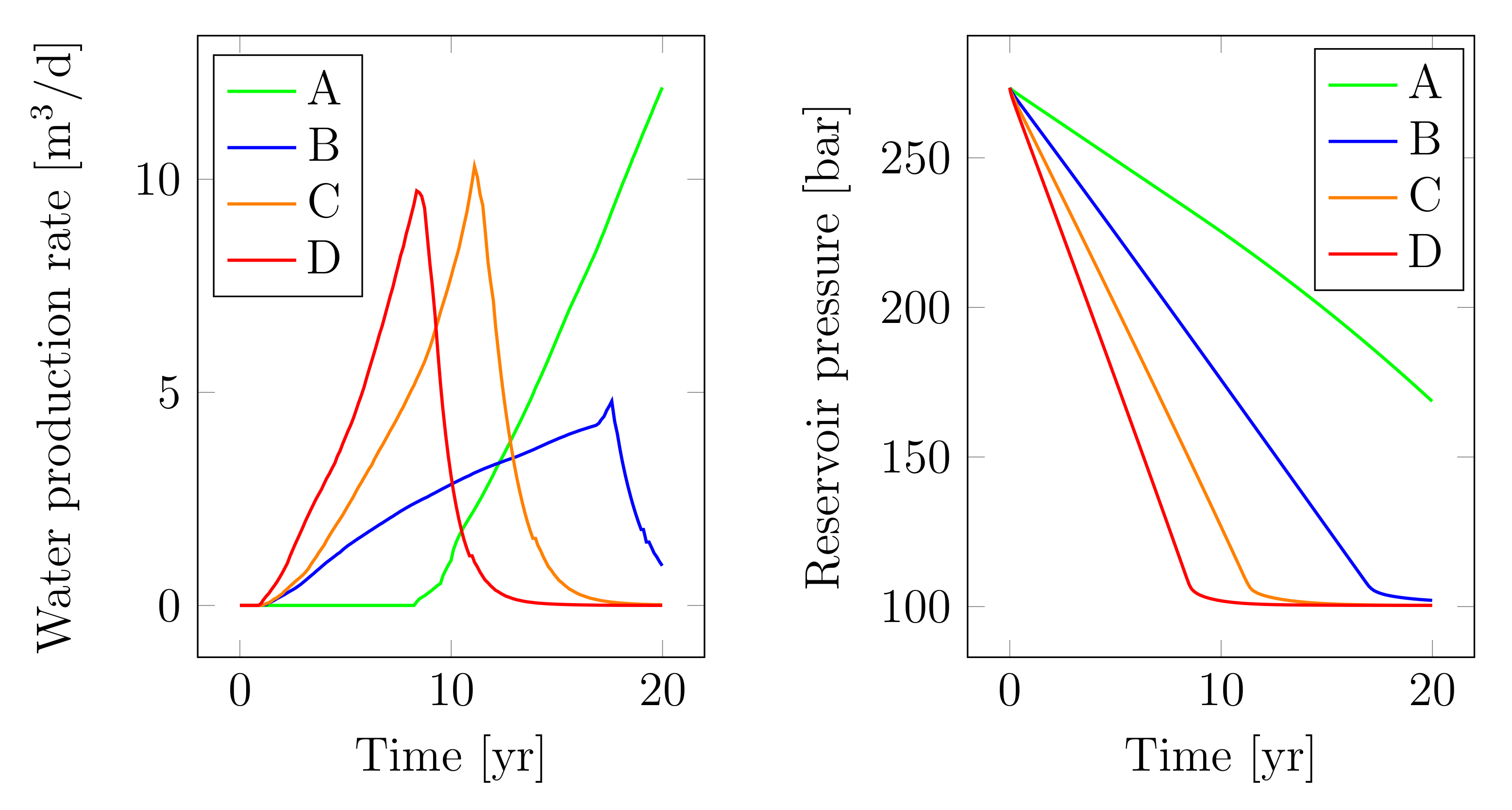
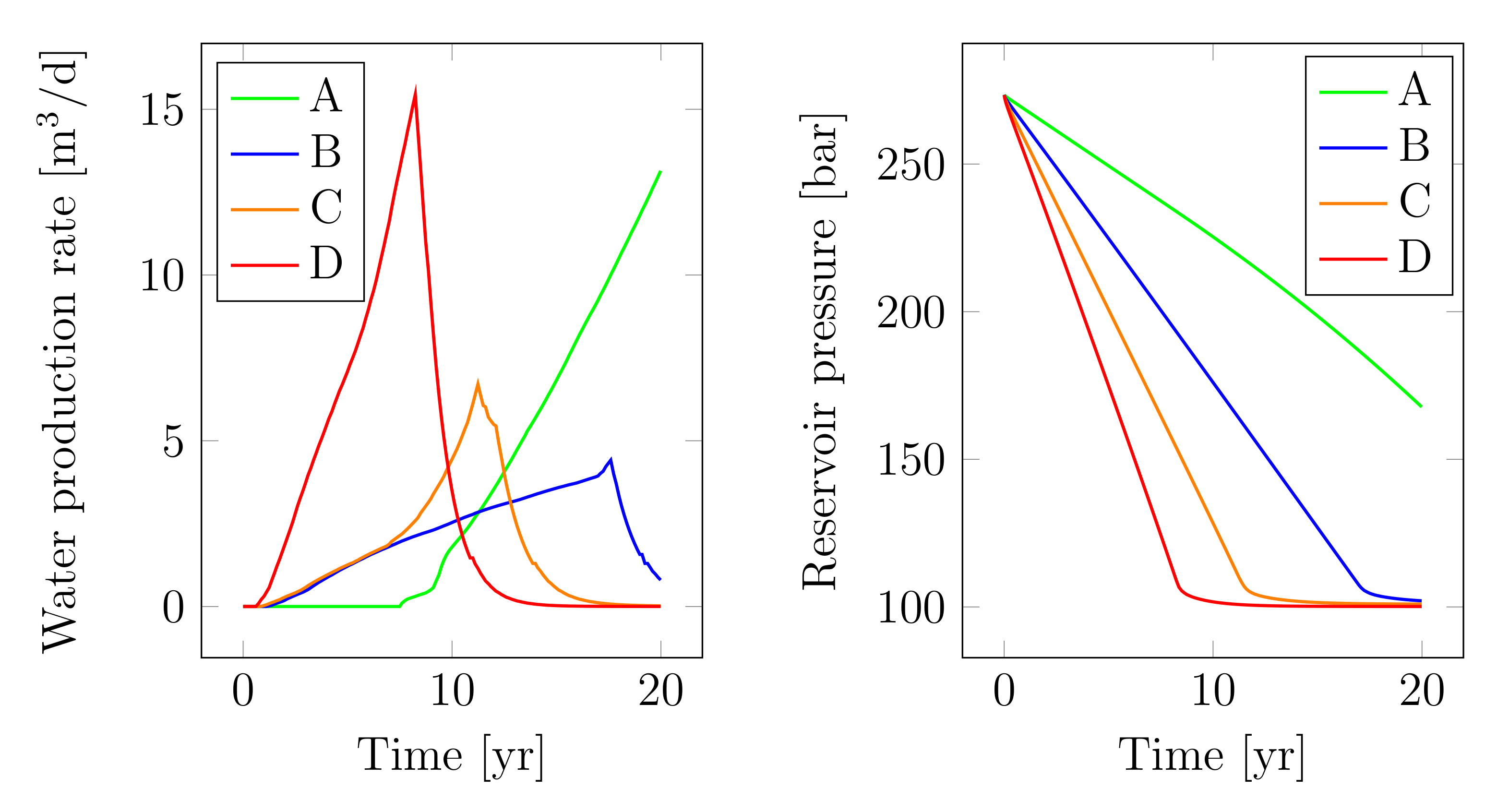
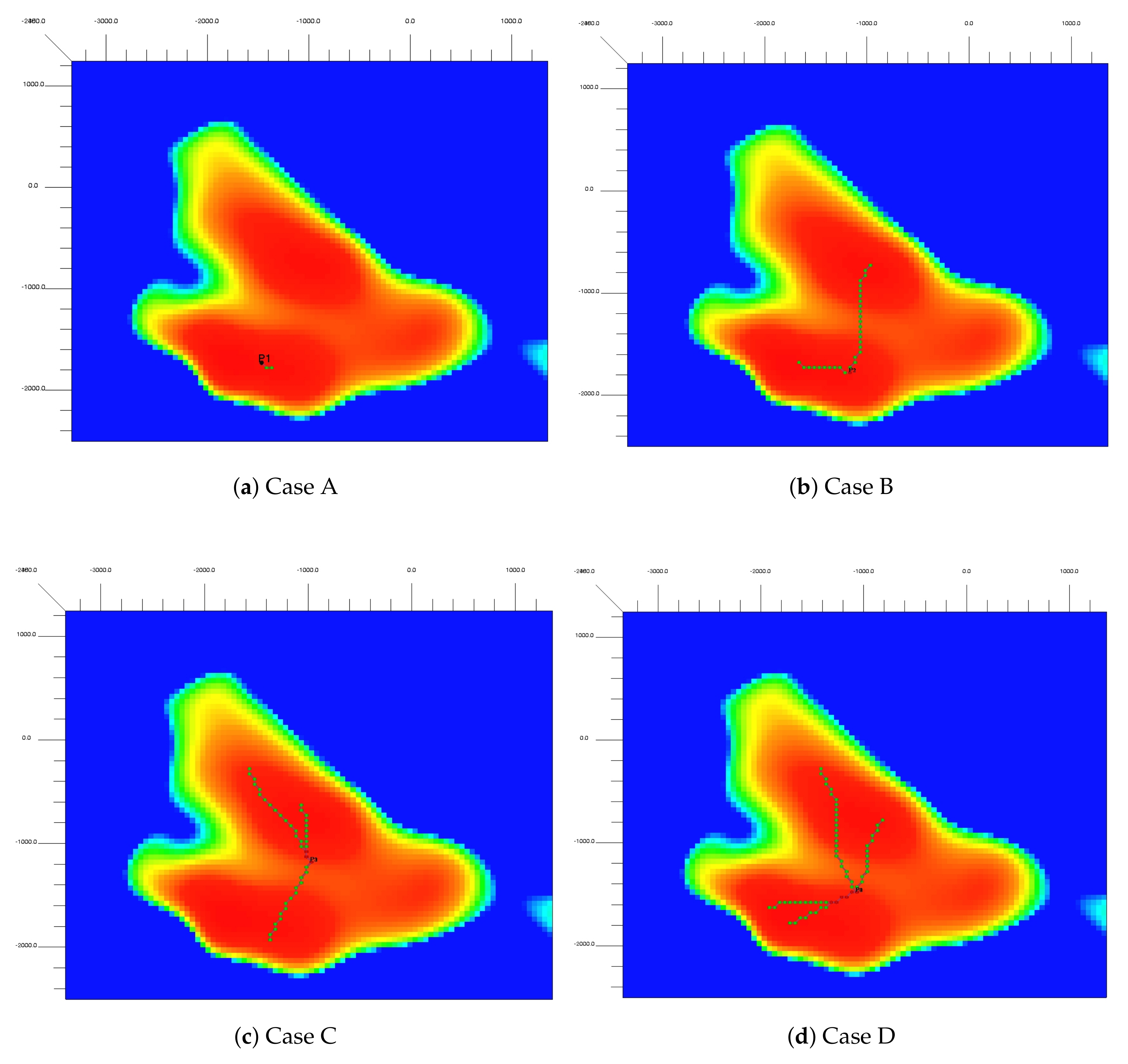
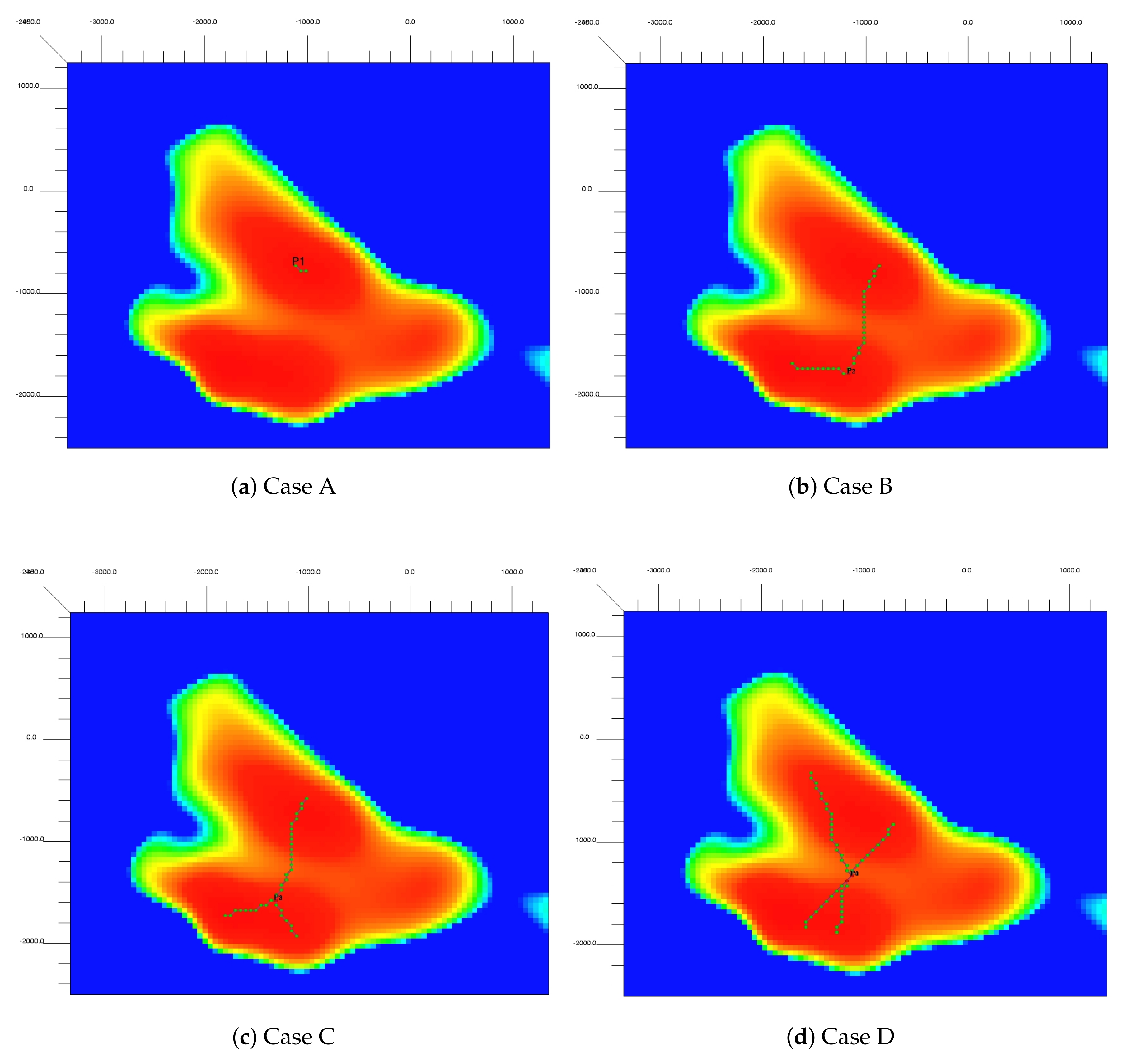
• Case A: horizontal well—$N_g$ = 2 nodal points,
• Case B: bilateral well—$N_g$ = 3 nodal points,
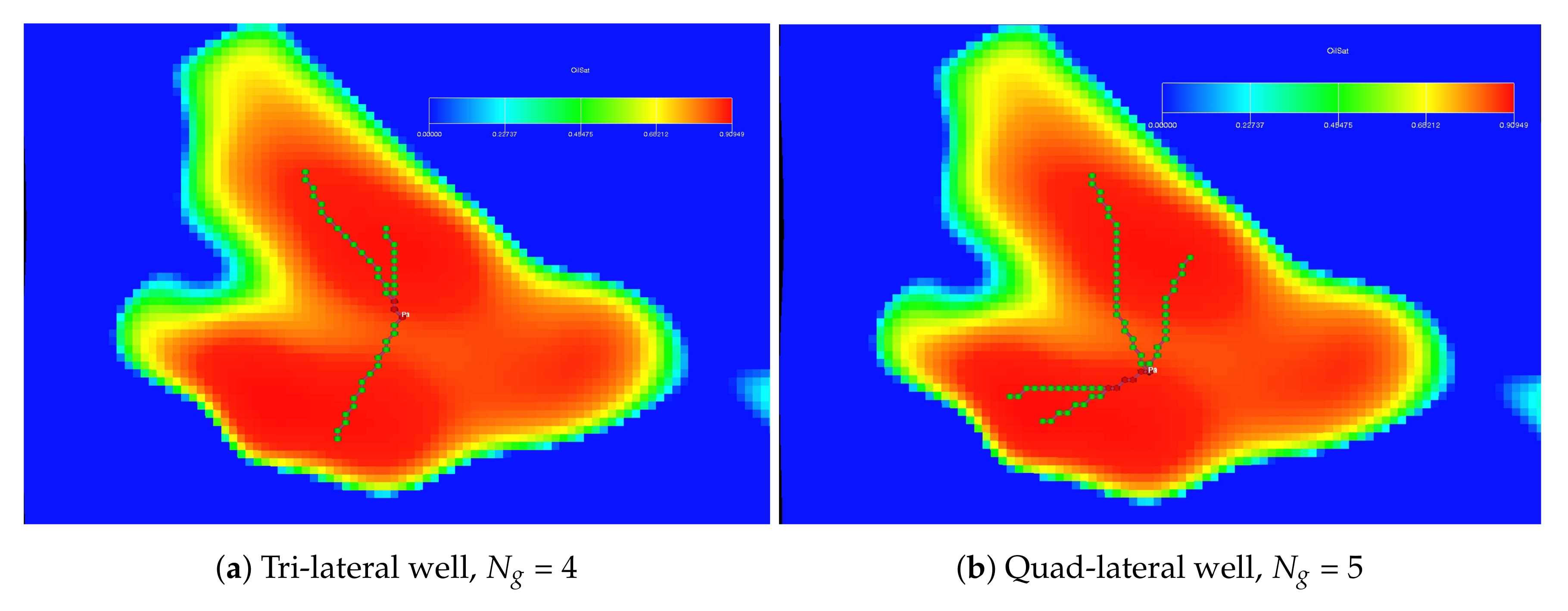
• Case C: trilateral well—$N_g$ = 4 nodal points,
• Case D: quad-lateral well—$N_g$ = 5 nodal points.

4. Results and Discussion

According to the workflow procedure and example implementation schemas, the obtained results were gathered and post-processed. Optimization runs were examined in terms of convergence and termination criteria. The reservoir performance for well design patterns was investigated, and a general cause-effect observation was made.

4.1. Reservoir Production Performance and Optimization Results

Firstly, the effect of reservoir performance on the objective function trends will be evaluated. According to Figure 16 and Figure 17, a horizontal well maintains the oil production rate control during the whole production period. With the individual control of each side well, it is possible to maintain the production at a constant level for a period of eight to 20 years with the assumed case study. The horizontal well works with constant performance throughout the entire period, regardless of the optimization algorithm chosen. The bilateral well can operate at a constant production rate for over nine years apart from the optimization algorithm. Tri- and quad-lateral wells, due to the high production rate, can operate 12.1 and 9.8 years respectively. Decreasing the hydrocarbon production rate affects the reservoir pressure and reservoir water production rate. The horizontal well pattern has the advantage of delaying reservoir water breakthrough. Reservoir brine is produced from the 10th year of the simulation time. Other well design schema have accelerated water production. The major difference between the GA and PSO optimization run is visible for the water production in Case C and is related to the modification of one well branch trajectory in a reservoir. In terms of total oil production, Cases C and D have similar end values. However, Case D promotes faster oil production, which has a significant impact on project NPV. It can be seen that increasing the number of side wells (from three to four) for both the genetic algorithm and the swarm algorithm does not increase production, but only its acceleration over time. The values of the objective function for selected locations of the end-point node are presented in

Table 3. The value of the objective function depending on the considered case; optimization of the location of multilateral wells.

Objective Function Value ($\times {10}^6\mathit{\$}$)
Variant	GA	PSO
A	61.644	61.628
B	138.183	138.175
C	179.539	181.774
D	202.976	206.480

.

The genetic algorithm and particle swarm optimization algorithm implement mechanisms to avoid local attraction areas in the objective function; however due to the stochastic realization and population upgrade mechanism, a difference between the algorithms can be noticed. Case B has minor divergence in the GA and PSO realization, but even a small well pattern design can affect the objective function. It also should be noted that for the quad-lateral well, capital expenditure is the highest; nevertheless, the acceleration of oil production affects the project NPV, indicating that type of well as the most promising to implement in the reservoir. The best results were obtained by implement the PSO algorithm for Case D, outperforming the GA run by 3.5 mln $. A major concern in Case D is the relatively high reservoir water production from the beginning of production. The end-point well location can affect the reservoir’s performance and project profitability.

4.2. Results of Multilateral Well Placement in the 3D Spatial Domain

The optimal solutions for the location of the nodal points of the multilateral wells obtained using optimization algorithms are presented in

Table 4. Coordinate of the block $s^{\left(x\right)},s^{\left(y\right)}$ enclosed end-point set for the multilateral well, GA algorithm.

Nodal Points ${\mathit{s}}^{\left(\mathit{x}\right)},{\mathit{s}}^{\left(\mathit{y}\right)}$
Case	Center Point $\breve{\mathit{P}}$	End-Points $\mathit{P}$
A	(38,60)	(40,61)
B	(44,61)	(34,59)(48,40)
C	(46,38)	(36,31)(40,64)(48,49)
D	(46,55)	(51,41)(39,31)(29,58)(33,61)

and

Table 5. Coordinate of the block $s^{\left(x\right)},s^{\left(y\right)}$ enclosed end-point set for multilateral well, PSO algorithm.

Nodal Points ${\mathit{s}}^{\left(\mathit{x}\right)},{\mathit{s}}^{\left(\mathit{y}\right)}$
Case	Center Point $\breve{\mathit{P}}$	End-Points $\mathit{P}$
A	(45,40)	(47,41)
B	(44,61)	(33,59)(50,40)
C	(44,57)	(47,37)(31,30)(45,64)
D	(45,49)	(37,32)(36,63)(42,63)(55,42)

.

Small changes of the end-point positions can change the project profitability, increase the water production rate, accelerate water breakthrough, and increase the utilization of reservoir energy. The result of the optimization algorithm, multilateral trajectories, was implemented on a numerical grid, which is presented in Figure 18 and Figure 19. The objective function for wells with a complex trajectory takes into account their length; therefore, the results obtained should be treated as optimal in terms of location and length. A list of the lengths of individual well branches is shown in

Table 6. Multilateral well length including individual branches.

Case	Distance between Points (m)				Total (m)
GA algorithm
A	111.8				111.8
B	509.9	1068.88			1578.78
C	559.02	850	1081.67		2490.69
D	715.89	743.3	863.13	1250	3572.32
PSO algorithm
A	111.8				111.8
B	559.02	1092.02			1651.04
C	403.11	522.02	1044.03		1969.16
D	570.09	640.31	672.68	1077.03	2960.11

. Considering the total well length, GA and PSO propose the same length for Case A. PSO promotes a shorter total well length pattern, which can be addressed as drilling risk mitigation.

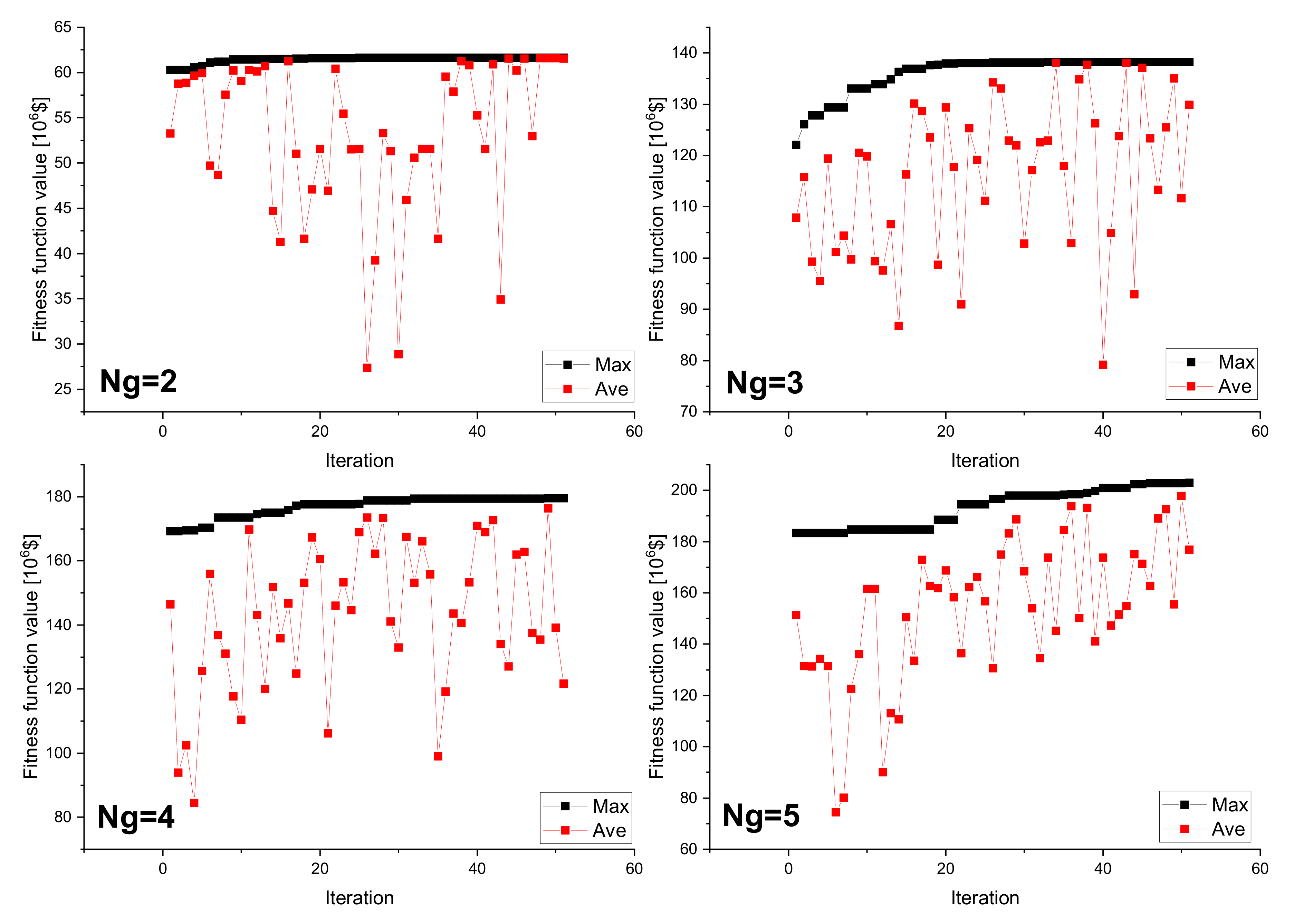
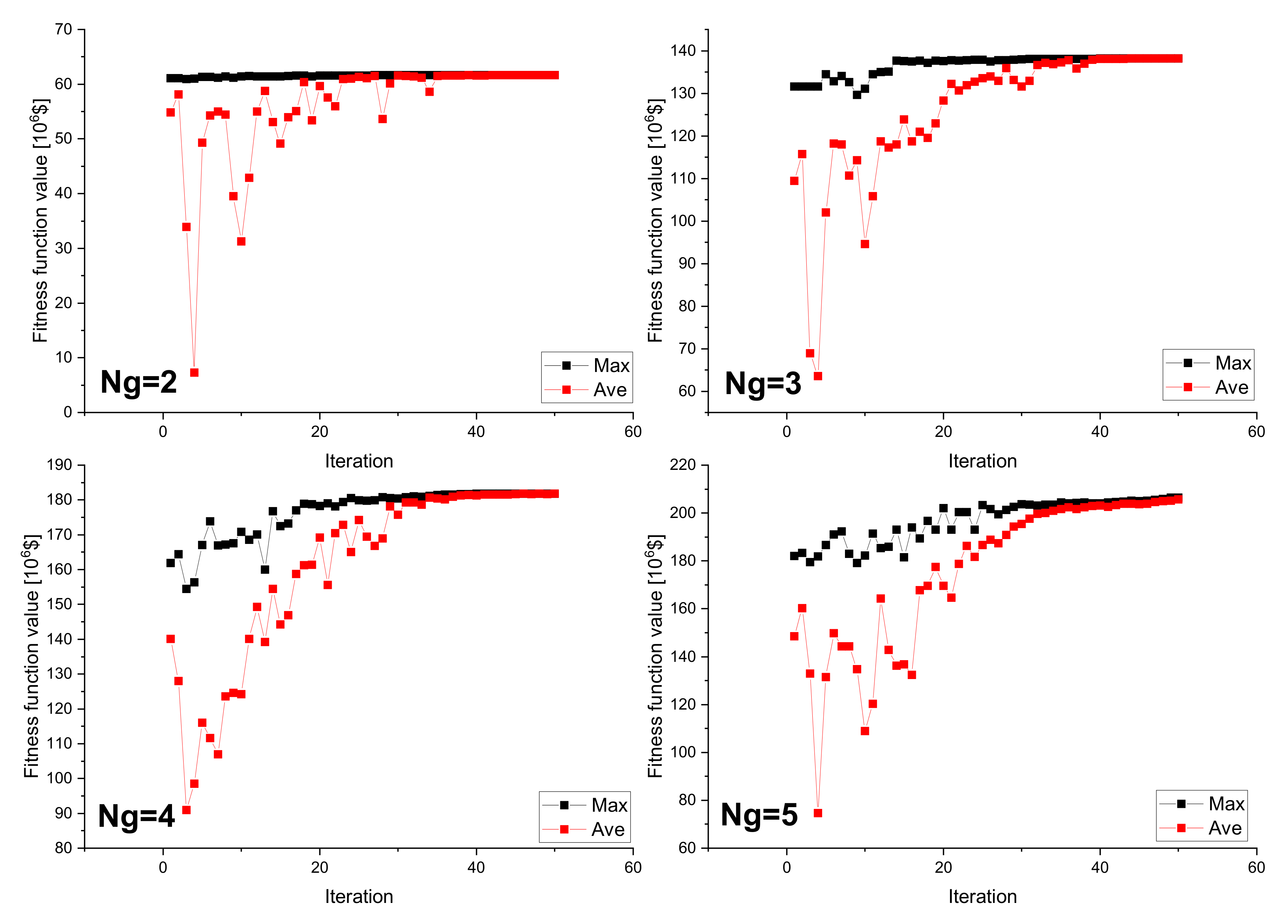
4.3. Optimization Run Convergence

Changes in the average and best population fit for the considered case study of implementation of the multi-bottom well are shown in Figure 20 and Figure 21. For both the genetic algorithm and the particle swarm algorithm, a monotonic increase in the maximum values of the target function was observed during the algorithm operation. The optimization run for each of the multilateral well patterns was terminated in the case of exceeding the number of iterations or the flattening of objection function trends. In all of the cases, the optimization was terminated by the number of iterations. The genetic algorithm has a slower convergence ratio, especially for complex problems (Cases C and D). This is related to the number of decision variables; enhancing the problem search space simultaneously required several iterations to meet the convergence criteria. Both GA and PSO implement a fine-tuning mechanism; however, that part was not evaluated on this paper.

4.4. Model Limitation

The proposed model is currently under further improvement; thus, some limitations of application can be listed. The current end-point model development required extensive testing with various reservoir grid sizes and numbers of cells. However, all tests were performed on orthogonal cell distributions along with the numerical model. That assumption is fulfilled by the Schlumberger Petrel (Version: 2019, Manufacturer: Schlumberger) software used in this study, which develops a reservoir numerical model from geological model forcing cell orthogonality. The impact of cell geometry on the multilateral well trajectory is meaningless, due to the fact that the model evaluates true spatial coordinates. Our preliminary investigation shows that the end-point model can be effectively implemented in any numerical model as long as a multilateral well is placed in a global grid or a local grid directly. The mixing of global and local grid placement is currently forbidden. It also should be noted that the increase of the total cell number in the reservoir model can significantly increase the solution search space, which may lead to optimization conversion failure. We recommended performing a coarse optimization run to establish a promising search space and reduce the search space in the case of fine grid optimization.

5. Conclusions

The assumed goal of the work was achieved, and based on the results obtained, the following conclusions can be made:

• It seems necessary to use a minimum of two different optimization methods to validate the quality of the solutions obtained,
• The optimization model developed can be used to complement the manual search method,
• Multilateral wells will be concerned as a must in the effective management of hydrocarbon reservoirs, especially in an off-shore application; thus, optimization of trajectory planning should be taken into consideration,
• The proposed end-point optimization model integrates well trajectory planning with the reservoir model; thus, the obtained results can be used in effective reservoir management in different time domains,
• Our end-point algorithm is easily implemented in the reservoir model and, based on the application of the population-type optimization algorithm, is time-efficient, as well as effortlessly scalable among various models.

References

- Janiga, D. Model Optymalizacji Udostepnienia i Eksploatacji Zloza Weglowodorow z Wykorzystaniem Sztucznej Inteligencji. Ph.D. Thesis, AGH University of Science and Technology, Krakow, Poland, 2017. [Google Scholar]
- Yue, P.; Jia, B.; Sheng, J.; Lei, T.; Tang, C. A coupling model of water breakthrough time for a multilateral horizontal well in a bottom water-drive reservoir. J. Pet. Sci. Eng. 2019, 177, 317–330. [Google Scholar] [CrossRef]
- Stopa, J.; Rychlicki, S.; Wojnarowski, P.; Kosowski, P. Zastosowanie odwiertow rozgalezionych w eksploatacji zloz ropy i gazu. Wiertnictwo Naft. Gaz 2007, 24, 869–876. [Google Scholar]
- Elyasi, S. Assessment and evaluation of degree of multilateral well’s performance for determination of their role in oil recovery at a fractured reservoir in Iran. Egypt. J. Pet. 2016, 25, 1–14. [Google Scholar] [CrossRef][Green Version]
- Chin, W.C. Quantitative Methods in Reservoir Engineering; Gulf Professional Publishing: Houston, TX, USA, 2002. [Google Scholar]
- Tangparitkul, S. Evaluation of effecting factors on oil recovery using the desirability function. J. Pet. Explor. Prod. Technol. 2018, 8, 1199–1208. [Google Scholar] [CrossRef]
- Abusahmin, B.S.; Karri, R.R.; Maini, B.B. Influence of fluid and operating parameters on the recovery factors and gas oil ratio in high viscous reservoirs under foamy solution gas drive. Fuel 2017, 197, 497–517. [Google Scholar] [CrossRef]
- Song, X.; Zhang, C.; Shi, Y.; Li, G. Production performance of oil shale in-situ conversion with multilateral wells. Energy 2019, 189, 116145. [Google Scholar] [CrossRef]
- Wei, Y.; Jia, A.; Wang, J.; Luo, C.; Qi, Y. Semi-analytical Modeling of Pressure-Transient Response of Multilateral Horizontal Well with Pressure Drop along Wellbore. J. Nat. Gas Sci. Eng. 2020, 80, 103374. [Google Scholar] [CrossRef]
- Yang, Y.; Cui, S.; Ni, Y.; Zhang, G.; Li, L.; Meng, Z. Key technology for treating slack coal blockage in CBM recovery: A case study from multi-lateral horizontal wells in the Qinshui Basin. Nat. Gas Ind. B 2016, 3, 66–70. [Google Scholar] [CrossRef][Green Version]
- Chen, D.; Pan, Z.; Liu, J.; Connell, L.D. Characteristic of anisotropic coal permeability and its impact on optimal design of multi-lateral well for coalbed methane production. J. Pet. Sci. Eng. 2012, 88, 13–28. [Google Scholar] [CrossRef]
- Zhou, S.W.; Sun, F.J.; Zeng, X.L.; Fang, M.J. Application of multilateral wells with limited sand production to heavy oil reservoirs. Pet. Explor. Dev. 2008, 35, 630–635. [Google Scholar] [CrossRef]
- Shi, Y.; Song, X.; Wang, G.; McLennan, J.; Forbes, B.; Li, X.; Li, J. Study on wellbore fluid flow and heat transfer of a multilateral-well CO2 enhanced geothermal system. Appl. Energy 2019, 249, 14–27. [Google Scholar] [CrossRef]
- Aadnøy, B.S. Technology Focus: Multilateral and Complex-Trajectory Wells. J. Pet. Technol. 2019, 71, 71. [Google Scholar] [CrossRef]
- Lyu, Z.; Song, X.; Li, G. A semi-analytical method for the multilateral well design in different reservoirs based on the drainage area. J. Pet. Sci. Eng. 2018, 170, 582–591. [Google Scholar] [CrossRef]
- Lyu, Z.; Song, X.; Geng, L.; Li, G. Optimization of multilateral well configuration in fractured reservoirs. J. Pet. Sci. Eng. 2019, 172, 1153–1164. [Google Scholar] [CrossRef]
- Buhulaigah, A.; Al-Mashhad, A.S.; Al-Arifi, S.A.; Al-Kadem, M.S.; Al-Dabbous, M.S. Multilateral wells evaluation utilizing artificial intelligence. In Proceedings of the SPE Middle East Oil & Gas Show and Conference, Manama, Bahrain, 6–9 March 2017; Society of Petroleum Engineers: Richardson, TX, USA, 2017. Available online: https://www.onepetro.org/conference-paper/SPE-183688-MS (accessed on 15 June 2020).
- Garrouch, A.A.; Lababidi, H.M.; Ebrahim, A.S. A web-based expert system for the planning and completion of multilateral wells. J. Pet. Sci. Eng. 2005, 49, 162–181. [Google Scholar] [CrossRef]
- Xu, B.; Baird, R.; Vukovich, G. Fuzzy evolutionary algorithms and automatic robot trajectory generation. In Methods and Applications of Intelligent Control; Springer: Dordrecht, The Netherlands, 1997; pp. 423–449. [Google Scholar]
- Miller, B.L.; Goldberg, D.E. Genetic algorithms, tournament selection, and the effects of noise. Complex Syst. 1995, 9, 193–212. [Google Scholar]
- Alajmi, A.; Wright, J. Selecting the most efficient genetic algorithm sets in solving unconstrained building optimization problem. Int. J. Sustain. Built Environ. 2014, 3, 18–26. [Google Scholar] [CrossRef]
- Eberhart, C.; Kennedy, J. A new optimizer using particle swarm theory. In Proceedings of the Sixth International Symposium on Micro Machine and Human Science, Nagoya, Japan, 4–6 October 1995; IEEE: New York, NY, USA, 1995; Volume 1, pp. 39–43. [Google Scholar]
- Kennedy, J. Particle swarm optimization. In Encyclopedia of Machine Learning; Springer: Berlin/Heidelberg, Germany, 2011; pp. 760–766. [Google Scholar]
- Shi, Y.; Eberhart, R. A modified particle swarm optimizer. In Proceedings of the 1998 IEEE International Conference on Evolutionary Computation Proceedings. IEEE World Congress on Computational Intelligence (Cat. No.98TH8360), Anchorage, AK, USA, 4–9 May 1998; pp. 69–73. [Google Scholar]
- Almeida, L.F.; Tupac, Y.J.; Pacheco, M.A.C.; Vellasco, M.M.B.R.; Lazo, J.G.L. Evolutionary optimization of smart-wells control under technical uncertainties. In Proceedings of the Latin American & Caribbean Petroleum Engineering Conference, Buenos Aires, Argentina, 15–18 April 2007; Society of Petroleum Engineers: Richardson, TX, USA, 2007. Available online: https://www.onepetro.org/conference-paper/SPE-107872-MS (accessed on 15 June 2020).
- Awotunde, A.A.; Sibaweihi, N. Consideration of voidage-replacement ratio in well-placement optimization. SPE Econ. Manag. 2014, 6, 40–54. [Google Scholar] [CrossRef]
- Bellout, M.C.; Echeverría Ciaurri, D.; Durlofsky, L.; Foss, B.; Kleppe, J. Joint optimization of oil well placement and controls. Comput. Geosci. 2012, 16, 1061–1079. [Google Scholar] [CrossRef]
- Brouwer, D.; Jansen, J. Dynamic Optimization of Waterflooding With Smart Wells Using Optimal Control Theory. In Proceedings of the European Petroleum Conference, Aberdeen, UK, 29–31 October 2002. [Google Scholar] [CrossRef]
- Doublet, D.C.; Aanonsen, S.I.; Tai, X.C. An efficient method for smart well production optimisation. J. Pet. Sci. Eng. 2009, 69, 25–39. [Google Scholar] [CrossRef]
- Forouzanfar, F.; Reynolds, A. Well-placement optimization using a derivative-free method. J. Pet. Sci. Eng. 2013, 109, 96–116. [Google Scholar] [CrossRef]
- Gross, H. Response surface approaches for large decision trees: Decision making under uncertainty. In Proceedings of the ECMOR XIII-13th European Conference on the Mathematics of Oil Recovery, Biarritz, France, 10–13 September 2012. [Google Scholar]
- Isebor, O.J.; Durlofsky, L.J. Biobjective optimization for general oil field development. J. Pet. Sci. Eng. 2014, 119, 123–138. [Google Scholar] [CrossRef]
- Janiga, D.; Czarnota, R.; Stopa, J.; Wojnarowski, P. Self-adapt reservoir clusterization method to enhance robustness of well placement optimization. J. Pet. Sci. Eng. 2019, 173, 37–52. [Google Scholar] [CrossRef]
- El-Sayed, A.A.H.; AI-Awad, M.; Al-Blehed, M.; Al-Saddiqui, M. An Economic Model for Assessing the Feasibility of Multilateral Wells. J. King Saud Univ.-Eng. Sci. 2001, 13, 153–176. [Google Scholar] [CrossRef]
- Manshad, A.K.; Dastgerdi, M.E.; Ali, J.A.; Mafakheri, N.; Keshavarz, A.; Iglauer, S.; Mohammadi, A.H. Economic and productivity evaluation of different horizontal drilling scenarios: Middle East oil fields as case study. J. Pet. Explor. Prod. Technol. 2019, 9, 2449–2460. [Google Scholar] [CrossRef]